Sensitivity of the Cosmic Microwave Background Anisotropy to Initial Conditions in Quintessence Cosmology

Abstract

We analyze the evolution of energy density fluctuations in cosmological scenarios with a mixture of cold dark matter and quintessence, in which the quintessence field is modeled by a constant equation of state. We obtain analytic expressions for the time evolution of the quintessence perturbations in models with light fields. The fluctuations behave analogously to a driven harmonic oscillator, where the driving term arises from the inhomogeneities in the surrounding cosmological fluid. We demonstrate that the homogeneous solution, determined by the initial conditions, is completely sub-dominant to the inhomogeneous solution for physically realistic scenarios. Thus we show that the cosmic microwave background anisotropy predicted for such models is highly insensitive to the initial conditions in the quintessence field.

1 Introduction

Growing observational evidence suggests that the total matter density of the universe is significantly less than the critical density. Yet, measurements of the cosmic microwave background (CMB) indicate that the universe is flat and the total energy density is precisely equal to the critical density [1]. Candidates for the missing energy are the cosmological constant ($\Lambda$) [2], and quintessence ($Q$), a time-varying, spatially inhomogeneous component with negative pressure [3, 4]. Examples of quintessence include slowly evolving fields or topological defects such as a network of light and tangled cosmic strings [8]-[14]. Cold Dark Matter (CDM) models with quintessence ($Q$CDM) which fit the data from observations of high red shift supernovas, gravitational lensing, CMB anisotropy, and structure formation [1]-[3] have been found.

For the purposes of this paper, we model quintessence as a scalar field quintessence rolling down a potential $V(Q)$ with an equation of state $w\equiv p_{Q}/\rho_{Q}$, where $p_{Q}$ is the pressure and $\rho_{Q}$ is the energy density of the field. We consider here a large class of models in which the field and fluctuation evolution may be represented by a constant equation of state with value between 0 and -1, and in which the sound speed in quintessence fluctuations, $c_{sQ}^{2}$, approaches unity at scales much smaller than the horizon. Most models of quintessence that have appeared in the literature satisfy these conditions. This class includes not only “tracker models”, which have dynamical attractor behavior, but also more general potentials [9]-[13]. We show that, in such models, the CMB anisotropy is insensitive to initial conditions of the quintessence field. By insensitive we mean that the fractional change in the CMB anisotropy power spectrum due to a change in initial conditions cannot be observationally resolved.

These conclusions were originally mentioned in our first paper on quintessence models [4], and also by others [5, 6, 7], who noted that the amplitude of the energy density perturbations in the background fluid are largely independent of the initial conditions in the scalar field, provided the initial energy contrast is less than unity. Our present work is consistent with these earlier conclusions. However, we go further in this paper by examining in detail the behavior of the scalar field perturbations, and the causes for the insensitivity, as described next.

In the next section we derive the equations of motion for the evolution of the $Q$-field and its fluctuations. We introduce a formalism to numerically study the quintessence fluctuations in terms of the evolution of the equation of state as a function of cosmological scale-factor. In section 3 we show that models with constant equation of state represent the behavior of a large class of models with light fields and monotonically evolving equations of state. In section 4 we analytically solve the fluctuation equation for constant equation of state at large wavelengths. We use this solution to describe key features of the fluctuation evolution obtained from the numerical integration. Finally, in section 5 we report the effect of changing initial conditions on quintessence fluctuation evolution and CMB anisotropy. We show that the anisotropy is highly insensitive to changes in the initial conditions.

2 Field and fluctuation equations

We consider a matter-quintessence Lagrangian of the form

$$L=L_{B}+L_{Q},$$ (1)

where the B refers to all the background species of particles and fields, including baryons, photons, cold dark matter, and neutrinos. The background cosmology is described by the Friedman-Robertson-Walker metric with positive signature. We model the $Q$-field as a classical, self-interacting, scalar field, minimally coupled to other constituents of the universe through gravity,

$$L_{Q}={1\over 2}Q_{,\mu}Q^{,\mu}-V(Q).$$ (2)

We only consider models with canonical kinetic energy terms, since $c_{sQ}^{2}$ approaches unity at scales much smaller than the horizon [4] in these models.

The time evolution of the quintessence field is determined by the equation of motion

$$Q^{\prime\prime}+2{a^{\prime}\over a}Q^{\prime}+a^{2}{\partial V\over\partial Q}=0,$$ (3)

where $a$ is the scale-factor, normalized to unity today, and where the prime (^′) represents $\partial/\partial\tau$, the derivative with respect to conformal time. By specifying the functional form of the potential, $V(Q)$, along with initial conditions $Q,\,Q^{\prime}$ at a time $\tau_{init}$, the subsequent evolution is determined for all times $\tau>\tau_{init}$.

At the scales of interest for the cosmic microwave background ($>1Mpc$), fluctuation amplitudes of the $Q$-field and the metric are usually small compared to the fields themselves, and thus a linearization of the $Q$-field and Einstein equations in the perturbation suffices to describe the fluctuation dynamics. Our analysis, carried out in the synchronous gauge, uses the conventions and equations from Ma and Bertschinger [17].

The synchronous gauge is defined by the condition that the time-time and time-space part of the metric are not perturbed. The perturbed metric is given as:

$$ds^{2}=a^{2}(\tau)\{-d\tau^{2}+(\delta_{ij}+h_{ij})dx^{i}dx^{j}\}\,.$$ (4)

The metric perturbation $h_{ij}$ can be decomposed into a trace part $h\equiv h_{ii}$ and a traceless part $\eta$. To enable us to study fluctuations as a function of wavelength, we will work in Fourier space ($\vec{k}$) with perturbations $h(\vec{k},\tau)$ and $\eta(\vec{k},\tau)$.

The time evolution of the perturbed metric is obtained by linearizing the Einstein Equations in Fourier space (see [17]). The cosmological perturbation equations for the dynamical $Q$-component are obtained by expanding the scalar field equations about the homogeneous background. In the synchronous gauge, we can write down the equation for small fluctuations $\delta Q$ in Fourier space:

$$\delta Q^{\prime\prime}+2{a^{\prime}\over a}\delta Q^{\prime}+(a^{2}{\partial^{2}V\over\partial Q^{2}}+k^{2})\delta Q=-{1\over 2}h(\vec{k},\tau)^{\prime}Q^{\prime}.$$ (5)

The fluctuation amplitude evolves in time like a scalar field.

To compute the quintessence fluctuation evolution and CMB anisotropy power spectrum, we use the fluctuation and Einstein equations to evolve the moments of the photon distribution in a Boltzmann code. We modified two separate Boltzmann codes, CMBFAST ([15]) and LINGER ([17]), by adding in scalar field evolution, and repeated all computations in the conformal gauge. The results from these multiple approaches were all identical to better than 1 part in $10^{8}$ [16].

We can parameterize quintessence models in terms of the evolution of the equation of state as a function of scale-factor $w(a)$. The formulation is useful in studying the time dependence of quintessence fluctuations and in unearthing the similarities in time evolution of models with different potentials. The energy density and pressure of the $Q$-component in this parameterization are given by

$$\rho_{Q}(a)={3H^{2}_{0}\Omega_{Q}\over 8\pi G}\exp{\Big{(}3\big{[}-\log a+\int^{1}_{a}{d\tilde{a}\over\tilde{a}}\,w(\tilde{a})\big{]}\Big{)}},$$ (6)

and

$$\qquad p_{Q}(a)=w(a)\rho_{Q}(a),$$ (7)

where $H_{0}$ is the present-day value of the Hubble constant, and $\Omega_{Q}$ is the present-day $Q$-field energy density as a fraction of the critical energy density.

To obtain the equations of motion in terms of the equation of state, we express the first and second derivative of the potential in terms of $w$:

$$a^{2}V_{,Q} = -{1\over 2}\Big{(}3{a^{\prime}\over a}(1-w)+{w^{\prime}\over 1+w}\Big{)}Q^{\prime},$$ (8)

$$a^{2}V_{,QQ} = -{3\over 2}(1-w)\Big{[}{a^{\prime\prime}\over a}-\Big{(}{a^{\prime}\over a}\Big{)}^{2}\Big{(}{7\over 2}+{3\over 2}w\Big{)}\Big{]}$$ (11)

$$+{1\over 1+w}\Big{[}{w^{\prime 2}\over 4(1+w)}-{w^{\prime\prime}\over 2}+w^{\prime}{a^{\prime}\over a}(3w+2)\Big{]}.$$

If we define $\delta\psi=\delta Q/\sqrt{1+w(\tau)}$ and $\psi^{\prime}=Q^{\prime}/\sqrt{1+w(\tau)}$, we can use Eqs. 8 and 11 to convert the field (Eq. 3) and fluctuation (Eq. 5) equations for the $Q$-field into a form in which the potential is implicit:

$$\psi^{\prime\prime}+\Big{(}(1+3w){a^{\prime}\over a}\Big{)}\frac{\psi^{\prime}}{2}=0,$$ (12)

and

$${\delta\psi^{\prime\prime}+\Big{(}2{a^{\prime}\over a}+{w^{\prime}\over 1+w}\Big{)}\delta\psi^{\prime}}$$

$$+\Big{(}k^{2}-{3\over 2}(1-w)\Big{[}{a^{\prime\prime}\over a}-\Big{(}{a^{\prime}\over a}\Big{)}^{2}\Big{(}{7\over 2}+{3\over 2}w\Big{)}\Big{]}+3w^{\prime}{a^{\prime}\over a}\Big{)}\delta\psi$$

$$=-{1\over 2}h^{\prime}\psi^{\prime}$$ (13)

A practical consequence of this change of variables is that w” drops out of the evolution equation, and we only need to specify w and w’ as functions of time. Thus, given a well sampled table of the equation of state history $w(a)$, we can numerically integrate this equation in a Boltzmann code to obtain the evolution of the quintessence field and its fluctuations.

3 Why constant $w$ approximates well a large range of potentials

For quintessence models described by a scalar field with potential $V(Q)$, the equation of state varies with the scale-factor, depending on the initial conditions on $Q$, and the form of $V(Q)$. In certain cases, especially for large mass fields (e.g. harmonic potential with large mass field, $m>>H_{0}$), the evolution is oscillatory. In most cases, however, the mass of the quintessence field is smaller than or comparable to the Hubble parameter ($m\mathrel{\mathchoice{\lower 2.0pt\vbox{\halign{$\mxth\displaystyle\hfil#\hfil$\cr<\crcr\sim\crcr}}}{\lower 2.0pt\vbox{\halign{$\mxth\textstyle\hfil#\hfil$\cr<\crcr\sim\crcr}}}{\lower 2.0pt\vbox{\halign{$\mxth\scriptstyle\hfil#\hfil$\cr<\crcr\sim\crcr}}}{\lower 2.0pt\vbox{\halign{$\mxth\scriptscriptstyle\hfil#\hfil$\cr<\crcr\sim\crcr}}}}H_{0}$), and the evolution of $w(a)$ is monotonic. Observations are consistent with models in which the equation of state evolution is monotonic and slowly varying [11, 13].

Figure 1: In the left panel, we see the evolution of the equation of state for a set of potentials, all with $\Omega_{Q}=0.6$ and $w=-1/3$ today. The evolution of the ratio of the quintessence energy density to the critical energy density is shown in the right panel. In both panels, the upper, solid curve represents a constant $w=-0.55$ model, while the lower solid curve represents a constant $w=-0.66$ model. The $w=-0.55$ model has been chosen to best-fit approximate the exponential potential, while the $w=-0.66$ model has been chosen to best-fit approximate the quadratic and quartic potentials. Notice the similarity in the energy density evolutions.

In Figure 1 we consider equation of state histories in a group of models with different potentials and initial conditions such that $w(a)$ increases monotonically. The examples plotted are quadratic, quartic, and exponential potentials [19]. We compare the evolution of the cosmological energy density in quintessence, $\rho_{Q}(a)$, in these models with that from models with constant equation of state. The parameters and initial conditions have been chosen so that each case produces the same present-day values for the equation of state and total energy density. The left panel shows the evolution of the equation of state, while the right panel shows the evolution of the energy density. In both panels, the upper, solid curve represents a constant $w=-0.55$ model, while the lower solid curve represents a constant $w=-0.66$ model. The $w=-0.55$ model has been chosen to best-fit approximate the exponential potential, while the $w=-0.66$ model has been chosen to best-fit approximate the quadratic and quartic potentials. For each of the potentials, $\rho_{Q}(a)$ is a monotonically increasing function of the scale-factor. Although the time-history of the equation of state is quite different between the constant $w$ and evolving potential cases, we can see from the figure that the evolution of the energy densities is closely comparable.

Quintessence affects the CMB anisotropy chiefly through effects which depend on $\rho_{Q}(a)$, that change the expansion history of the universe [4]. Thus, these potentials predict nearly identical CMB anisotropy to the best-fit constant $w$ models with $w=w_{eff}$. The effective equation of state is empirically obtained as the $\rho_{Q}$ weighted average value of $w(a)$ [16]:

$$w_{eff}=\frac{\int da\,w(a)\,\rho_{Q}(a)\,}{\,\int da\,\rho_{Q}(a)}.$$ (14)

Figure 2: Here we plot the ratio of the power spectrum in the models from Figure 1 to the power spectrum in the corresponding best-fit constant $w$ model. The fractional cosmic variance with respect to the best-fit model is also shown (outer thin lines). The ratio for each model falls well within this variance envelope at most of the multipole moments, thus, the predicted anisotropy is observationally indistinguishable.

In Figure 2 we plot the ratio of the multipole moments of the CMB power spectrum in the exponential, quartic, and quadratic potential models to the power spectrum of the corresponding model with constant equation of state $w=w_{eff}$. Also plotted is the fractional cosmic variance. (Cosmic variance is the intrinsic theoretical uncertainty for any model prediction based on adiabatic gaussian perturbations.) The ratio in each of the cases falls within the cosmic variance uncertainty for almost all multipoles. Hence, the power spectrum in each case is observationally indistinguishable from the corresponding constant $w$ model.

Thus, for a large class of models with monotonically changing $w$, the evolution of quintessence and its fluctuations are described, to within cosmic variance, by a constant effective equation of state. In this paper we restrict ourselves to these models, and additionally require the sound speed in the quintessence fluctuations, or the group velocity of the fluctuations, $c_{s}^{2}$ to be $\sim 1$ at sub-horizon scales. We do not deal with oscillatory equations of state or models in which the kinetic energy is non-canonical and $c_{s}^{2}<1$ at smaller wavelengths, such as k-essence models [22].

4 Solving fluctuation equations for constant $w$

To study the evolution of quintessence fluctuations, we numerically evolve the fluctuation and Einstein equations in a $Q$CDM model with $\Omega_{Q}=0.6$, $h=0.65$, and $\Omega_{B}h^{2}=0.02$. In Figure 3 we plot the quintessence and matter fluctuation energy density obtained in this model for a mode with wavelength larger than the horizon today ($k=10^{-4}Mpc^{-1}$). The lower three curves are the fluctuation evolutions at three different equations of state, $w=-1/3$, $w=-2/3$ and $w=-0.9$. We see in the figure that for all the equations of state, the fluctuation amplitude first oscillates and decreases, reaches a minimum, and then ultimately starts to increase. The decrease of the amplitude is sustained for a longer time, and the subsequent increase is sharper, as $w$ becomes more negative, i.e., closer to -1. The upper three curves, which are all almost on top of each other, are the corresponding matter fluctuation evolutions. The change in the quintessence fluctuation evolution as a function of $w$ does not impact the matter fluctuation evolution at all.

Figure 3: We compare the evolution of quintessence and matter fluctuation energy density for a long wavelength $k=10^{-4}Mpc^{-1}$ mode in three different models with equations of state $w=-1/3$, $w=-2/3$, and $w=-0.9$, and with $\Omega_{Q}=0.6$, $h=0.65$, and $\Omega_{B}h^{2}=0.02$. The three lower curves are the quintessence fluctuation evolutions at the different equations of state, while the three upper curves, all very close to each other, are the corresponding matter fluctuation evolutions. Notice that the energy density in quintessence fluctuations changes with equation of state, but remains much smaller than the energy density in matter fluctuations.

To understand the nature of this evolution, we look for analytical solutions to the quintessence fluctuation equation. We collect together the other constituents of the universe into an adiabatic background fluid denoted by the label ‘$B$’, with equation of state $w_{B}$ and energy density $\rho_{B}$. We can then solve the fluctuation equation analytically in two limits: (a) the energy density in the quintessence field is negligible compared to that in the other constituents of the universe ($\rho_{Q}<<\rho_{B}$), and (b) the energy density in quintessence dominates the energy density in the rest of the constituents ($\rho_{Q}>>\rho_{B}$). In these limits we can solve for $\delta\psi$ deep inside the radiation- and matter- dominated epochs where $w_{B}$ is a constant, and deep inside the quintessence-dominated epoch respectively. In both cases, the fluctuation equation (Eqn. 2) then simplifies to the form of a forced harmonic oscillator with constant coefficients and a force term dictated by the coupling of quintessence to the perturbed metric:

$${d^{2}\delta\psi\over d(\log{a})^{2}}+\nu{d\delta\psi\over d(\log{a})}+(k^{2}+{\sl m}^{2})\delta\psi=-{1\over 2}\ {dh\over d(\log{a})}{d\psi\over d(\log{a})}.$$ (15)

Here $k$ is the co-moving wave number,

$$\nu={3\over 2}(1-w_{B})$$ (16)

is the damping coefficient of the oscillator equation, and

$${\sl m}={3\over 2}\sqrt{(1-w)(2+w+w_{B})}$$ (17)

is the Compton mass of the field $\delta\psi$, all expressed in units of the co-moving Hubble parameter (${a^{\prime}\over a}$).

There are two qualitatively different types of solutions to this fluctuation equation. The homogeneous solutions belong to a two-parameter family specified by the initial conditions $\delta\psi_{init}$ and $\,\delta\psi^{\prime}_{init}$, and are unaffected by the fluctuations in the background cosmological fluid. The inhomogeneous solutions, on the other hand, arise as the response of the quintessence field to the fluctuations of the background. The evolution of quintessence fluctuations as a function of scale-factor is determined by the combination of these solutions. The solutions are different in the radiation-, matter- and $Q$-dominated epochs, and must be matched by continuity at the boundary between radiation and matter domination, and between matter and quintessence domination.

Solving the inhomogeneous equation requires knowledge of the time evolutions of the quintessence field and the metric perturbations. The former evolution can be obtained from the equation of motion for the field (Eqn. 12):

$${d\psi\over d(\log{a})}=\sqrt{{3H^{2}_{0}\Omega_{Q}\over 8\pi G}}{a^{2}\over a^{\prime}}\Big{(}{1\over a}\Big{)}^{{3\over 2}(1+w)},$$ (18)

while the latter dependence can be obtained from the Einstein equations [17]:

$${d^{2}h\over d(\log{a})^{2}}+{(1-3w_{B})\over 2}{dh\over d(\log{a})}=-3({{\delta\rho+\delta p}\over\rho})\simeq-3{{\delta\rho_{B}}\over\rho_{B}}(1+w_{B}),$$ (19)

where ${{\delta\rho_{B}}\over\rho_{B}}$ is the fractional energy density in the background fluctuations. The behavior of ${{\delta\rho_{B}}\over\rho_{B}}$ at scales larger than the Jean’s length, the largest scale at which the collapse of a fluctuation through gravitational instability can be counteracted by the propagation of mechanical disturbances in the baryon-photon fluid, in the synchronous gauge, is well known [20]:

$${{\delta\rho_{B}}\over\rho_{B}}=\Big{(}{{\delta\rho_{B}}\over\rho_{B}}\Big{)}_{H_{I}}\,\Big{(}{a\over a_{H_{I}}}\Big{)}^{{p\over 2}}.$$ (20)

Here $\Big{(}{{\delta\rho_{B}}\over\rho_{B}}\Big{)}_{H_{I}}$ is the fractional background energy density and $a_{H_{I}}$ is the scale-factor when the fluctuation mode under consideration exits the horizon during inflation ($H_{I}$). The density power spectrum at horizon crossing is taken to be a scale invariant Harrison-Zeldovich spectrum with a COBE normalized amplitude $D_{B}$,

$$\Big{(}{{\delta\rho_{B}}\over\rho_{B}}\Big{)}_{H_{I}}=D_{B}k^{{n-1}\over 2},n=1,$$ (21)

with $p=4$ deep in the radiation dominated epoch, and $p=2$ deep in the matter dominated one [21].

We use Eqn. 18 and the solution of Eqn. 19 to solve the fluctuation equation (Eqn. 15) for the evolution of metric perturbations, and consequently for the inhomogeneous solution in the radiation and matter dominated epochs. At wavelengths much larger than the Jean’s length, we find that:

$$\delta\psi_{I}=-c_{I}\,D_{B}\,a_{H_{I}}^{-2}\,a^{{\mu\over 2}},$$ (22)

where $\mu=p+3(w_{B}-w)$, and

$$c_{I}=6\,\Big{(}{\Omega_{R}\over\Omega_{M}}\Big{)}^{2-{p\over 2}}\,\Big{(}\sqrt{\frac{\Omega_{Q}}{\Omega_{B}}}\,\Big{)}\,\Big{(}\sqrt{\frac{\rho_{c}}{H_{0}^{2}}}\,\Big{)}\,\frac{1}{\mu^{2}+2\mu\nu+4{\sl m}^{2}}.$$ (23)

Notice that the inhomogeneous solution depends on two separate epochs, $a_{H_{I}}$, and $a_{0}=1$, the latter entering the equation through the dependence on the evolution of the quintessence field.

The magnitude of the inhomogeneous solution is proportional to the amplitude $D_{B}$ of the Harrison-Zeldovich spectrum and is thus determined by the COBE normalization. Since $\mu>0$, the solution increases with increasing scale-factor for all equations of state. This behavior corresponds to the gravitational amplification of large wavelength quintessence fluctuations due to CDM potential wells. Furthermore, the inhomogeneous solution at a given scale-factor is smaller for values of $w$ closer to -1, since the $a^{\mu\over 2}$ scaling and coefficient $c_{I}$ are both smaller for more negative values of $w$ and the $a_{H_{I}}^{-2}$ term is almost independent of $w$. The reduced amplitude reflects the smaller coupling to the background in the source term of the fluctuation equation (Eq. 5).

The homogeneous equation has the form of a damped harmonic oscillator with constant coefficients. Thus the solution at all wavelengths in each epoch is simply:

$$\delta\psi_{H}=c_{H}a^{-{\nu\over 2}}\theta(a,k,{\sl m},\nu),$$ (24)

where $c_{H}$ is the amplitude of the solution and where $\theta$ is an oscillatory function of order unity. Since $\nu>0$ in all epochs, the oscillation envelope decreases as a power law of the scale-factor. The amplitude $c_{H}$ must be determined by the initial conditions on the quintessence fluctuations at the initial hyper-surface far outside the horizon, deep in the radiation dominated epoch (we chose $a_{init}\sim 10^{-8}$ in our simulations and analysis).

The inhomogeneous solution scales as a positive power of $a$, and is hence negligible ($<10^{-20}$) at the initial hyper-surface. The initial fluctuations in quintessence are thus entirely due to the homogeneous solution ($\delta\psi_{init}=\delta\psi_{H,init}$). Hence, a change in initial conditions affects the homogeneous solution only. To determine $c_{H}$, we consider the initial conditions predicted by inflation. Inflation creates a nearly scale-invariant primordial spectrum of adiabatic density perturbations in all light fields. Since the quintessence fields of interest in this paper are also light fields, the entropy perturbation for the entire fluid, just after inflation, vanishes:

$$T\delta S=\delta p-{p^{\prime}\over\rho^{\prime}}\delta\rho=0.$$ (25)

This condition gives one equation between the initial fluctuations $\delta\psi_{init}$ and $\delta\psi^{\prime}_{init}$. A second constraint is obtained from the observation that long wavelength fluctuation modes are frozen outside the horizon, and thus we set:

$$\delta\psi^{\prime}_{init}=0.$$ (26)

We solve the constraint equations for the amplitude of the homogeneous solution:

$$c_{H}=-{1\over 6}\,\Big{(}\sqrt{\frac{\rho_{c}}{H_{0}^{2}}}\,\Big{)}{\Omega_{M}\over\sqrt{\Omega_{Q}\Omega_{R}}}\,{{{a_{init}^{{6+3w}\over 2}}a_{H_{I}}^{-2}}\over{1-w^{2}}}\,D_{B}.$$ (27)

The declining power law scaling ($a^{-{\nu\over 2}}$) of the homogeneous solution is independent of $w$. Thus, the equation of state dependence of the homogeneous solution comes only from its amplitude $c_{H}$. Consequently, the value of the homogeneous solution at a given scale-factor is larger for $w$ closer to -1.

Having obtained the approximate solutions of the fluctuation equation as a function of scale-factor and equation of state (Eqns. 22 and 24), it is now possible to understand the numerically obtained long wavelength evolution shown in Figure 3. Firstly, note that the scale of both the solutions is determined by the amplitude of the matter fluctuation at horizon re-entry, and consequently the COBE normalization. Secondly, we can see from the equations that that the homogeneous solution decreases as $a^{-{\nu\over 2}}$, while the inhomogeneous solution increases as $a^{{\mu\over 2}}$. Thus the amplitude of the fluctuations decreases until the inhomogeneous solution becomes comparable to the homogeneous solution, and then it starts to increase. The scale factor at which the solutions become comparable,

$$a_{T}=\Big{(}{-c_{H}{a_{H_{I}}}^{2}\over{c_{I}\,D_{B}}}\Big{)}^{4\over{7-6w}},$$ (28)

increases from $a_{T}\sim 10^{-5}$ at $w=-1/3$ to $a_{T}\sim 1.7\times 10^{-3}$ at $w=-2/3$ to $a_{T}\sim 4\times 10^{-2}$ at $w=-0.9$. Thus, as can be seen in the figure, the homogeneous solution is comparable to the inhomogeneous one for the $w=-1/3$ model at last scattering ($a\sim 7\times 10^{-4}$), while it dominates the inhomogeneous solution at both the more negative equations of state, $w=-2/3$ and $w=-0.9$.

The magnitude of the homogeneous solution at a given value of the scale factor increases as $w$ approaches -1. By contrast, the magnitude of the inhomogeneous solution decreases. Additionally, since

$$\delta\rho_{Q}\propto\psi^{\prime}\propto{1\over a^{{1+3w\over 2}}},$$ (29)

the energy density in the homogeneous solution at a given scale-factor further increases with decreasing $w$ for all $w<-1/3$ [16]. Consequently, in models with $w$ closer to -1, such as $w=-0.9$, the energy density of the quintessence fluctuations is initially larger and decreases more gradually. Thus, the evolution remains dominated by the homogeneous solution until a later time.

The power law decline of the homogeneous solution is independent of wavelength. On the other hand, the amplitude of the inhomogeneous solution for small wavelength modes is suppressed compared to amplitude for large wavelength modes. For wavelengths smaller than the co-moving free streaming scale for the quintessence fluid, $L_{fs}$, the fluctuations free-stream from over-dense to under-dense regions. Thus, modes smaller than $L_{fs}$ experience oscillations and the damping of the power law growth of the inhomogeneous solution due to the competing effects of gravitational amplification and pressure support from free streaming.

In this section we obtained approximate analytic solutions to the fluctuation equation at long wavelengths. We used these solutions to explain the evolution of quintessence fluctuations for different equations of state. We found that for $w$ closer to -1, the homogeneous solutions dominate the inhomogeneous ones until later in the evolution of the universe. In the next section we study the sensitivity of the CMB anisotropy to initial conditions. We show that this longer lasting domination at values of the equation of state closer to -1 determines the extent to which the initial conditions must be changed from the case of perfectly smooth initial conditions to affect the CMB anisotropy.

5 Sensitivity to Initial Conditions

We have seen in the last section that initial conditions affect only the homogeneous solutions of the fluctuation equation. For models with $w$ closer to -1 such as $w=-2/3$ and $w=-0.9$, the homogeneous solution is larger and dominates the inhomogeneous solution longer. In particular, the homogeneous solution dominates at last scattering, and a change in initial conditions can propagate forward in time to a change in the total fluctuation energy density, and consequently, to a change in the temperature anisotropy. Since the power law decline of the homogeneous solution is independent of wavelength, and the amplitude of the inhomogeneous solution is suppressed at smaller wavelengths, any conclusions on sensitivity to initial conditions drawn at larger wavelengths will continue to hold at smaller ones.

At long wavelengths, an expression for the effect of the fluctuations in $\rho_{m}$ and $\rho_{Q}$ on the metric perturbation can be obtained in a very simple form from the Einstein equations [17]:

$$-{1\over 2}{a^{\prime}\over a}h^{\prime}\sim 4\pi Ga^{2}\delta\rho_{m}(2+{\delta\rho_{Q}\over\delta\rho_{m}}).$$ (30)

The fluctuations in quintessence produce an effect which depends upon the ratio $\delta\rho_{Q}/\delta\rho_{m}$. This ratio must become comparable to unity at last scattering for there to be any distinguishable effect on the CMB anisotropy. As can be seen in Figure 3, in the case of adiabatic initial conditions, quintessence fluctuations are sub-dominant to matter fluctuations by many orders of magnitude for all $w$. While the ratio $\delta\rho_{Q}/\delta\rho_{m}$ will increase if one amplifies the initial conditions, we will see that it is still too small at last scattering for most $w$ in order to have a distinguishable effect on the metric perturbation and consequently the CMB anisotropy.

To study the effect of changing initial conditions on the CMB anisotropy, we start with the simplest possible initial conditions, smooth initial conditions, where the values of the fluctuation amplitudes $\delta\psi$ and $\delta\psi^{\prime}$ are set to zero on the initial hyper-surface. Smooth initial conditions have the unique property that the quintessence fluctuation evolution is determined solely by the inhomogeneous solution of the fluctuation equation. To test sensitivity, we compare to the case of adiabatic initial fluctuations in $Q$. This corresponds to mixing the homogeneous solution into the inhomogeneous one.

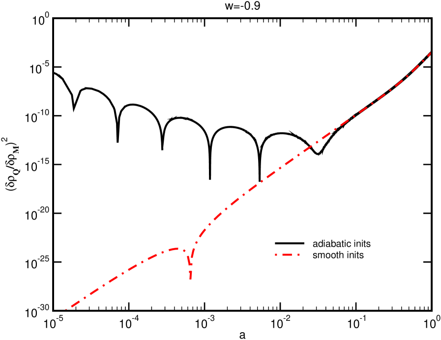
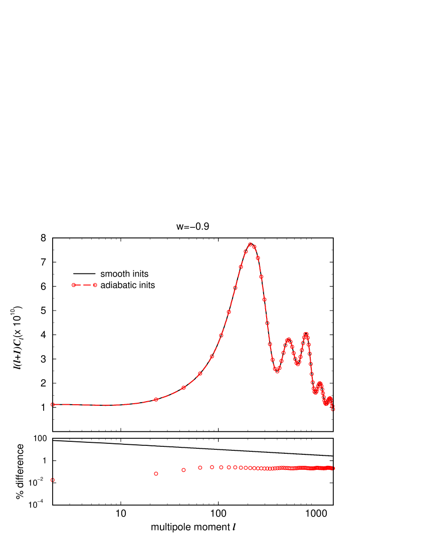
Figure 4: The figure in the left panel shows the evolution of the ratio of energy in $Q$ fluctuations to that in matter fluctuations $(\frac{\delta\rho_{Q}}{\delta\rho_{M}})^{2}$ at $k=10^{-4}Mpc^{-1}$ for both smooth initial conditions (inhomogeneous solution) and adiabatic initial conditions at $w=-0.9$. The figure in the right panel shows the corresponding CMB power spectra as a function of multipole moment. Plotted below the power spectrum is the percentage residual of the power spectrum for adiabatic initial conditions from smooth ones, compared to the fractional cosmic variance ($100\times{\Delta C_{\ell}\over C_{\ell}}$, plotted as a black line). The anisotropy change in going from smooth to adiabatic initial conditions is well below the variance

In the left panel of Figure 4, we compare the evolution of the ratio $\delta\rho_{Q}/\delta\rho_{m}$ at large wavelength ($k=10^{-4}Mpc^{-1}$) for smooth and adiabatic initial conditions, at $w=-0.9$. We see that the evolution of the ratio for the smooth case tracks the power law rise of the inhomogeneous solution to its present-day value. The magnitude of the ratio at last scattering ($a\sim 10^{-3}$) is much larger in the adiabatic case than in the smooth case, corresponding to the dominance of the homogeneous solution over the inhomogeneous one. Still, $\delta\rho_{Q}/\delta\rho_{m}$ remains far below unity in all epochs for the adiabatic case.

We plot the effect on the CMB anisotropy at $w=-0.9$ in the right panel of the figure, for both the smooth and adiabatic initial conditions. Below the spectra is plotted the absolute value of the residual, or the percentage difference of the power spectrum in the model with adiabatic initial conditions compared to the model with smooth initial conditions. We also plot the fractional cosmic variance. Residuals smaller than the variance cannot be observationally measured. As can be seen from the figure, the anisotropy for the adiabatic case at $w=-0.9$ is not observationally distinguishable from the smooth case within cosmic variance. While the addition of the homogeneous solution to the inhomogeneous one does increase the ratio $\delta\rho_{Q}/\delta\rho_{m}$ by many orders of magnitude, the increase is not enough, even at $w=-0.9$, to alter the CMB power spectrum.

Figure 5: The figure compares the evolution of the ratio $(\frac{\delta\rho_{Q}}{\delta\rho_{M}})^{2}$ for both adiabatic (${\sf F}=1$) and artificially amplified (${\sf F}=10^{4}$ and ${\sf F}=10^{5}$) initial conditions for the $w=-0.9$ model from Figure 3. The ratio is plotted for wave number $k=10^{-4}Mpc^{-1}$. We also plot a solid horizontal line to indicate a ratio of magnitude unity. Notice that the amplification prolongs the domination of the homogeneous solution, and the resultant closeness of the energy density ratio to unity.

If there is to be a distinguishable imprint of a change in initial conditions on the CMB anisotropy, the energy density in quintessence fluctuations must increase drastically so that $\delta\rho_{Q}/\delta\rho_{m}$ is of order unity at last scattering. Let us estimate how large the initial amplitude of $\delta\rho_{Q}/\rho_{Q}$ must be in order to have a distinguishable effect by artificially multiplying adiabatic initial conditions by a factor ${\sf F}$, and then comparing the result to the results for smooth initial conditions. We want to show that ${\sf F}$ must be quite large in order to have any detectable effect on the CMB anisotropy. In Figure 5 we display the evolution of $\delta\rho_{Q}/\delta\rho_{m}$ in the $w=-0.9$ model, for initial conditions that are adiabatic (${\sf F}=1$), and for initial conditions ${\sf F}=10^{4}$ and ${\sf F}=10^{5}$ times the adiabatic initial conditions. The ratio is plotted at a wavelength longer than the horizon today, $k=10^{-4}Mpc^{-1}$. In the case of amplified initial conditions, the homogeneous solution is larger, and thus it takes until very recent epochs for the inhomogeneous solution to become comparable to the homogeneous solution. The amplification of the initial conditions by ${\sf F}=10^{4}$ makes $\delta\rho_{Q}/\delta\rho_{m}$ larger than unity initially, and the dominance of the homogeneous solution keeps it close to, but smaller than unity at last scattering. An amplification by ${\sf F}=10^{5}$ makes the ratio to be of order unity at last scattering, which will leave an imprint on the CMB anisotropy.

To understand these effects from the perspective of the value of ${\delta\rho_{Q}\over\rho_{Q}}$, we need to obtain the value of the matter fluctuation at the initial hyper-surface ($a\sim 10^{-8}$). Since COBE normalization sets the amplitude of the matter fluctuation on re-entry to be ${\delta\rho_{m}\over\rho_{m}}\sim 10^{-5}$, we find from Eqn. 20 that $\Big{(}{\delta\rho_{m}\over\rho_{m}}\Big{)}_{init}\sim 10^{-16}$ in the synchronous gauge. The ratio of $\Big{(}{\delta\rho_{Q}\over\rho_{Q}}\Big{)}_{init}$ to $\Big{(}{\delta\rho_{m}\over\rho_{m}}\Big{)}_{init}$ is set either by imposing smooth or adiabatic initial conditions. In the former case we have $\delta\rho_{Q}/\rho_{Q}=0$ and so the ratio is zero. In the latter case, the ratio can be obtained by combining Eqns. 25 and 26 with the scale-factor dependence of $\rho_{m}$ and $\rho_{Q}$. The absolute value of this ratio ranges from $\sim 10^{-1}$ at $w=0$ to $10^{22}$ at $w=-0.9$. In other words, for $w$ closer to -1, ${\delta\rho_{Q}\over\rho_{Q}}$ is initially quite large. Yet there is no observable difference in anisotropy, as can be seen from Figure. 4, between the cases of smooth and adiabatic initial conditions. The amplitude of the homogeneous fluctuations swiftly declines and both the above ratio, and consequently $\delta\rho_{Q}/\delta\rho_{m}$ are much smaller than one by last scattering. Thus there is no observable change in the CMB anisotropy. It is only when the initial conditions are amplified by $F=10^{5}$ (so that $\Big{(}{\delta\rho_{Q}\over\rho_{Q}}\Big{)}\sim 10^{11}$ at the initial hyper-surface) that the steep decline cannot offset the initially large value by the epoch of last scattering, and there is any observable effect on the CMB. Of course, this large value of ${\sf F}$ is physically unrealistic, many orders of magnitude greater than what is expected from inflation, for example. Also, for such extreme values of ${\sf F}$, the linear approximation used in CMB analysis is invalid. This exercise shows clearly that we can ignore the initial conditions on the quintessence fluctuations for all reasonable models.

Figure 6: The figure depicts the CMB power spectrum as a function of multipole moment for two of the models of Figure 3 with $w=-2/3$ and $w=-0.9$. The power spectra are plotted for a series of cases with artificially amplified initial conditions, and for the corresponding model with adiabatic initial conditions. Also shown in the lower panel is the absolute value of the percentage residual of the amplified cases from the adiabatic case, as compared to the fractional cosmic variance (black line). At $w=-2/3$, an amplification of the adiabatic initial conditions even by ${\sf F}=10^{5}$, is not enough to make an observable change in the CMB power spectrum. On the other hand, in the $w=-0.9$ case, the power spectrum for the same value of ${\sf F}$ is markedly different.

In Figure 6, we plot the numerically computed power spectra at $w=-2/3$ and $w=-0.9$ for adiabatic and amplified initial conditions. The amplification is by factors of ${\sf F}=10^{2}$, $10^{4}$ and $10^{5}$ times the adiabatic initial conditions. Below the spectra, we plot the residuals with respect to the adiabatic model.

We see that at $w=-2/3$, the power spectrum in the amplified models is identical to that in the adiabatic model, even for ${\sf F}=10^{5}$. For $w=-0.9$, an amplification by a factor of $10^{2}$ leads to no distinguishable changes in the anisotropy. On the other hand, an amplification by ${\sf F}=10^{4}$ weakly suppresses the Doppler peak and creates changes in the anisotropy at some multipoles. The ratio of energy in quintessence fluctuations to energy in matter fluctuations for ${\sf F}=10^{4}$ is of the order $\sim 10^{-2}$-$10^{-1}$ at last scattering, as can be seen in Figure 5, and the residual anisotropy is barely smaller than the cosmic variance. Thus, the effects on the CMB are not large enough to be observationally distinguished. Amplification of the initial conditions in the $w=-0.9$ case by a factor of $10^{5}$ raises the amplitude of the homogeneous solutions sufficiently that ${\delta\rho_{Q}\over\delta\rho_{m}}\sim 1$ at last scattering. For equations of state even closer to -1, smaller amplification factors are required to make a measurable difference in the CMB anisotropy. However, the amplification is still large and unphysical. For example, even at $w=-0.999$, an amplification by ${\sf F}=10^{3}$ is required to create an observable effect.

6 Conclusions

We studied in this paper a large class of quintessence models with light fields and sound speed $c_{s}^{2}\sim 1$ at small wavelengths, which have the property that they can be well approximated by constant equation of state, $w$. The evolution of the fluctuations in these models was obtained by numerical integration and explained by approximate analytic solutions to the fluctuation equation at large wavelengths. Our central result is that the CMB anisotropy in such models is insensitive to initial conditions on the quintessence fluctuations for smooth and adiabatic initial conditions . For $w=-0.9$, the CMB anisotropy is insensitive in the large range of initial conditions $\Big{(}{\delta\rho_{Q}\over\rho_{Q}}\Big{)}_{init}<10^{11}\,(F=10^{5})$ for $\Big{(}{\delta\rho_{m}\over\rho_{m}}\Big{)}\sim 10^{-5}$ at horizon re-entry. Secondly, the sensitivity increases as $w$ approaches -1. At $w=-0.999$, the range reduces to $\Big{(}{\delta\rho_{Q}\over\rho_{Q}}\Big{)}_{init}<10^{9}\,(F=10^{3})$. However, physically reasonable models such as those based on inflation and ekpyrosis do not produce such large values of ${\delta\rho_{Q}\over\rho_{Q}}$, and the ratio of energy in quintessence fluctuations to that in matter fluctuations is much smaller than unity. Hence, we do not anticipate that the CMB anisotropy will be sensitive to initial conditions in realistic cases. The same analytical arguments made in this paper carry over to the more general quintessence models in which $w$ is more strongly time dependent or $c_{s}^{2}\neq 1$ at small wavelengths. However, the precise numerical lower bound on the initial conditions required to imprint a distinguishable effect on the CMB anisotropy has to be worked out on a case by case basis.

This work was supported by DOE grant DE-FG02-95ER40893 (RD), NSF grant PHY-0099543 (RRC), and DOE grant DE-FG02-91ER40671 (PJS).

References

- [1] L. Wang, R. R. Caldwell, J. P. Ostriker, and P. J. Steinhardt, Astrophys.J. 530, 17-35 (2000), astro-ph/9901388; N. Bahcall, J.P. Ostriker, S. Perlmutter, P. J. Steinhardt, Science 284, 1481-1488 (1999), astro-ph/9906463.
- [2] J.P. Ostriker and P.J. Steinhardt, Nature 377, 600 (1995); Michael S. Turner, “The case for Lambda CDM” in Critical Dialogues in Cosmology, ed. Neil Turok, (World Scientific: Singapore, 1997).
- [3] P.J. Steinhardt, Nature 382, 768 (1996).
- [4] R.R. Caldwell, R. Dave, and P.J. Steinhardt, Phys. Rev. Lett. 80, 1582 (1998), astro-ph/9708069.
- [5] P. T. Viana and A. R. Liddle, Phys. Rev. D 57, 674 (1998), astro-ph/9708247.
- [6] F. Perrotta, C. Baccigalupi, Phys.Rev.D 59 (1999) 123508
- [7] P. Brax, J. Martin, A. Riazuelo, Phys.Rev.D 62 (2000) 103505
- [8] D. Spergel and U.L. Pen, Astrophys.J. 491, L67-L71 (1997), astro-ph/9611198.
- [9] N. Weiss, Phys. Lett. B 197, 42 (1987).
- [10] C. Wetterich, Astron. Astroph. 301, 321 (1995); J.A. Frieman, et al. Phys. Rev. Lett. 75, 2077 (1995); K. Coble, S. Dodelson, and J. Frieman, Phys. Rev. D 55, 1851 (1995).
- [11] P.G. Ferreira and M. Joyce, Phys. Rev. Lett. 79, 4740 (1997), astro-ph/9707286; P.G. Ferreira and M. Joyce, Phys. Rev. D 58, 023503 (1998), astro-ph/9711102.
- [12] E. J. Copeland, A.R. Liddle, and D. Wands, Phys. Rev. D 57, 4686 (1998).
- [13] P. J. Steinhardt, L. Wang, and Ivaylo Zlatev, Phys.Rev.Lett. 82, 896-899 (1999), astro-ph/9807002; P. J. Steinhardt, L. Wang, I. Zlatev, Phys.Rev. D 59, 123504 (1999), astro-ph/9812313.
- [14] C. Armendariz-Picon, V. Mukhanov, P.J. Steinhardt, Phys.Rev.Lett. 85, 4438-4441 (2000), astro-ph/0004134.
- [15] U. Seljak and M. Zaldarriaga, Astrophys.J. 469, 437-444 (1996), astro-ph/9603033.
- [16] Rahul Dave, Ph. D. Thesis, University of Pennsylvania, Philadelphia, 2002.
- [17] C.P. Ma and E. Bertschinger, Ap. J. 455, 7 (1995).
- [18] J.A. Frieman, C.T. Hill, and R. Watkins, Phys. Rev. D 46, 1226 (1992); J.A. Frieman, C.T. Hill, A. Stebbins, and I. Waga, Phys. Rev. Lett. 75, 2077 (1997).
- [19] J.J. Halliwell, Phys. Lett. B 185, 341 (1987); Edmund J. Copeland, Andrew R. Liddle, and David Wands, Phys. Rev. D 57, 4821 (1998), gr-qc/9711068.
- [20] P. J. Steinhardt, astro-ph/9502024.
- [21] B. Ratra and P.J.E. Peebles, Phys. Rev. D 37, 3406 (1988); P.J.E. Peebles and B. Ratra, Ap. J. Lett. 325, 17 (1988).
- [22] Joel K. Erickson, R.R. Caldwell, Paul J. Steinhardt, C. Armendariz-Picon, V. Mukhanov, astro-ph/0112438