A statistical study of binary and multiple clusters in the LMC

Based on the Bica et al. (bica (1999)) catalogue, we studied the star cluster system of the LMC and provide a new catalogue of all binary and multiple cluster candidates found. As a selection criterion we used a maximum separation of $1\aas@@fstack{\prime}4$ corresponding to 20 pc (assuming a distance modulus of 18.5 mag). We performed Monte Carlo simulations and produced artificial cluster distributions that we compared with the real one in order to check how many of the found cluster pairs and groups can be expected statistically due to chance superposition on the plane of the sky. We found that, depending on the cluster density, between $56\%$ (bar region) and $12\%$ (outer LMC) of the detected pairs can be explained statistically. We studied in detail the properties of the multiple cluster candidates. The binary cluster candidates seem to show a tendency to form with components of similar size. When possible, we studied the age structure of the cluster groups and found that the multiple clusters are predominantly young with only a few cluster groups older than 300 Myr. The spatial distribution of the cluster pairs and groups coincides with the distribution of clusters in general; however, old groups or groups with large internal age differences are mainly located in the densely populated bar region. Thus, they can easily be explained as chance superpositions. Our findings show that a formation scenario through tidal capture is not only unlikely due to the low probability of close encounters of star clusters, and thus the even lower probability of tidal capture, but the few groups with large internal age differences can easily be explained with projection effects. We favour a formation scenario as suggested by Fujimoto & Kumai (fk (1997)) in which the components of a binary cluster formed together and thus should be coeval or have small age differences compatible with cluster formation time scales.

1 Introduction

The first systematic work on binary clusters in the Magellanic Clouds started approximately a decade ago. The first catalogue of binary star clusters in the LMC was presented by Bhatia & Hatzidimitriou (bh (1988)) and Bhatia et al. (brht (1991)) who surveyed the cluster system (consisting of 1200 objects known at that time) and listed 69 binary cluster candidates. Their selection criterion was a maximum separation between the components of a proposed pair of approximately 18 pc (assuming a distance modulus of 18.4 mag). Following Page (page (1975)), out of these 69 double objects only 31 can be explained as optical pairs, i.e., clusters that appear as close pairs on the plane of the sky due to projection effects. Ages were available only for some of the clusters and suggested that the pairs are young (between $10^{7}$ to a few $10^{8}$ yr), consistent with expected time scales for merger or disruption of binary clusters (Bhatia bhatia (1990)).

In the following years, more studies on binary cluster candidates were performed but concentrated mainly on one or a few individual objects in order to establish their binarity (Kontizas et al. kkx (1989), Lee lee92 (1992), Bhatia bhatia92 (1992), Kontizas et al. kkm (1993), Vallenari et al. vafcom (1994), Hilker et al. hrs (1995), Grebel gr97 (1997), Vallenari et al. vbc (1998), Leon et al. lbv (1999), Dieball & Grebel dg (1998, 2000), Dieball et al. dgt (2000)). Few theoretical studies concerning formation, gravitational interaction and dynamical evolution of binary clusters are available (Sugimoto & Makino sm (1989), Bhatia bhatia (1990), Fujimoto & Kumai fk (1997), de Oliveira et al. dodb (1998), Theis theis (1998)).

However, since the investigation of Bhatia & Hatzidimitriou (bh (1988)) and Bhatia et al. (brht (1991)) many more clusters have been discovered in the LMC. Thus, it is time to perform a new study on the nowadays better known LMC cluster system, aiming at the question of how many close cluster pairs exist and how many of these might be explained as chance superpositions.

Recently, Pietrzyński & Udalski (2000b ) provided a new but spatially limited catalogue of multiple cluster candidates in the LMC. They based their studies on the OGLE (see Udalski et al. ogle (1992)) dataset which covers 5.8 square degrees of the inner part of the LMC and contains 745 star clusters (Pietrzyński et al. puk (1999)). Out of these, a total of 100 multiple cluster candidates with a maximum separation of 18 pc, assuming a distance modulus of 18.24 mag, were selected. The cluster groups consisted of 73 pairs, 18 triple systems, 5 systems containing four components, 1 with five and 3 systems with six clusters. Assuming that all 745 clusters are distributed uniformly in the 5.8 square degree region and adopting the same statistical approach as Bhatia & Hatzidimitriou (bh (1988)), 51 chance pairs can be expected. A more detailed investigation of the cluster distribution led to nearly the same result of 53 random pairs. The number of all detected candidates is 153 and thus significantly larger than expected from chance superposition. Ages for the components were taken from Pietrzyński & Udalski (2000a ). 102 components are coeval, 53 have very different ages, and most objects are younger than 300 Myr with a peak at 100 Myr. This suggests that most of the multiple clusters have a common origin and are quite young objects.

A catalogue of multiple cluster candidates in the SMC was published by Pietrzyński & Udalski (pu_smc (1999)), containing 23 binary and 4 triple cluster candidates. A comparison of both the LMC and SMC binary cluster lists reveals that the distribution of the components’ separation, the fraction of cluster groups ($\approx$ 12 %) and their ages are very similar. The similar ages of the binary cluster candidates in both the LMC and SMC might be connected with the last close encounter between these two galaxies. De Oliveira et al. (2000b ) presented an isophotal atlas of 75 binary and multiple clusters (comprising 176 objects) from the Bica & Dutra (bd (2000)) catalogue of SMC clusters. Bica & Dutra (bd (2000)) included also new discoveries from the OGLE catalogue of SMC clusters (Pietrzyński et al. puk_smc (1998)). Investigating the isophotes of the binary and multiple cluster candidates, de Oliveira et al. (2000b ) found isophotal distortions, connecting bridges, or common isophotal envelopes for 25 % of the suggested multiple clusters. The authors interpreted this as signs of interaction between the components of a supposed binary or multiple cluster, in agreement with the findings from previous N-body simulations (de Oliveira et al. 2000a ). Ages for 91 out of the 176 clusters that are part of pairs or groups were investigated based on the OGLE $BVI$ maps. 40 clusters are in common with Pietrzyński & Udalski (pu_smc (1999)), and de Oliveira et al. (2000b ) found good agreement with the study of the OGLE group. Most clusters are young, and the age distribution shows a relevant peak around 200 Myr that can be attributed to the last close encounter between SMC and LMC. The components of groups with more than two members are younger than 100 Myr, which might be an indication that multiple clusters coalesce into binary or single clusters within this timescale. 55 % of the binary and multiple cluster candidates were found to be coeval. From this the authors concluded that tidal capture is a rare phenomenon.

In this paper, we present a statistical study of close pairs and multiple clusters in the LMC. We decided to base our analysis on the new, extended catalogue of stellar clusters, associations, and emission nebulae in the LMC provided by Bica et al. (bica (1999), hereafter BSDO). The authors surveyed the ESO/SERC R and J Sky Survey Schmidt films, checked the entries of previous catalogues and searched for new objects. The resolution of the measurements was $<4\arcsec$ (Bica & Schmitt bs (1995)). The resulting new catalogue unifies previous surveys and contains 6659 entries, out of which 3246 are new discoveries that are not mentioned in previous catalogues and lists. Thus, the BSDO catalogue can be considered as the so far most complete catalogue of LMC stellar clusters and associations. We restricted our study to bound stellar systems, which means that we selected only objects which are categorized as “C”-type (cluster-type), and left out associations and emission nebulae, which are not of interest in the context of the present study. This reduces the number of objects found in the BSDO catalogue from a total of 6659 to 4089.

Based on this catalogue, we performed a statistical study of cluster pairs and groups and provide a complete list of all multiple cluster candidates in the LMC.

In the following sections, we address a number of questions: How many cluster pairs can be found with a projected separation of less than 20 pc between the components of a pair (Sect. 4)? Following Bhatia & Hatzidimitriou (bh (1988)) and Bhatia et al. (brht (1991)), we consider this to be a good selection criterion. Several cluster pairs may form a larger cluster group, e.g., if a component of a cluster pair is less than 20 pc distant from any component of another pair. In this way, three clusters may form a triple cluster, but they also might constitute three cluster pairs if each cluster is seen within 20 pc from each other cluster. How many “multiple” clusters, consisting out of more than two single objects, are present, and how many single clusters are involved in these pairs and groups (Sect. 4)? How many of these pairs and multiple systems can be expected statistically, and of how many individual components do they consist (Sect. 5)? Are there any correlations between the properties of the cluster systems such as ages, radii and separations between the components (Sect. 6)? What is the fraction of coeval pairs or groups compared with the number of multiple clusters whose internal age differences exceed the protocluster survival time (Sect. 6.4)? Does the percentage of coeval systems agree with the number of statistically expected groups (Sect. 6.4)? And finally, do our results favour or give hints at a specific cluster formation scenario (Sect. 7)? For instance, can cluster pairs be explained with statistically expected cluster encounters in the LMC, which lead to tidal capture and thus to bound pairs of different ages (see Sect. 3)? Or are the multiple cluster candidates predominantly found to be coeval, favouring the formation scenario of Fujimoto & Kumai (fk (1997)) or of Theis (theis (1998))?

2 Cluster density distribution

Looking at an optical image of the LMC, it is apparent that the stellar and cluster distribution is not uniform across this galaxy. One of the most striking features besides the prominent star-forming H ii regions is the LMC bar, a region of increased stellar density.

In Fig. 1 we plotted the angular distribution of all clusters listed in the BSDO catalogue. Again, the bar structure can easily be recognized. However, the clusters are not evenly distributed in the outer LMC. To make the structures of the cluster density distribution more apparent, Fig. 1 was smoothed with a Gaussian filter with a blur radius of 50 image pixels. The intensity scale of the resulting figure (Fig. 2) was reduced to 15 bins, the darkest shade indicating the highest cluster density. In this way, it is possible to get qualitative information about the density distribution, however, quantitative values of the cluster densities cannot be derived from the image’s greyscales alone. All steps were performed with the aid of common image processing tools (GIMP).

Regions of different cluster densities and their spatial extent can be seen in Fig. 2: Apart from the prominent bar structure, also the area surrounding the bar is densely populated with star clusters. To the north-east another region of enhanced cluster density is clearly visible, which coincides with LH 77 (Lucke & Hodge lh (1970)) in the supergiant shell LMC 4 (see e.g. Braun et al. braun (1997)) and the constellation Shapley III (McKibben Nail & Shapley mshapley (1953)). The outermost LMC areas show a considerable drop-off in the cluster density, which is already recognizable in Fig. 1.

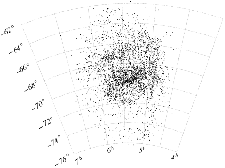
Figure 1: Angular distribution of all cluster-like objects derived from the BSDO catalogue. The bar structure is clearly visible

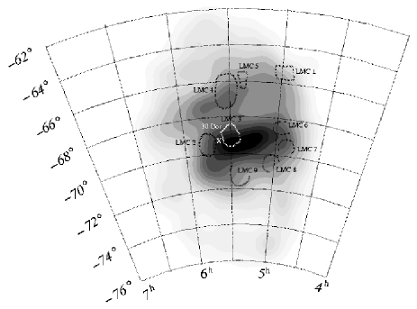
Figure 2: Density plot of all LMC clusters. The highest cluster density (black) coincides with the bar region. Please note that this picture provides qualitative information about the density distribution. No quantitative values of the cluster densities can be derived from the image’s greyscales alone. The location of the supergiant shells LMC 1 – LMC 9 are sketched (see Fig. 6, page 6, in Braun braundr (2001)). The position of 30 Doradus is marked with a white cross

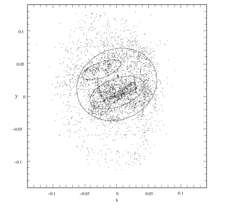
Figure 3: Cluster distribution plotted in cartesian coordinates. The regions that are selected on the basis of the cluster density plot are sketched

Due to the non-uniform distribution of the star clusters in the LMC, we decided to subdivide the BSDO catalogue into regions of equal cluster densities. It is a difficult task to find a suitable partition: it has to be small enough so that a (nearly) uniform distribution of clusters can be assumed but general density differences between larger areas must still be recognizable and may not be smeared out by a too small partition, and the regions have to be larger than the detection limit for cluster pairs and groups. Based on Fig. 2, we decided to split the input catalogue into five lists: the inner part of the LMC shows in general a higher concentration of star clusters, thus we first distinguish between an inner ellipse (which we call $E_{\rm inner}$) and an outer ring, the remaining outer LMC area which shows an overall low cluster density ($E_{\rm outer}$). Inside the inner ellipse, there are still regions of varying cluster frequencies. Thus, we further define an ellipse surrounding the bar (which we call $E_{\rm bar}$), a rectangular area that coincides with the bar itself (called “bar”), and an ellipse north-east of the bar corresponding to the location of LMC 4 ($E_{\rm north}$). All areas are disjunctive, i.e., if a selected region contains one or more selected ellipses or the bar, these “inner” areas are not considered in the following calculations and simulations, i.e., $E_{\rm bar}$ does not contain the bar, $E_{\rm inner}$ does not contain $E_{\rm bar}$ and $E_{\rm north}$ and so on.

For the following selections and Monte Carlo simulations it is suitable to transform the spherical coordinates of the catalogue entries ($\alpha$, $\delta$ coordinates) into cartesian coordinates ($x,y$) (see, e.g., Geffert et al. geffert (1997) and Sanner et al. sanner (1999)). The gnomonic projection was done via:

$$x = \frac{-\cos\delta\cdot\sin(15\cdot(\alpha-\alpha_{0}))}{\sin\delta\cdot\sin\delta_{0}+\cos\delta\cdot\cos\delta_{0}\cdot\cos(15\cdot(\alpha-\alpha_{0}))}$$ (1)

$$y = \frac{\sin\delta\cdot\cos\delta_{0}-\cos\delta\cdot\sin\delta_{0}\cdot\cos(15\cdot(\alpha-\alpha_{0}))}{\sin\delta\cdot\sin\delta_{0}+\cos\delta\cdot\cos\delta_{0}\cdot\cos(15\cdot(\alpha-\alpha_{0}))}$$ (2)

(van de Kamp vandekamp (1967)). We adopt $\alpha_{2000}=-69^{\circ}$ $45\arcmin$ and $\delta_{2000}=5^{h}$ $23\aas@@fstack{\prime}6$ as the central coordinates of the LMC (CDS data archive). Fig. 3 shows the cluster distribution in cartesian coordinates.

The selection criterion for clusters situated inside an ellipse with the semi major axes $a$ and $b$, central coordinates $x_{0}$ and $y_{0}$, and rotation angle $\phi$ is:

$$\left(\frac{(x-x_{0})\cdot\cos\phi+(y-y_{0})\cdot\sin\phi)}{a}\right)^{2}+$$

$$\left(\frac{(x-x_{0})\cdot\cos\phi-(y-y_{0})\cdot\sin\phi}{b}\right)^{2}\leq 1$$

The semi axes, central coordinates and the rotation angle for the selected ellipses are listed in Table 1. A helpful tool for selecting the bar region is the map of the LMC provided by Smith et al. (smith (1987), their Fig. 4) in which prominent features are sketched. The vertices that we choose to cut out the bar are listed in Table 2.

All selected areas are sketched in Fig. 3.

Table 1: Semi axes $a$ and $b$ (in units of the cartesian system), central coordinates $x_{0}$ and $y_{0}$ and the rotation angle $\phi$ for the selected ellipses for which uniform cluster densities are assumed (see Eq. 2)

Region $a$ $b$ $x_{0}$ $y_{0}$ $\phi$ $E_{\rm bar}$ 0.045 0.020 0.000 0.005 $20^{\circ}$ $E_{\rm north}$ 0.030 0.013 0.025 0.040 $20^{\circ}$ $E_{\rm inner}$ 0.065 0.055 0.002 0.018 $25^{\circ}$ $E_{\rm outer}$ 0.100 0.135 $-0.005$ 0.015 $0^{\circ}$

Table 2: Vertices defining the selected bar region

$x$ $y$ 0.0265 0.0212 0.0337 0.0119 $-0.0199$ $-0.0067$

3 Probability of tidal capture

The probability of close encounters between star clusters leading to a tidal capture is considered to be relatively small or even very unlikely (Bhatia et al. brht (1991)). However, van den Bergh (vdbergh (1996)) suggested that it becomes more probable in dwarf galaxies like the Magellanic Clouds due to the small velocity dispersion of the cluster systems. Furthermore, Vallenari et al. (vbc (1998)) proposed that interactions between the LMC and SMC might have increased the formation of star clusters in large groups in which the encounter rate and thus the formation of bound binary clusters is higher. This scenario is capable of explaining large age differences between cluster pairs which Leon et al. (lbv (1999)) refer to as the “overmerging problem”. In this section, we will determine the cluster encounter rates in our selected areas.

Inside the chosen regions we find 491 clusters in the bar, 863 in the remaining parts of $E_{\rm bar}$, 372 objects in $E_{\rm north}$, 1439 clusters in $E_{\rm inner}$ (without $E_{\rm bar}$ and $E_{\rm north}$), and 924 remaining entries in the outer region of the LMC. Assuming a distance modulus of 18.5 mag to the LMC, 1 pc corresponds to $1.999\cdot 10^{-5}$ units in our cartesian system. This leads to a length of 2710 pc and a width of 591 pc for the bar, and thus to a cluster density of $3\cdot 10^{-4}$ clusters${\rm\leavevmode\nobreak\ pc}^{-2}$. For $E_{\rm bar}$, the semi major axis corresponds to 2250 pc and its semi minor axis to 1000 pc, resulting in $863\mbox{ }{\rm clusters}/(A_{\rm E_{\it bar}}-A_{\rm bar})=1.6\cdot 10^{-4}$ clusters${\rm\leavevmode\nobreak\ pc}^{-2}$. Cluster densities for the other selected areas follow in an analogous manner: $1.2\cdot 10^{-4}$ clusters${\rm\leavevmode\nobreak\ pc}^{-2}$ for $E_{\rm north}$, $8\cdot 10^{-5}$ clusters${\rm\leavevmode\nobreak\ pc}^{-2}$ for $E_{\rm inner}$ (without the northern ellipse and the region surrounding the bar), and $1.2\cdot 10^{-5}$ clusters${\rm\leavevmode\nobreak\ pc}^{-2}$ for the outer ring $E_{\rm outer}$. Please note that, assuming an outer ring with limited boundaries and semi axes corresponding to 5000 pc and 6750 pc, the number of objects in $E_{\rm outer}$ amounts to 911. However, this does not alter the value of the outer cluster density.

The cluster density is highest in the innermost part of the LMC, the bar region, and it drops off by an order of magnitude towards the outer region. According to Vallenari et al. (vbc (1998)), cluster pairs can be formed by close encounters which result in the tidal capture of two clusters. The higher the cluster density, the higher the probability for close encounters, and thus the probability for the formation of cluster pairs or groups.

The cluster encounter rate can be determined following Lee et al. (lee95 (1995)):

$$\frac{{\rm d}N}{{\rm d}t}=\frac{1}{2}\cdot\frac{N-1}{V}\cdot\sigma\cdot v$$ (4)

where $N$ is the number of clusters, $V$ denotes the volume of the galaxy or, respectively, the part of the galaxy under investigation, $\sigma=\pi R^{2}$ is the geometric cross section of a cluster with radius $R$, and $v$ is the velocity dispersion of the cluster system of that galaxy. Typical cluster radii are about 10 pc. For the velocity dispersion of the cluster system we adopt 15 km $\mbox{s}^{-1}$ as quoted in Vallenari et al. (vbc (1998)). For the depth of the LMC, and thus for each selected area, we adopt 400 pc (Hughes et al. hughes (1991)). This leads to a cluster encounter rate of $20\cdot 10^{-10}\leavevmode\nobreak\ {\rm yr}^{-1}$ inside the bar. In the ellipse surrounding the bar, the northern region and the inner LMC region, the probability of close encounters is much lower by a factor of 2 to 4, namely $9\cdot 10^{-10}\leavevmode\nobreak\ {\rm yr}^{-1}$ in $E_{\rm bar}$, $7\cdot 10^{-10}\leavevmode\nobreak\ {\rm yr}^{-1}$ in $E_{\rm north}$, and $5\cdot 10^{-10}\leavevmode\nobreak\ {\rm yr}^{-1}$ in $E_{\rm inner}$. The lowest encounter rate is, as expected, in the outer ring with a value of $0.7\cdot 10^{-10}\leavevmode\nobreak\ {\rm yr}^{-1}$. This means that the probability of a close encounter between star clusters is $\approx 30$ times higher in the bar than in the outskirts of the LMC.

All results are summarized in Table 3.

The probabilities for cluster encounters are already very low. In addition, the probability of tidal capture depends on further conditions which will not be fulfilled during every encounter. Whether a tidal capture takes place or not depends strongly on the velocities of the two clusters with respect to each other, on the angle of incidence, whether sufficient angular momentum can be transferred, and whether the clusters are sufficiently massive to survive the encounter. Since only very few of these rare encounters would result in tidal capture, it seems unlikely that a significant number of young pairs may have formed in such a scenario.

Table 3: Semi axes $a$, $b$ in pc and number of clusters found in the selected regions, the resulting cluster densities and the encounter rate ${\rm d}N/{\rm d}t$. For the bar region, $a$ and $b$ do not denote semi axes, but the lengths of a rectangular area

Region $a$ [pc] $b$ [pc] $N_{\rm clusters}$ $\frac{{\rm clusters}}{{\rm\leavevmode\nobreak\ pc}^{2}}$ ${\rm d}N/{\rm d}t$ Bar (2710) (591) 491 $3\cdot 10^{-4}$ $20\cdot 10^{-10}{\rm yr}^{-1}$ $E_{\rm bar}$ 2250 1000 863 $1.6\cdot 10^{-4}$ $9\cdot 10^{-10}{\rm yr}^{-1}$ $E_{\rm north}$ 1500 $\mbox{ }\mbox{\,}650$ 372 $1.2\cdot 10^{-4}$ $7\cdot 10^{-10}{\rm yr}^{-1}$ $E_{\rm inner}$ 3250 2750 1439 $8\cdot 10^{-5}$ $5\cdot 10^{-10}{\rm yr}^{-1}$ $E_{\rm outer}$ 5000 6750 911 $1.2\cdot 10^{-5}$ $0.7\cdot 10^{-10}{\rm yr}^{-1}$

4 Numbers of cluster pairs and cluster groups

Table 4: Statistics about the cluster groups found in the selected regions. $N_{\rm tot}$ denotes all clusters found in the corresponding region, $N_{\rm cl}$ is the number of clusters involved in $N_{\rm pairs}$ pairs. The numbers of isolated pairs $N_{\rm 2}$, triple systems $N_{\rm 3}$, and so on can be found in the subsequent columns. Groups consisting of more than eight members do not occur

Region $N_{\rm tot}$ $N_{\rm cl}$ $N_{\rm pairs}$ $N_{\rm 2}$ $N_{\rm 3}$ $N_{\rm 4}$ $N_{\rm 5}$ $N_{\rm 6}$ $N_{\rm 7}$ $N_{\rm 8}$ Bar 491 228 166 59 22 5 – 4 – – $E_{\rm bar}$ 863 306 207 97 20 5 2 1 – 2 $E_{\rm north}$ 372 117 88 36 5 3 2 – – 1 $E_{\rm inner}$ 1439 371 247 131 19 5 4 2 – – $E_{\rm outer}$ 924 93 55 40 3 1 – – – – Sum 4089 1115 763 363 69 19 8 7 – 3 LMC total 4089 1126 770 366 69 19 9 7 – 3

As the selection criterion for binary cluster candidates we chose a maximum angular separation of $\leq 1\aas@@fstack{\prime}4$ corresponding to a projected distance of 20 pc (assuming a distance modulus of 18.5 mag) between the centres of a proposed cluster pair. This is nearly the same value that was used by Bhatia & Hatzidimitriou (bh (1988)), Hatzidimitriou & Bhatia (hb (1990)), and Bhatia et al. (brht (1991)). According to Bhatia (bhatia (1990)) and Sugimoto & Makino (sm (1989)), binary clusters with larger separations may become detached by the external tidal forces while shorter separations may lead to mergers.

Out of 491 clusters in the bar region, 228 objects can be found in double or even multiple systems. This amounts to $\approx 46\%$ of all bar clusters. We counted in total 166 pairs. However, two or more pairs may form a larger group, e.g., three star clusters may form up to three pairs if each cluster is seen within a projected distance of less than 20 pc from each other cluster. This means that the 166 pairs do not consist of 334 different single clusters but only of the 228 objects mentioned above. Hence we call only an isolated pair a possible binary system. In the bar 59 isolated pairs, 22 triple clusters and 9 larger groups with up to six members can be found.

The area surrounding the bar, $E_{\rm bar}$, is roughly half as densely populated with star clusters as the bar region itself. The percentage of clusters found in potential binary and multiple systems is still high, $\approx 35\%$ (306 objects), forming in total 207 pairs.

The cluster density in the northern region, $E_{\rm north}$, is nearly the same as in $E_{\rm bar}$, and approximately the same percentage of clusters ($\approx 31\%$ or 117 objects) can be found in 88 pairs which form 36 binary, 5 triple, and 6 larger systems.

In the remaining inner LMC region ($E_{\rm inner}$) the cluster density is lower by an order of a magnitude; however, still $\approx 26\%$ (371) of the clusters appear in potential binary and multiple systems.

In the outskirts of the LMC, the cluster density is the lowest, as is the number of clusters involved in pairs and groups: 93 “outer” clusters, i.e., $10\%$, form in total 55 pairs (40 binary, 3 triple and 1 quadruple systems).

The distribution of all cluster groups found in each selected area is summarized in Table 4 and illustrated in Fig. 6. The percentage of all clusters involved in the groups is indicated in Fig. 6, e.g., $24\%$ (or 118) of all clusters can be found in 59 binary systems in the bar.

Table 4 also lists the sum of all clusters and cluster pairs which result if the values for the different regions are added up. The last line of Table 4 gives the group statistics for the whole LMC without a division into separated areas. As can be seen, the sum of the individual group statistics differs from the statistics found for the total LMC. This is due to the fact that some multiple cluster candidates are located at or across the borders of the selected areas, so that they get divided into smaller groups or might even disappear as a cluster group through the division into different regions.

We caution that this statistical approach so far does not take into account possible age differences between clusters (which are mainly unknown). Also, we do not have any other information about the actual three-dimensional separation between the clusters.

5 Monte Carlo Simulations – how many pairs can be expected statistically?

In order to check how many of all the found pairs and multiple clusters can be expected statistically due to chance line-up, we performed statistical experiments:

For this purpose we developed C and C++ software which performs Monte Carlo simulations and analyses of the resulting random distribution.

The simulations are carried out in the cartesian system and we used the same selected areas as mentioned in Sect. 2. The same number of objects which were found based on the BSDO catalogue are now distributed randomly in each region, i.e., 372 objects are randomly spread in an ellipse with semi axes of 0.030 and 0.013 (or 1500 and 650 pc) for the inner, northern region $E_{\rm north}$; 491 objects are stochastically distributed in a rectangular area with lengths of $1.1822\cdot 10^{-2}$ and $5.4189\cdot 10^{-2}$ in units of the cartesian system (corresponding to 591 and 2710 pc) which denotes the LMC bar; 863 objects are arbitrarily placed in the space between the bar and the boundaries of the ellipse described with $E_{\rm bar}$ and so on. In this way, artificial cluster distributions are produced that can be compared with the true distribution in the LMC. To improve statistics this procedure was repeated 100 times for each region.

An example of an artificial cluster distribution is plotted in Fig. 4. The inner part of the LMC, including the bar and the northern region corresponding to LMC 4, is well represented. However, there is a sharp drop-off in the cluster density in the outskirts. The cluster density in the LMC is low in its outer regions, however, the decrease between the inner and outer region ($E_{\rm inner}$ and $E_{\rm outer}$) is smoother (see Fig. 3). Fig. 5 displays the density distribution of the artificial cluster system. Compared with Fig. 2 all prominent features are well represented.

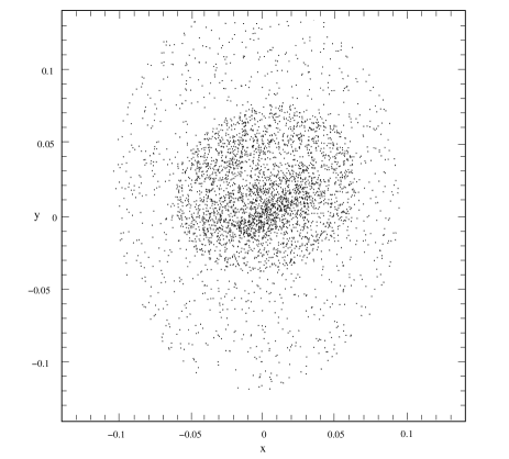
Figure 4: Example of one of the artificial cluster distributions that was created using Monte Carlo simulations. The distribution is plotted in cartesian coordinates and can be compared with Fig. 3, which shows the real LMC cluster distribution

Figure 5: Density distribution of the artificial cluster system represented in Fig. 4

The number of chance pairs and groups in our simulated cluster distributions as well as the number of single objects involved in these groups was counted and compared with our findings based on BSDO. As pointed out in the previous sections, two objects are considered as a pair and thus will be included in our list of random pairs or groups if their separation is 20 pc ($3.9979\cdot 10^{-4}$ in units of the cartesian system) at maximum.

Out of 491 random objects in the bar region, $\approx 156\pm 14$ can be found in $\approx 94\pm 10$ pairs. In reality, the LMC bar comprises 166 pairs which is nearly twice the amount of what we can expect statistically. However, a closer look at the group statistics reveals that of the 59 binary systems found in the real LMC bar cluster distribution, $55\pm 6$ isolated pairs can be explained as chance pairs based on our simulations, i.e., these numbers agree within the uncertainties. A discrepancy between found and expected figures is more apparent when groups with three or more members are considered. Out of 22 triple systems, only $\approx 11\pm 4$ (i.e., $\approx 50\%$) can be explained with chance superpositions. The number of actually found groups containing four members is twice as much as expected (5 found, 2.49 expected). 4 groups with six members are found, however, their random formation is very unlikely (0.21).

The statistically expected number of chance pairs and groups are summarized in Table 5 for all regions. A graphical display of our results can be found in Fig. 6. The numbers of the cluster groups actually found in the LMC regions are also indicated in Fig. 6 (see also Sect. 4) so that the results of both the real and the simulated cluster distribution can easily be compared.

In the remaining space of $E_{\rm bar}$, 207 pairs are actually found, but only $84\pm 9$ ($\approx 41\%$) of them can be explained statistically. Out of 97 isolated pairs, $\approx 66\%$ can be ascribed to chance superpositions. 20 triple systems are found, but only $7\pm 2$ can be expected. Again, for larger groups the discrepancy increases.

In the northern region, $E_{\rm north}$, $33\%$ ($\approx 29\pm 6$ pairs) of the 88 ones found can be expected due to chance line up.

For the remaining part of the inner LMC ($E_{\rm inner}$), $\approx 29\%$ of all pairs are explainable on a statistical basis.

Table 5: Statistics about the cluster groups found in the simulated regions. The standard deviations are given in brackets. Column labels are as in Table 4

Region $N_{\rm tot}$ $N_{\rm cl}$ $N_{\rm pairs}$ $N_{\rm 2}$ $N_{\rm 3}$ $N_{\rm 4}$ $N_{\rm 5}$ $N_{\rm 6}$ $N_{\rm 7}$ $N_{\rm 8}$ Bar 491 156.39 94.18 54.64 11.13 2.49 0.47 0.21 0.01 0.01 (14.28) (9.83) (6.11) (3.67) (1.72) (0.67) (0.46) (0.10) (0.10) $E_{\rm bar}$ 863 152.37 84.05 63.59 7.00 0.89 0.10 0.01 0.01 – (15.57) (9.23) (7.20) (2.40) (0.84) (0.30) (0.01) (0.01) – $E_{\rm north}$ 372 52.72 28.83 22.44 2.18 0.30 0.02 – – – (10.24) (5.70) (4.41) (1.34) (0.56) (0.14) – – – $E_{\rm inner}$ 1439 136.51 71.50 62.53 3.53 0.19 0.02 – – – (16.20) (8.61) (7.59) (1.77) (0.44) (0.14) – – – $E_{\rm outer}$ 911 13.12 6.58 6.53 0.02 – – – – – (5.16) (2.55) (2.54) (0.14) – – – – – Sum 4076 511.11 285.14 209.73 23.86 3.87 0.61 0.22 0.02 0.01 (28.82) (14.92) (12.12) (5.10) (2.16) (0.85) (0.48) (0.14) (0.20) Total 4076 515.58 288.01 211.32 24.19 3.97 0.63 0.22 0.02 0.02 (26.02) (15.35) (12.2) (4.96) (2.49) (0.80) (0.46) (0.14) (0.14)

The outer LMC is approximated by a ring (see Sect. 3) in which 911 objects are randomly distributed. These are 13 objects less than are actually found outside of $E_{\rm inner}$. However, these 13 clusters are located so far outside that a region which includes all these objects cannot be assumed to have an overall constant cluster density. No cluster pairs are among these outer objects so that they do not need to be included in our statistics. 55 cluster pairs are found in $E_{\rm outer}$, but only $\approx 12\%$ of them ($\approx 7\pm 3$ pairs) can be explained due to chance line-up. Though there is a low probability for a triple system (0.02), no larger group occurred in our simulations.

Table 5 also lists the sum of all cluster pairs and groups that can be expected if the figures for all regions are added up. The last line of Table 5 gives the group statistics for an entire artificial LMC, i.e., the experiments for the selected regions are put together. Again, as was already noticed for Table 4, the statistics show slight differences since some chance pairs and groups are located across the rims of the selected regions. However, the differences are much smaller than for the “real” LMC (Table 4). Comparing the results with Table 4 it can be seen that approximately $37\%$ ($288\pm 15$) of the found 770 cluster pairs can be expected due to spatial superposition. Approximately $58\%$ ($211\pm 12$) of all 366 binary cluster candidates can be expected statistically. The discrepancy between found and expected cluster groups increases for larger groups.

For each region, the number of pairs that can be expected due to random superposition is much lower than the number of pairs that are actually found: Between $56\%$ (in the bar region) and $12\%$ (in the outer LMC ring) of all detected pairs can be explained statistically. It seems that the discrepancy between found and expected pairs also depends on the cluster density of the region, i.e., in the densest bar region the percentage of pairs that can be explained statistically is also the highest, while it is the lowest in the region with the lowest cluster density (the outer ring). It is striking that especially large cluster groups with more than four members scarcely occur in any of the artificial cluster distributions.

Figure 6: Histogram of the number of cluster groups found in the selected regions of different cluster densities. The solid line denotes the number of groups detected in the real cluster distribution, while the dashed line indicates the number of cluster systems which can be expected statistically. The percentage of the clusters involved in the groups of different member size is also given. See Sect. 5 for details

6 Properties of the multiple clusters

6.1 Separations between the components of the cluster pairs

The distribution of the projected centre-to-centre separations of all LMC cluster pairs is displayed in Fig. 7 (solid line). Two peaks around 6 pc and approximately 15 pc are apparent. The peak around 6 pc as well as the subsequent decline around 9 pc are independent of binning. The median separation of the sample is $11.9\pm 5.2$ pc, the mode (the most probable value) is $6.3$ pc. The number of cluster pairs with a separation of 10 pc and larger increases, but seems to level off or even decrease again at separations of 18 pc and larger.

Assuming a uniform distribution of separations we calculate a median of $43\pm 9$ clusters per bin. Note that we took into account only separations between 3 and 20 pc since the number of pairs observed with very small separations is very low. This might very well be a selection effect since clusters with such small separations might not be detected because they are overlapping and thus appear as one single object. Figure 7 shows a maximum at approx. 6 pc with 45 pairs, a minimum at 9 pc with 31 pairs, and again a maximum at 17 pc with 55 pairs. The minimum and the second maximum are significantly below and over the median figure.

To constrain our presumption we performed a KMM (“Kaye’s mixture model”, see Henriksen et al. henriksen (2000)) test. Basically, mixture modelling is used to detect clusterings in datasets and to assess their statistical significance. The KMM fits a user-specified number of Gaussians to a dataset. The algorithm iteratively determines the best positions of the Gaussians and assigns to each data point a maximum likelyhood estimate of being a member of the group. It also compares the fit with the null-assumption, that is a single Gaussian fit to the dataset, and evaluates the improvement over the null-assumption using a “likelyhood ratio test statistic”. The algorithm is described in detail in Ashman et al. (ashman (1994)). The user has to provide as an input the number of data points, an initial guess for the number of groups, their positions, and sizes. A great advantage of KMM is that it works on the data themselves and is not applied to the histogram, thus it is completely independent of binning and not affected by any subjective visual impression.

For our first guess, we assumed two distributions with positions (i.e., the mean of the Gaussians) at 6 and 15 pc, 4 pc as the standard deviation of the Gaussians, and a mixing proportion of 0.4 and 0.6 for the two groups. The number of data points assigned to each group by KMM is 325 and 440 with estimated correct allocation rates of 0.914 and 0.944 for the two groups. The estimated overall correct allocation rate is 0.931. The estimated means of the two groups are 6.644 and 15.442 (close to our assumed positions). The hypothesis that the distribution can be fitted by a single Gaussian is rejected with more than 99 % confidence.

It might be possible that the underlying distribution is best described with three Gaussians. Our input guess for this case was means at 6, 13, and 18 pc, a common standard deviation of 3, and mixing proportions of 0.4, 0.3, and 0.3. The KMM assigns 239, 239, 287 members to each group, with allocation rates of 0.936, 0.845, and 0.925 and an overall correct allocation rate of 0.903. The KMM estimated positions are at 5.368, 11.599, and 17.043. Again, the null-assumption is rejected with more than 99 % confidence. Compared to our first, two-Gaussian guess, the KMM estimate for the overall correct allocation rate is smaller. We conclude that the distribution is better described with a two-Gaussian distribution.

Figure 7: Distribution of separations for all cluster pairs (solid line) found in the LMC. The distribution seems to be bimodal with peaks around approximately 6 and 15 pc and with a decrease around 10 pc. The dashed line denotes cluster pairs in which both components have diameters larger than 7 pc, while the dotted line represents cluster pairs with diameters smaller than 7 pc. The error bars are calculated as $\pm\sqrt{N}$

Bhatia & Hatzidimitriou (bh (1988)) investigated the separations of their 69 proposed binary clusters and found a bimodal distribution with peaks around 5 and 15 pc, similar to our findings if a two-Gaussian distribution is assumed. Bhatia et al. (brht (1991)) further suggested a more uniform distribution for cluster pairs in which both clusters have diameters larger than 7 pc. However, a uniform distribution for large clusters can be explained in the following way: the larger the components of a cluster pair, the larger the probability that both clusters are overlapping and may not be detected as a cluster pair but as only one single large cluster. It is likely that the catalogue is not complete concerning cluster pairs in which both clusters are large but have a small separation.

Based on our catalogue of binary and multiple cluster candidates, we reinvestigated the distribution of separations for cluster pairs in which both components have diameters either larger or smaller than 7 pc. The dashed line in Fig. 7 denotes pairs consisting of large clusters while the dotted line stands for pairs with small components. Indeed, the bimodal distribution is most apparent for small components and seems to be peaked around approximately 5 and 15 pc, in agreement with the findings of Bhatia et al. (brht (1991)). For pairs consisting of large clusters, a bimodal distribution is not as apparent, but cannot be neglected either. We cannot confirm a uniform distribution of separations for pairs with large clusters.

A general increase in the number of pairs as a function of separation is obvious from Fig. 7. This increase can be expected because cluster pairs with larger separations between the components can more easily be detected than close couples of clusters which might overlap and thus “merge” into one single cluster. Besides, the probability of finding another cluster increases with increasing separation (and thus increasing area).

On the other hand, for a given separation between cluster pairs, we expect to find an increase in the number of binary cluster candidates towards smaller separations since the “projected” separations are smaller than the real one. This might explain the first peak around 6 pc in the distribution of separations. The decrease towards separations smaller than 6 pc can be expected since clusters with small separations likely overlap and thus are difficult to detect.

Consequently, the dip around 9 – 10 pc might be interpreted as a balance between the effects that lead to an increase in the number of cluster pairs towards either smaller or larger separations.

6.2 Size distribution

The size distribution of clusters that are part of cluster pairs or groups is displayed in the upper diagram of Fig 8. Most components of the cluster pairs are small. They have diameters between $0.2\arcmin$ ($\approx 3$ pc) and $1\aas@@fstack{\prime}5$ ($\approx 22$ pc) with a clear peak at $0\aas@@fstack{\prime}45$ ($\approx 6.6$ pc). The median diameter of the sample is $0\aas@@fstack{\prime}57\pm 0\aas@@fstack{\prime}26$ ($\approx 8.5\pm 3.8$ pc), the mode is at $0\aas@@fstack{\prime}48$ ($\approx 7$ pc). Only a few clusters have diameters larger than $1\aas@@fstack{\prime}8$ ($\approx 26$ pc). However, in spite of our selection criterion of a separation of 20 pc, we still find three clusters with diameters larger than 40 pc ($2\aas@@fstack{\prime}7$). This means that their companion cluster is embedded within their circumference. These clusters are NGC 1850 (or BRHT 5 a) with its companions NGC 1850 A and BRHT 5 b (or H88-159), and NGC 2214 which appears in the BSDO catalogue as two entries, namely NGC 2214 w and NGC 2214 e.

The lower diagram in Fig. 8 shows the diameter distribution for all clusters found in the BSDO catalogue. Again, most clusters are rather small with a peak at $0\aas@@fstack{\prime}45$ or $\approx 6.6$ pc. The median diameter of the entire cluster sample is $0\aas@@fstack{\prime}62\pm 0\aas@@fstack{\prime}41$ ($\approx 9\pm 6$ pc) and the mode is $0\aas@@fstack{\prime}55$ or $\approx 8$ pc.

Both distributions (upper and lower figure) are qualitatively very similar.

The normalized ratio of the diameters of clusters that form a pair are plotted in Fig. 9. The median ratio of the sample is $0.73\pm 0.2$. The number of cluster pairs increases towards a size ratio of 0.5, but drops at a ratio larger than 0.5 and lower or equal than 0.55, and then increases again towards a ratio of 1. The number of pairs increases with larger ratios, which might indicate that binary clusters tend to form with components of similar sizes.

Figure 8: Size distribution of the clusters involved in pairs (upper diagram) and of all LMC clusters (lower diagram)

Figure 9: Diameter ratio of the components forming a cluster pair (solid line). The number of pairs increases with increasing ratio. The dotted line represents the distribution of ratios for scrambled diameters. See Sect. 6.2 for the details

The dotted line in Fig. 9 represents the size ratio of cluster pairs if all diameters are mixed and then randomly assigned to the pair members. To get reliable statistics we repeated this procedure 100 times. The number of pairs increases with increasing ratio, but seems to decrease again at ratios larger than 0.75, which confirms the impression that “true” binary clusters tend to form with components of similar sizes. Again, there is a peak at 0.5 and a following dip at ratios slightly larger than 0.5, though not as prominent as in the distribution of found ratios (solid line). However, a uniform distribution is not expected for statistical reasons: the diameters of the clusters in the BSDO catalogue are given in arc minutes in steps of $0\aas@@fstack{\prime}05$, i.e., the smallest diameter is $0\aas@@fstack{\prime}25$, the next one $0\aas@@fstack{\prime}3$ and so on. Since we consider mean diameters, we obtain discrete values with an increment of $0\aas@@fstack{\prime}025$. This means that some ratios are more probable than other ones, namely the unit fractions, which includes a ratio of $0.5=1/2$, while other ratios might result only few times in the distribution. For example, a ratio of $34/35$ can only result from three combinations of diameters in the given distribution of diameters, namely if both components of the pair have diameters of $0\aas@@fstack{\prime}85$ and $0\aas@@fstack{\prime}875$, or $1\aas@@fstack{\prime}7$ and $1\aas@@fstack{\prime}75$, or $2\aas@@fstack{\prime}55$ and $2\aas@@fstack{\prime}625$. In the real ratio distribution it occurs only once for $0.85/0.875$. This explains the peak at 0.5 as one of the very likely ratios in the distribution.

However, in general the distribution of the found ratios and the distribution of the ratios for scrambled diameters agree well with each other, though there might be a tendency of the real binary cluster candidates to form more pairs with components of similar sizes.

6.3 Spatial distribution of the cluster pairs and groups

Figure 10 represents the location of all cluster pairs found in the LMC. The distribution of all pairs reflects the dense bar region and the region around the bar ($E_{\rm bar}$). The pair density drops considerably in the outer LMC region. Altogether, the distribution of cluster pairs is very similar to the distribution of clusters in general and there are no regions of increased pair density that do not correlate with the distribution of clusters.

Figure 10: Location of all cluster pairs in the LMC. Regions of increased pair density correlate with the distribution of star clusters in general. Diamonds denote cluster pairs with both components larger than 7 pc, crosses stand for pairs in which the clusters have smaller diameters. Dots represent cluster couples in which one component is larger and the other one is smaller than 7 pc. The circle marks the boundary between the inner and outer LMC for which we compared the ratio of pairs with only large or only small components. See Sect. 6.3 for the details

Bhatia et al. (brht (1991)) suggested that pairs with small clusters are predominantly found outside the central region of the LMC. However, they caution that this effect might also be due to the increasing incompleteness for small clusters in their data towards the crowded inner LMC. We reinvestigated the distribution for cluster pairs in which both components are either larger (diamonds in Fig. 10) or smaller (crosses in Fig. 10) than 7 pc. Most cluster pairs have large components, in total 336 pairs. 136 pairs have only small clusters, and the remaining 293 couples have a small as well as a large component. It seems that in the outer LMC comparably more pairs with large clusters can be found than pairs with small components. The ratio of pairs with only large components and pairs with only small ones is $336/136=2.46$. If only pairs in the inner parts of the LMC (marked with a circle in Fig. 10) are considered, the ratio is $200/75=2.67$, for the outer region it is $136/61=2.23$. This means that in the outer as well as in the inner LMC, more pairs with only large components than pairs with only small clusters can be found, however, in the outer LMC we find proportionally more pairs with only small clusters compared to the inner LMC. However, in total numbers most of the pairs with only small components are found in the inner parts of the LMC, opposite to the suggestion of Bhatia et al. (brht (1991)).

In general, the distributions seem to follow the distribution of cluster pairs and we do not see regions that are primarily populated with pairs of a specific “type” that differ from the general distribution of clusters. We cannot confirm the accumulation of pairs with only small clusters in the outer LMC region as suggested by Bhatia et al. (brht (1991)). Their finding is likely an effect of the incompleteness of their data (they considered 69 binary cluster candidates whereas our sample includes 765 cluster pairs).

6.4 Ages of the binary and multiple cluster candidates

We have searched for ages of the binary and multiple cluster candidates in the literature. Age information is available only for a fraction of all the clusters in our catalogue. It turned out that out of a total of 473 groups only 186 groups have age information available, and the information is complete for all group components only for a fraction of these groups. In total, we found ages for only 306 clusters, which are $\approx 27\%$ of the 1126 clusters that form pairs and groups. The most fruitful sources were the publications of Bica et al. (bcdsp (1996)), who estimated ages from integrated $UV$ photometry, and of the OGLE group, who fitted isochrones to CMDs (Pietrzyński & Udalski 2000a ). All results are summarized in Table 6 where we also give the corresponding references. This catalogue contains all binary and multiple cluster candidates found in the entire LMC, based on the BSDO catalogue (see Sect. 4 where we noted the different number of groups found in the entire LMC and the sum of the groups found in all regions separately).

Figure 11: Upper diagram: age distribution of all clusters found in groups and for which age information is available. Lower diagram: age distribution for the groups for which the members have ages similar enough to agree with a common origin. The ages of the group members are averaged and the mean age is assigned to the group and plotted in this figure. The dashed line in both diagrams denotes the age distribution if ages derived by Pietrzyński & Udalski (2000a ) are not considered. As can be seen, the OGLE ages (Pietrzyński & Udalski 2000a ) are the major contribution to old clusters and groups

In Fig. 11 we plotted a histogram of the age distribution for our binary and multiple cluster candidates. If more than one age was determined for a cluster we averaged the values. However, if the ages found by various authors differ considerably we adopt the value found in the most recent studies since the methods of age determinations have improved in the recent years, e.g., ages derived from isochrone fitting to CMDs based on CCD photometry are generally considered the most reliable and accurate age determinations.

An example is NGC 1775 for which Bica et al. (bcdsp (1996)) estimated an age of 70 – 200 Myr while Kontizas et al. (kkm (1993)) stated that the stars in NGC 1775 are too faint for their detection limit and thus suggested an age larger than 600 Myr. Since Bica et al. (bcdsp (1996)) did not report detection problems for this object, we adopt a mean age of 135 Myr for this cluster to be plotted in Fig. 11.

Figure 12: Comparison of the OGLE isochrone fit and ours. The data are from the OGLE Internet archive (ftp://bulge.princeton.edu/ogle/ogle2/clusters/lmc/). Overplotted are the Padua isochrones suggested by Pietrzyński & Udalski (2000a ) that are based on a distance modulus of 18.24 mag and lead to an age of 1 Gyr for SL 353 and 450 Myr for SL 349 (solid lines). It seems that SL 349 is older and SL 353 younger than these suggested ages. Geneva isochrones that are based on a distance modulus of 18.5 mag and that represent an age of 500 (dashed line) and 630 Myr (dotted line) are also plotted and give a better fit. From our isochrone fitting we derived an age of $550\pm 100$ Myr (see Dieball et al. dgt (2000))

An example for which ages derived from isochrone fitting is available is SL 353 & SL 349: CCD based CMDs were investigated by Dieball et al. (dgt (2000)) and by Vallenari et al. (vbc (1998)) and both studies agree with ages of 550 Myr for both clusters. Bica et al. (bcdsp (1996)) derived an age of 1.4 Gyr from integrated colours. However, Geisler et al. (geisler97 (1997)) pointed out that a few bright stars can influence the age determination based on integrated photometry, making the result dependent on the chosen aperture. Pietrzyński & Udalski (2000a ) fitted isochrones to CMDs and suggested an age of 1 Gyr for SL 353 and 450 Myr for SL 349. These authors used a distance modulus of 18.24 mag and fitted isochrones based on the stellar models of the Padua group (Bertelli et al. bertelli (1994)), whereas we use a modulus of 18.5 mag and isochrones based on the Geneva models (Schaerer et al. smms (1993)). However, Vallenari et al. (vbc (1998)) also used the Padua isochrones and their results agree with ours. The smaller distance modulus of 18.24 mag would lead to larger ages, this cannot explain the smaller age that Pietrzyński & Udalski (2000a ) found for SL 349 and the age difference suggested for the cluster pair. In Fig. 12 we compare their isochrone fit with ours. It seems that their suggested age for SL 349 is too young while the age for SL 353 seems to be too old to give a good fit. Isochrones representing the ages we adopted for this cluster pair are also plotted (see Dieball et al. dgt (2000) for the details).

In cases where several consistent age determinations are available, but one value differs from the others, we omit the “outlier” and average the other results. This is the case, e.g., for SL 229. For this cluster Fujimoto & Kumai (fk (1997)) derived an age of 460 Myr, Bica et al. (bcdsp (1996)) suggested an age of 200 – 400 Myr, and Pietrzyński & Udalski (2000a ) 220 Myr, however, Kontizas et al. (kkm (1993)) proposed 6 – 80 Myr. We adopt a mean of 330 Myr. For the companion cluster SL 230 the age determinations agree better: 74 Myr (Fujimoto & Kumai fk (1997)), 20 Myr (Bica et al. bcdsp (1996)), 43 Myr (Kontizas et al. kkm (1993)), and 140 Myr (Pietrzyński & Udalski 2000a ). We adopt 70 Myr, which agrees with Fujimoto & Kumai (fk (1997)) and Kontizas et al. (kkm (1993)), but is a higher value than suggested by Bica et al. (bcdsp (1996)) and lower than suggested by Pietrzyński & Udalski (2000a ).

In this way different ages for the same cluster are averaged to a mean age, however, the main information, which is if the clusters of a group have ages similar enough to agree with a common formation or not, is obtained in all cases.

In any case, in Table 6 we list all results found for each object.

In some cases no ages could be found for the specific clusters of a group, but an age determination of the surroundings, e.g., the association the clusters are embedded in, is available and is adopted for the plot in Fig. 11. For example, we assume an age of 5 Myr for BSDL 1437 & HD 269443, which are both embedded in LMC N 44 D for which Bica et al. (bcdsp (1996)) derived a mean age of 5 Myr. In such a case a congruous remark is made in Table 6.

For only 96 groups age information is available for more than one cluster, which allows a closer look at the age structure of the specific group, though ages are rarely found for “all” clusters of a group.

If clusters have formed from the same GMC, they should be coeval or have age differences that are small enough to agree with a common formation, i.e., the age difference must be smaller than the maximum life time of a GMC. Fujimoto & Kumai (fk (1997)) suggested that the life time of a protocluster gas cloud is of the order of a few 10 Myr. However, more recently Fukui et al. (fukui (1999)) and Yamaguchi et al. (yama (2001)) suggested that the life time of a GMC is of the order of only a few Myrs:

Fukui et al. (fukui (1999)) conducted a CO survey of the LMC, catalogued the CO clouds, and correlated their positions with all clusters listed in the Bica et al. (bcdsp (1996)) catalogue, which contains also age estimates for the clusters. Fukui et al. (fukui (1999)) found a significant correlation of the positions of the youngest clusters (SWB 0, age $\leq 10$ Myr) with nearby CO clouds. In contrast, the location of older clusters (SWB II – SWB VII) with respect to nearby CO clouds was found to be consistent with a random distribution, i.e., they can easily be explained as line-of-sight chance superpositions. The authors suggested that star clusters are formed rapidly in a few Myr after cloud formation and that the cloud dissipates quickly on a time scale of 6 Myr. More recently, Yamaguchi et al. (yama (2001)) suggested that the GMCs actively form star clusters for about 4 Myr, and that they are completely dissipated due to the winds and supernova explosions of massive stars within the following 6 Myr (Yamaguchi et al. yama (2001), their Table 5). Fukui et al. (fukui (1999)) found that approximately 30 % of the young clusters with ages $<10$ Myr are located within 130 pc from the surviving CO clouds.

This implies that the time scale for the joint formation of a cluster pair that fulfill our criterion of 20 pc must be on average less than 10 Myr. This results in a rather stringent age criterion for true binary clusters.

On the other hand, we need to take into account that for clusters of an age of $\approx 100$ Myr and older the age resolution is worse than 10 Myr and continues to decrease. Hence it seems to be justified to consider two components of a potential binary cluster coeval when their ages agree within the uncertainties of their age determination.

In 57 groups at least two clusters appear to be either coeval or have ages similar enough to agree with a common formation in the same GMC, i.e., the age differences are smaller than 10 Myr. To be able to plot the group ages (see Fig. 11, lower diagram) we have averaged the ages of the group members and assigned a mean age to the corresponding group. For some of the older clusters, the age difference inside the group can be larger than 10 Myr, but still within the errors the group components agree with the same age (see text above). This is the case, e.g., for group no. 206 where Pietrzyński & Udalski (2000a ) derived an age of 500 Myr for KMK 88-49. For NGC 1938, Pietrzyński & Udalski (2000a ) found an age of 355 Myr, Fujimoto & Kumai (fk (1997)) estimated an age of 550 Myr, Bica et al. (bcdsp (1996)) suggested 200 – 400 Myr, Kontizas et al. (kkm (1993)) suggested an age $>$600 Myr. We adopt a mean of $450\pm 140$ Myr for NGC 1938. Within the errors, both clusters, NGC 1938 and KMK 88-49, agree well with a common formation from the same GMC. For the third component of this group, NGC 1939, all age estimates lead to higher ages of 7 Gyr (Fujimoto & Kumai fk (1997)), 5 – 16 Gyr (Bica et al. bcdsp (1996)), $>$600 Myr (Kontizas et al. kkm (1993)), and 1 Gyr (Pietrzyński & Udalski 2000a ). We adopt a mean of 5 Gyr. It is clear that NGC 1939 is considerably older than the other two clusters of this group and cannot have formed together with the other two components. In general, the error of the age determination is the larger the older the cluster is. The groups that for this reason show somewhat higher internal age differences than our selection criterion of 10 Myr are nos. 90, 94, 124, 135, 180, 184, 206, 211, 243, 428, and 456. In the remaining 39 groups the age difference(s) found well exceed 10 Myr (also when the errors in the age determination are considered) which is more than the maximum life time of protocluster gas clouds (Fukui et al. fukui (1999), Yamaguchi et al. yama (2001)). As a result, these clusters cannot have a common origin.

In Fig. 11, upper diagram, the ages of all clusters with available age information are plotted. As can be seen, the clusters are predominantly young (a few 10 Myr to 100 Myr) or very young (a few Myr) with significant peaks at 4 Myr, 25 Myr, and 100 Myr. Smaller peaks are at 10 Myr and 400 Myr. Only a few clusters are older than 1 Gyr, and if so, their companion cluster(s) is of a different (younger) age which makes it likely that the specific group appears close on the sky only due to projection effects. An exception is group no. 11 where both clusters have an age of 1.2 Gyr. We agree with Pietrzyński & Udalski (2000b ) that most clusters are younger than 300 Myr. The peak at 100 Myr might be explained by a close encounter of both Magellanic Clouds roughly 200 Myr ago that triggered star and cluster formation (Gardiner et al. gardiner (1994)). However, our age distribution for the group components differs from the one presented by Pietrzyński & Udalski (2000b ). The pronounced peaks at 4 and 25 Myr are missing in Pietrzyński & Udalski’s (2000b ) age distribution, which is due to the fact that these authors investigated only the central part of the LMC whereas we study the whole LMC area. Most of the clusters younger than 30 Myr are located outside the LMC bar, whereas older clusters are concentrated towards the bar region (see e.g. Fig. 13). In addition, the smaller distance modulus of 18.24 mag used by Pietrzyński & Udalski (2000a ) also leads to higher ages. The dashed line in Fig. 11 shows the age distribution of the clusters and groups if the OGLE ages (Pietrzyński & Udalski 2000a ) are not considered. As can be seen, the OGLE ages are the major contribution to clusters with ages of 100 Myr or older.

The lower diagram in Fig. 11 shows the age distribution of the cluster groups for which the members are coeval or have ages similar enough to agree with a common origin. Again, most groups are found to be quite young and only 8 groups (nos. 4, 11, 83, 84, 174, 206, 408, 428 in Table 6) are older than 300 Myr. However, there might also be selection effects in the sense that older cluster groups might not be detected because the clusters are too faint, or old systems do not exist anymore because they are already dissipated or merged into a single cluster. The dashed line denotes the group age distribution if the OGLE ages are not considered. In this case only 5 groups (nos. 4, 11, 174, 408, 428) are older than 300 Myr. Again, the OGLE ages contribute primarily to the groups with ages of 100 Myr or older. The inclusion of the OGLE ages also changes the mean group ages for some of the groups (namely group nos. 408, 428), which explains the smaller count at 630 Myr ($\rm{log}\leavevmode\nobreak\ t=8.8$) compared to the group mean age distribution if the OGLE ages are not considered.

In Fig. 13 the location of the old groups (older than 300 Myr, plotted as crosses) and groups with internal age differences which do not agree with a common formation of the group components (indicated as dots) are plotted. As can be seen, most of these groups are located in the dense bar region and thus can easily be explained with chance superpositions.

Group no. 83 comprises a binary cluster candidate, BRHT 3b and KMK 88-4. For both clusters, Pietrzyński & Udalski (2000a ) derived an age of 630 Myr. Two more clusters can be found in this cluster group: H 88-107 (710 Myr, Pietrzyński & Udalski 2000a ) and NGC 1830. For the latter cluster we adopt a mean age of 275 Myr. H 88-107 is too old to agree with a common formation together with the binary cluster candidate, and NGC 1830 is too young. These two clusters are most probably chance superpositions. Also groups nos.  14, 110, 180, 206, and 258 contain a binary or triple cluster candidate and one ore more components that do not agree with a common formation. These groups are plotted as diamonds in Fig. 13. Nearly all of them are located in the dense bar region.

Figure 13: Location of cluster groups that are older than 300 Myr (crosses) or have large internal age difference which do not agree with a common formation of the group components (dots). Diamonds denote cluster groups that comprise a binary or triple cluster and one or two additional clusters whose ages indicate that they did not form with the binary or triple system. The location of the supergiant shells and 30 Doradus are sketched as an orientation guide. As can be seen, the majority of the groups are located in the bar region

Figure 14: Upper diagram: distribution of group ages if all the cluster ages are scrambled and randomly assigned to the group members (dotted line). The solid line represents the real group age distribution (see Fig. 11), but without groups nos. 90, 94, 124, 135, 180, 184, 206, 211, 243, 428, and 456. Lower diagram: distribution of internal age deviations for the real group ages (solid line) and for the group ages based on scrambled cluster ages (dotted line). The real group age distribution shows pronounced peaks and has smaller internal scatter than the distribution based on randomly mixed member ages

The upper diagram of Fig. 14 shows the distribution of group ages if all ages for the clusters are scrambled and then randomly assigned to the group members for which the age information was available. In this way, the groups’ mean ages change, but also the number of groups which a mean age can be ascribed to varies. We repeated this procedure 100 times to get reliable statistics. On average, $12.9\pm 2.7$ groups per run have two or more clusters that are either coeval or have age differences small enough to agree with a common formation so that a mean age could be assigned to the corresponding group. The remaining groups with more than one member age have internal age differences larger than 10 Myr. In a few cases, a group with four or more members could be subdivided into two groups with two (or more) coeval or nearly coeval clusters. Each subgroup was counted as a single group. In the real age distribution 46 groups were found that have internal age differences $\leq 10$ Myr. Please note that this number does not include the groups nos. 90, 94, 124, 135, 180, 184, 206, 211, 243, 428, and 456. These groups show larger internal age differences than our selection criterion of $\Delta t<10$ Myr but are included in Fig. 11. In a way, these groups are borderline cases to our selection criterion, see the text above. For Fig. 14, we use the stringent selection criterion that can easily be applied to the groups with scrambled cluster ages and thus makes a direct comparison possible. However, the number of real groups that match this strict selection criterion is significantly larger (more than 3.5 times) than the expected number of groups if the clusters’ ages are randomly distributed (46 groups found compared to 12.9 groups expected). The peaks at 100 Myr and 400 Myr in Fig. 11 are not seen in Fig. 14 for the real group age distribution. If the “borderline cases” (see above) are not considered, then the age distribution shows peaks at 4 Myr, 10 Myr, 25 Myr, 63 Myr and 630 Myr, i.e., the two peaks at the older ages are shifted to the next younger and older bin, respectively. The distribution of group ages resulting from scrambled member ages in Fig. 14 is normalized so that the ordinate gives the number of groups in percent. For comparison the distribution of the real group ages is also plotted (solid line). As can be seen, the distribution based on the scrambled cluster ages (dotted line) is smoother with peaks at 4 Myr, 16 Myr, and 100 Myr. Only few groups are older than 200 Myr.

The lower diagram in Fig. 14 shows the deviation in age for the group ages. The solid line represents the deviation for the real group ages: $\approx 70\%$ of all groups show no or a very small age deviation (smaller than 0.5 Myr), and the mean sigma is about $1.0\pm 2.0$ Myr. In contrast, the deviation for the group ages based on the scrambled cluster ages (dotted line) is smoother, i.e., fewer groups have smaller ($\approx 35\%$) and more groups have larger deviations than 0.5 Myr when compared to the real group age deviations. The mean deviation for the group ages based on the mixed cluster ages is $2.7\pm 2.6$ Myr and thus larger than the mean internal scatter for the real group ages. If only groups are considered with $\sigma(t)>0.5$ Myr, the mean sigma is $3.2\pm 2.4$ Myr for the real distribution and $4.1\pm 2.2$ Myr for the groups with scrambled cluster ages.

Figure 15: Upper diagram: ages of the multiple cluster components versus their separations. Middle diagram: group ages versus their internal mean separation. Lower diagram: internal age scatter (in Myr) for the groups versus their internal mean separation

In Fig. 15 we plotted the ages found for the clusters versus the separations that the clusters have within the groups (upper diagram), and the group ages versus their internal mean separations (middle diagram). No correlation can be seen from Fig. 15. Thus we cannot draw any conclusions whether older groups or group components tend to have larger (mean) separations, which would indicate that the components of the multiple cluster are drifting apart, or whether older clusters have smaller separations, which might indicate that the system will undergo a merging process. Both processes could be equally likely, which might explain why we see no tendency towards larger or smaller separations.

The lower diagram of Fig. 15 displays the groups’ internal age scatter versus their internal mean separation. There might be a tendency towards larger age scatter with larger mean separations (which indicates larger groups), but if so, it is only weak. Note that we took “all” groups into account whose components agree within the errors of their age determination with a common formation, i.e., groups nos. 90, 94, 124, 135, 180, 184, 206, 211, 243, 428, and 456 are included. The data point at $\sigma({\rm age})\approx 36$ Myr belongs to group no. 206 whose components differ in age by 50 Myr, but considering their age of 500 Myr and 450 Myr, both clusters agree within the errors with a common formation. Efremov & Elmegreen (ee (1998)) proposed that close clusters in pairs have more similar ages. The pairs’ average age differences increase with increasing separations between the clusters. However, the authors do not restrict their study to binary cluster candidates that have separations of 20 pc ($1\aas@@fstack{\prime}4$) or smaller. Indeed, their Fig. 1 seems to indicate that only very few binary cluster candidates but pairs with much larger distances were considered. However, we cannot confirm the strong tendency suggested by Efremov & Elmegreen (ee (1998)).

7 Summary and conclusions

We investigated the BSDO catalogue and provide a new catalogue of all binary and multiple cluster candidates found in the LMC. The catalogue is presented in Table 6. Age information available in the literature is also given. We found in total 473 multiple cluster candidates. The separations between the clusters’ centres are $\leq 1\aas@@fstack{\prime}4$ corresponding to 20 pc (assuming a distance modulus of 18.5 mag).

We performed a statistical study of cluster pairs and groups. For this purpose we distinguished between regions of different cluster densities in the LMC.

Vallenari et al. (vbc (1998)) and Leon et al. (lbv (1999)) proposed that the encounter rate in large cluster groups is higher so that binary clusters can be formed through tidal capture. Such a scenario might explain large age differences between cluster pair components. For each selected region we calculated the encounter rate of star clusters. However, we found that the probabilities for cluster encounters are universally very low. In addition, the probability of tidal capture depends on further constraints which will not be fulfilled during every encounter. Thus we conclude that it seems unlikely that a significant number of young pairs may have formed in such a scenario.

We counted the number of all cluster pairs and groups found in the selected areas. In order to check how many of these multiple cluster candidates can be expected statistically due to chance line-up, we performed Monte Carlo experiments for each region to produce artificial cluster distributions which are compared with the real LMC cluster distribution. For all selected regions, the number of chance pairs in our simulations is much lower than the quantity of cluster pairs found: Between $56\%$ (in the bar region) and $12\%$ (in the outer LMC ring) of all detected pairs can be explained statistically. Especially large cluster groups with more than four members hardly occur in the artificial cluster distributions. A significant number of the cluster pairs and groups cannot be explained with chance superposition and thus might represent “true” binary and multiple clusters in the sense of common origin and/or physical interaction.

We studied the properties of the multiple cluster candidates:

In the distribution of the centre-to-centre separations of the cluster pairs two peaks around 6 pc and 15 pc are apparent. This bimodal distribution is more apparent for cluster pairs in which both components have diameters smaller than 7 pc, but cannot be neglected for pairs consisting of larger clusters. We cannot confirm a uniform distribution of separations for pairs with large clusters as suggested by Bhatia et al. (brht (1991)). Around separations of 9 – 10 pc, the number of cluster pairs is depleted. This dip might be interpreted as a balance between the effects that lead to an increase in the number of cluster pairs towards either smaller (due to projection effects) or larger separations (pairs with larger separations are more easily detected).

The size distribution of the group components shows a peak at $0\aas@@fstack{\prime}45$ ($\approx 6.6$ pc). Most clusters involved in pairs or groups are small and only few clusters have diameters larger than $1\aas@@fstack{\prime}8$ (26 pc). The size distribution for group components is very similar to the size distribution for all LMC clusters. It seems that binary clusters tend to form with components of similar size.

The spatial distribution of the multiple cluster candidates coincides with the distribution of clusters in general.

Only for a fraction ($\approx 27\%$) of the clusters that form binary and multiple cluster candidates age information is available, and for only 96 groups ages are known for more than one cluster so that the age structure of the specific group can be examined. For 57 groups the members appear to be either coeval or have ages similar enough to agree, within the errors of the age determination, with a common formation in the same GMC, i.e., the age differences are 10 Myr at maximum (Fukui et al. fukui (1999), Yamaguchi et al. yama (2001)). The remaining 39 groups have internal age differences which make a common origin of the components unlikely.

The clusters involved in pairs or groups are found to be predominantly young. The age distribution shows peaks at 4 Myr, 25 Myr and 100 Myr. Our findings differ from Pietrzyński & Udalski (2000b ) in a way that the two peaks at the younger ages are missing in their age distribution. This is due to the fact that these authors investigated only a part of the LMC and used also a smaller distance modulus that leads to higher ages in general.

We scrambled the ages of the groups components and then randomly assigned them to the group members. On average, $12.9\pm 2.7$ groups with internal age differences $\leq 10$ Myr can be expected, however, 46 groups with internal age differences $\leq 10$ Myr can be found in the real distribution (note that the borderline cases are not considered in this number, see Sect. 6.4), a number significantly larger than the expected one. Also, the group age distribution for scrambled member ages is smoother than the real one, and the internal age scatter is significantly larger for the groups with random member ages.

No correlation was found between the groups’ ages and their internal mean separation. However, there might be a weak tendency towards larger internal age scatter with larger internal separations (indicating larger groups) but a strong tendency as suggested by Efremov & Elmegreen (ee (1998)) cannot be confirmed.

Most multiple cluster candidates are found to be younger than 300 Myr. A larger number of old cluster groups or of groups with different ages for the components are not found. A formation scenario through tidal capture is not only unlikely due to the very low probability of tidal capture (even in the dense bar region), but the few old groups and the groups with large internal age differences can easily be explained with projection effects, especially since the majority of these groups are located in the dense bar region. Thus, we do not see evidence for an “overmerging problem” as proposed by Leon et al. (lbv (1999)).

Our findings are clearly in favour of the formation scenario proposed by Fujimoto & Kumai (fk (1997)) who suggested that the components of a binary cluster formed together, and thus should be coeval or at least have a small age difference compatible with cluster formation time scales.

Table 6: Catalogue of all binary and multiple cluster candidates found in the entire LMC area. Identifiers and remarks, coordinates, object type, maximum and minimum diameter ($D_{\rm max}$ and $D_{\rm min}$) and the position angle (P.A.) are taken from BSDO. For the acronyms of the objects see BSDO, their Table 1. The acronym used in the OGLE catalogue of star clusters in the LMC (e.g., LMC0012, Pietrzyński & Udalski 2000a ) is also given. The $9^{\rm th}$ column gives the separations ($d$) in pc found in the corresponding group, assuming a distance modulus of 18.5 mag. The last column gives the ages available in the literature, the notes are explained at the end of this paper. In some cases, only an age for the association of which the cluster appears to be part is found. If so, a corresponding remark is given in brackets. Only the first 21 groups are listed, the complete table can be found at CDS, Strasbourg

no. identifiers & remarks $\alpha$ $\delta$ type $D_{\rm max}$ $D_{\rm min}$ P.A. $d$ age [${}^{\rm h}\leavevmode\nobreak\ {}^{\rm m}\leavevmode\nobreak\ {}^{\rm s}$] [${}^{\circ}\leavevmode\nobreak\ \arcmin\leavevmode\nobreak\ \arcsec$] [$\arcmin$] [$\arcmin$] [^∘] [pc] [Myr] 1 SL23, LW36, HS24, BRHT23b, KMHK50 4 43 38 –69 42 44 CA 1.10 0.95 100 9.1 – 1 SL23A, BRHT23a, KMHK52 4 43 43 –69 43 11 CA 0.85 0.70 60 9.1 – 2 BSDL8 4 43 59 –68 45 22 AC 0.65 0.50 150 9.0 – 2 BSDL9 4 43 59 –68 45 59 AC 0.45 0.35 100 9.0 – 2 LW39, KMHK54 4 43 59 –68 46 43 CA 0.95 0.85 60 19.7 – 2 LW41, KMHK59 4 44 11 –68 44 57 C 0.90 0.90 – 17.0 – 3 BSDL10 4 44 05 –69 52 50 C 0.35 0.30 110 19.9 – 3 SL24, LW38, KMHK55 4 43 50 –69 52 23 C 1.10 1.10 – 19.9 – 4 BRHT59a, KMHK61 (in BSDL7) 4 44 13 –71 22 01 C 0.90 0.65 140 10.3 $>$600 (x) 4 LW43, BRHT59b, KMHK62 (in BSDL7) 4 44 16 –71 22 41 C 0.90 0.90 – 10.3 $>$600 (x) 5 BSDL14 4 44 59 –70 18 19 CA 0.50 0.40 40 16.3 – 5 BSDL15 4 44 59 –70 19 26 CA 0.55 0.50 160 16.3 – 6 LW56e, KMHK83e 4 45 54 –72 21 08 C 0.50 0.50 – 2.4 – 6 LW56w, KMHK83w 4 45 52 –72 21 04 C 0.60 0.60 – 2.4 – 7 BSDL25 4 46 24 –72 33 28 AC 0.85 0.75 140 9.1 – 7 SL33, LW59, KMHK91 4 46 25 –72 34 05 C 1.10 1.10 – 9.1 – 8 BSDL55 (in BSDL56) 4 49 25 –69 27 55 AC 0.70 0.55 70 11.6 – 8 HS34 (in BSDL56) 4 49 31 –69 28 31 AC 0.50 0.40 10 11.6 – 9 KMHK136 4 50 12 –68 59 49 AC 1.00 0.85 80 3.0 10–30 (e) 9 SL49 in KMHK136 4 50 10 –68 59 55 C 0.70 0.60 170 3.0 10–30 (e) 10 BSDL104 (in NGC1712) 4 51 10 –69 23 42 CN 0.65 0.55 110 13.9 0–10 (NGC1712) (e), 20 (y) 10 BSDL96 (in NGC1712) 4 51 01 –69 23 10 C 0.90 0.75 70 13.9 0–10 (NGC1712) (e) 11 LW75, SL59w, KMHK152, BRHT24a 4 50 14 –73 38 47 C 1.20 1.10 0 11.4 1200 (s), $>$600 (x) 11 LW76, SL59e, KMHK157, BRHT24b 4 50 25 –73 38 53 C 1.20 1.10 20 11.4 1200 (s), $>$600 (x) 12 BSDL100 (in BSDL101) 4 50 58 –70 00 30 AC 0.50 0.35 20 13.4 – 12 BSDL103 (in BSDL101) 4 51 03 –70 00 43 CA 0.50 0.35 60 7.0 – 12 KMHK156 (in SGshell LMC7) 4 51 00 –70 01 24 CA 0.90 0.80 120 13.4 – 13 KMHK164 (in BSDL110) 4 51 23 –69 35 04 C 0.50 0.45 130 16.0 – 13 KMHK166 (in BSDL110) 4 51 32 –69 34 18 AC 0.55 0.55 – 16.0 – 14 BSDL120 (in LMC N79A) 4 51 47 –69 23 14 NC 0.85 0.70 10 7.2 – 14 BSDL124 (in BRHT1a) 4 51 51 –69 24 02 NC 0.50 0.40 110 12.7 0–10 (e), 25 (r) 14 BSDL126 (in LMC N79A) 4 51 53 –69 23 26 NC 0.65 0.50 140 8.2 – 14 IC2111, ESO56EN13, BRHT1b 4 51 51 –69 23 35 NC 0.65 0.55 130 7.2 2–3 (F), 3.7–4.3 (i) (in LMC N79A) 14 KMHK171 (in BRHT1a) 4 51 53 –69 24 24 NC 0.90 0.90 – 18.7 0–10 (e), 25 (r) 14 LMC–N79B (in NGC1722=BRHT1a) 4 52 00 –69 23 43 NC 0.40 0.35 140 18.1 0–10 (e), 25 (r) 15 BSDL129 4 51 56 –70 23 52 CA 0.40 0.35 70 7.4 – 15 SL66, KMHK180 4 51 55 –70 23 22 C 1.20 1.10 130 7.4 2000 – 5000 (e) 16 H88–11, H80F1–10 4 52 20 –68 59 32 AC 0.50 0.35 30 16.8 – 16 H88–7, H80F1–8 4 52 12 –69 00 26 AC 0.55 0.40 80 16.8 – 17 BSDL155 (in LMC DEM13) 4 53 13 –68 01 48 AC 0.50 0.40 130 19.9 – 17 HDE268680 (in NGC1736) 4 53 03 –68 03 06 NC 0.95 0.80 110 6.8 0–10 (e) 17 LMC–S6 (in NGC1736) 4 53 08 –68 03 05 NC 0.35 0.35 – 6.8 0–10 (e) 18 BSDL157 (in SGshell LMC7) 4 53 00 –69 38 42 AC 0.50 0.45 60 18.7 – 18 KMHK207 (in SGshell LMC7) 4 53 00 –69 37 25 C 0.75 0.75 – 18.7 – 19 BSDL158 4 53 09 –68 38 34 AC 0.50 0.50 – 7.1 – 19 NGC1732, SL77, ESO56SC17, KMHK209 4 53 11 –68 39 01 C 1.10 1.00 50 7.1 30 – 70 (e) 20 KMHK212 (in NGC1731) 4 53 35 –66 55 25 C 0.75 0.60 170 8.6 $<$4 (NGC1731) (G) 20 SL82, KMHK211 (in NGC1731) 4 53 29 –66 55 28 AC 0.85 0.60 100 8.6 $<$4 (NGC1731) (G) 21 BSDL162 4 53 24 –67 53 00 AC 0.55 0.55 – 19.1 – 21 HS56, KMHK218 4 53 36 –67 52 20 CA 0.75 0.70 50 19.1 –

Notes to Table 6:

(a): Banks et al. (banks (1995)): $BV$ CMD and isochrone fitting
(b): Barbaro & Olivi (barbaro (1991)): UV spectra of the clusters and comparison with models
(c): Bhatia (bhatia92 (1992)): integrated $BVR$ photometry
(d): Bhatia & Piotto (bp (1994)): $BV$ CMD and isochrone fitting
(e): Bica et al. (bcdsp (1996)): integrated $UV$ photometry
(f): Caloi & Cassatella (cc (1998)): IUE spectra, CMD and evolutionary tracks
(g): Cassatella et al. (cassatella (1996)): integrated UV colours
(h): Chiosi et al. (chiosi (1988)): integrated $UBV$ colours, synthetic HR diagrams, turn-off ages from Chiosi et al. (chiosi86 (1986))
(i): Copetti et al. (copetti (1985)): age estimates from [O III]/H$\beta$ for H II regions
(j): de Oliveira et al. (dodb (1998)): ages from SWB types deduced from $UBV$ colours in Alcaino (alcaino (1978))
(k): Dieball & Grebel (dg (1998)): CMD and isochrone fitting
(l): Dieball et al. (dgt (2000)): CMD and isochrone fitting
(m): Dieball & Grebel (dg2000 (2000)): CMD and isochrone fitting
(n): Dirsch et al. (dirsch (2000)): Strömgren CCD photometry and isochrone fitting
(o): Elson & Fall (elson88 (1988)): integrated $UBV$ colours
(p): Elson (elson91 (1991)): CMDs and isochrone fitting
(q): Fischer et al. (fwm (1993)): $BV$ CMD and isochrone fitting
(r): Fujimoto & Kumai (fk (1997)): ages from $U-B$, $B-V$ TCDs and synthetic evolutionary models
(s): Geisler et al. (geisler97 (1997)): $\delta T$ magnitude difference between turn-off and giant branch clump
(t): Gilmozzi et al. (gilmozzi (1994)): CMD and isochrone fitting
(u): Girardi et al. (girardi (1995)): integrated $UBV$ colours
(v): Hilker et al. (hrs (1995)): Strömgren CCD photometry and isochrone fitting
(w): Kontizas et al. (kkd (1994)): HR diagram and isochrone fitting
(x): Kontizas et al. (kkm (1993)): integrated IUE spectra and stellar content
(y): Kubiak (kubiak (1990)): CMD and isochrone fitting
(z): Laval et al. (laval (1994)): H$\alpha$ observations, kinematical data
(A): Laval et al. (lrb (1992)): H$\alpha$ observations, kinematical data
(B): Laval et al. (lgg (1986)): $VBLUW$ colours, isochrone and comparison with cluster of known age (NGC 6231)
(C): Lee (lee92 (1992)): $UBVI$ photometry
(D): Meurer et al. (meurer (1990)): UV colours as age indicator
(E): Oliva & Origlia (oliva (1998)): IR spectra, age from Elson & Fall (elson88 (1988))
(F): Santos et al. (sbc (1995)): integrated blue-violet spectral evolution, Table 6
(G): Santos et al. (sbc (1995)): from $U-B$ calibration, Table 1
(H): Shull (shull (1983)): age from kinematic considerations
(I): Tarrab (tarrab (1985)): ages from H$\beta$ equivalent width ($W_{\rm H}\beta$)
(J): Testor et al. (testor (1993)): HR diagram
(K): Vallenari et al. (vafcom (1994)): CMD and isochrone fitting
(L): Vallenari et al. (vbc (1998)): CMD and isochrone fitting
(M): Will et al. (wvfs (1995)): CCD photometry
(N): Piertzyński & Udalsky (2000a ): $BVI$ CCD data and isochrone fitting