The Galactic Distribution of Large H i Shells

Abstract

We report the discovery of nineteen new H i shells in the Southern Galactic Plane Survey (SGPS). These shells, which range in radius from 40 pc to 1 kpc, were found in the low resolution Parkes portion of the SGPS dataset, covering Galactic longitudes $l=253\arcdeg$ to $l=358\arcdeg$. Here we give the properties of individual shells, including positions, physical dimensions, energetics, masses, and possible associations. We also examine the distribution of these shells in the Milky Way and find that several of the shells are located between the spiral arms of the Galaxy. We offer possible explanations for this effect, in particular that the density gradient away from spiral arms, combined with the many generations of sequential star formation required to create large shells, could lead to a preferential placement of shells on the trailing edges of spiral arms. Spiral density wave theory is used in order to derive the magnitude of the density gradient behind spiral arms. We find that the density gradient away from spiral arms is comparable to that out of the Galactic plane and therefore suggest that this may lead to exaggerated shell expansion away from spiral arms and into interarm regions.

1 Introduction

H i shells, as a class of objects, largely determine the structure, dynamics and evolution of the interstellar medium (ISM). These massive objects, which are usually detected as voids in the neutral hydrogen (H i) emission, range in size from tens to hundreds of parsecs, and in some cases even kiloparsecs (e.g. Rand & Stone, 1996; de Blok & Walter, 2000). It is believed that H i shells are formed through the combined effects of stellar winds and supernovae, which input $10^{51}-10^{53}$ ergs of energy into the ISM, ionizing the neutral medium and sweeping up a massive expanding shell. Because of the significant energies involved, H i shells may be the large, deterministic structures needed to power the turbulent cascade of energy seen in spatial power spectrum analyses of the Galaxy (Spangler, 2001). In addition, with lifetimes on the order of tens of millions of years large H i shells long outlive the radiative lifetimes of their parent H ii regions and supernova remnants and hence can be used as fossils to study the effects of star formation in the Galaxy.

In the nearby Large and Small Magellanic Clouds hundreds of H i shells dominate the structure of the H i (Staveley-Smith et al., 1997; Kim et al., 1998). In the Milky Way, however, the number of cataloged shells is considerably smaller. Existing shell catalogs, for example the Heiles (1979, 1984) catalogs focus on the Northern Galaxy and are limited by undersampled, low resolution H i surveys. There are no comparable H i shell catalogs for the Southern Galaxy. Additionally, though there have been many studies of individual supershells (e.g. Maciejewski et al., 1996; Heiles, 1998), there are only a few studies of the global properties or distributions of Galactic H i shells (e.g. Ehlerová & Palouš, 1996). Clearly Galactic H i shell catalogs are in need of updating and expansion to more global scales. Recent H i surveys, such as the Southern and Canadian Galactic Plane Surveys (SGPS and CGPS; McClure-Griffiths et al., 2001b; Taylor, 1999), are increasing the number of shells known in the Milky Way. These surveys, which image the H i in large regions in the Galaxy, benefit from coverage of spatial scales ranging from parsecs to kiloparsecs, enabling more complete catalogs of Galactic H i shells. With these surveys we hope to be able to determine the nature of many H i shells and the extent to which the ISM in the Milky Way is shaped by them.

Here we present nineteen new H i shells found in the Southern Galactic Plane Survey. This catalog is limited to shells larger than one degree in angular diameter. The shells range in physical size from 40 pc to 700 pc and are distributed throughout the Parkes SGPS region ($253\arcdeg\leq l\leq 358\arcdeg$; $|b|\leq 10\deg$). We focus here on the properties of these shells and their distribution in the Galaxy. In §3.1 we discuss the selection criteria for the current catalog. The observed and calculated properties of the shells are given in §3.2 and several individual shells are described briefly in §3.3. Selection biases in the catalog are discussed in §3.4. In §4 we focus on the Galactic distribution of H i shells, including those from the catalogs of Heiles (1979, 1984). We explore shell properties in the context of spiral structure, investigating the density structure of the H i disk (§4.1). Here we suggest that because of a density gradient from spiral arms to interarm regions, shells on the edges of spiral arms should attain larger sizes than shells in other regions.

2 Observations and Analysis

The data presented here are part of the Southern Galactic Plane Survey (SGPS; McClure-Griffiths et al., 2001b) and were obtained with the inner seven beams of the Parkes multibeam system, a thirteen beam 21-cm receiver package at prime focus on the Parkes 64 m Radiotelescope near Parkes NSW, Australia. The data cover the region $253\arcdeg\leq l\leq 328\arcdeg$, $|b|\leq 10\arcdeg$ and were obtained by the process of mapping “on-the-fly”, scanning through three degrees in Galactic latitude while recording data in 5 s samples. As described in McClure-Griffiths et al. (2001a), the observations were made during four observing sessions on 1998 December 15-16, 1999 June 18-21, 1999 September 18-27, and 2000 March 10-15. The narrow line IAU standard calibration regions, S6 and S9, were observed daily for bandpass and absolute brightness temperature calibration.

To allow for robust bandpass calibration, the data were recorded in frequency switching mode, switching between a center frequency of 1419.0 and 1422.125 MHz every 5s with a bandwidth of 8 MHz across 2048 channels. For a complete description of the bandpass calibration procedure the reader is referred to McClure-Griffiths et al. (2000; in prep.). Absolute brightness temperature calibration was performed for each beam and each polarization by multiplying the data by a calibration factor determined from observations of the IAU standard regions, S6 and S9. The data were then shifted to the Local Standard of Rest (LSR) frame by applying a Doppler correction in the form of a phase shift in the Fourier domain. All velocities given here are with respect to the LSR.

Finally, the calibrated data were imaged using Gridzilla, a gridding tool created for use with the Parkes multibeam data and found in the Australia Telescope National Facility (ATNF) subset of the AIPS++ package. The gridding algorithm is described in detail in Barnes et al. (2001). The data were gridded using a weighted median technique, assuming a beamwidth of 16′, employing a Gaussian smoothing kernel of FWHM 18′ with a cutoff radius of 10′, and a cellsize of 4′. Off-line channels were used for continuum subtraction in the image domain. The data were imaged as ten cubes, each covering approximately $16\arcdeg\times 20\arcdeg$ $(l\times b$). The final calibrated H i cubes have an angular resolution of $\sim 16\arcmin$, a velocity resolution of $0.82$ ${\rm km~{}s^{-1}}$, and a rms noise of $\sim 0.2$ K.

3 The SGPS Large H i Shell Catalog

The majority of known Galactic H i shells were cataloged from surveys of the Northern sky (e.g. Heiles, 1979, 1984). H i shells in the Southern Galactic Plane, with its view of the inner Galaxy including the Norma, Scutum-Crux, Sagittarius-Carina, and Perseus spiral arms, have not been carefully studied. Because we naively expect shells to be correlated with star formation and star formation rates are highest in the inner Galaxy and in the spiral arms, the Southern Galaxy should be replete with H i shells. The broad goal of this work is to provide a complete catalog of H i shells with which to investigate shell properties and evolution. The sample is needed before we can attempt to classify shell types, formation mechanisms, and distributions.

3.1 Selection Criteria

New H i shells were identified by eye in the Parkes H i line cubes. The current sample is limited to expanding shells of angular size one degree or larger. In order to be included in the catalog, H i shell candidates must meet three criteria. Those criteria are:

• Shells can be first identified as approximately elliptical, well defined voids in the H i channel images. The void must be observed over at least four consecutive channels ($\Delta v\sim 3$ ${\rm km~{}s^{-1}}$) to be considered a shell, rather than a filament. These voids are also characterized by a shell wall to shell interior brightness temperature contrast of a factor of five or more.

• Shell candidates must change in size with LSR velocity. An ideal spherical, expanding shell would appear as a series of rings in consecutive H i channel images. These rings decrease in size away from the shell’s center, culminating in small disks - or caps - at the velocity extremes of the shell. Though none of the shells presented here are ideal, expanding spheres, all shells change angular radius in consecutive channel images.

• Velocity profiles through the apparent centers of shell candidates must show a dip, flanked by peaks, as expected for a true shell. The dip is the H i void and the flanking peaks are the two caps of the expanding shell. The minimum of the velocity profile is identified with the center of the shell, which is also usually the velocity at which the shell attains its greatest angular size.

It is imperative that spectra demonstrating a shell-like bowl be compared with spectra from other positions near the shell. H i spectra in the Galaxy are complicated; in addition to shells, dips in the spectrum may be due to absorption by cold gas or decreases in emission due to lower gas densities in regions between spiral arms, among other things. Distinguishing between interarm regions and H i shells can largely be accomplished by examining spectra taken adjacent to the shell. If these spectra do not show a similar dip in the profile then the H i void is likely due to a shell or absorption. Distinguishing between absorption and a shell is more difficult. In both cases the dip in the profile is localized to the region identified as a void in the channel images. Mintner et al. (2001) note that a shell can be distinguished from self-absorption by subtle details of the velocity profile. Self-absorption features typically have narrower widths with steeper walls. Random cloud motions will blur and broaden the edges of an emission profile bowl created by a shell. Finally, the relatively small change in velocity with distance throughout most of the Galaxy means that cold clouds of a finite size will have narrow velocity widths. By contrast, the velocity width of a shell is determined by its expansion velocity and is therefore much broader.

3.2 Shell Properties

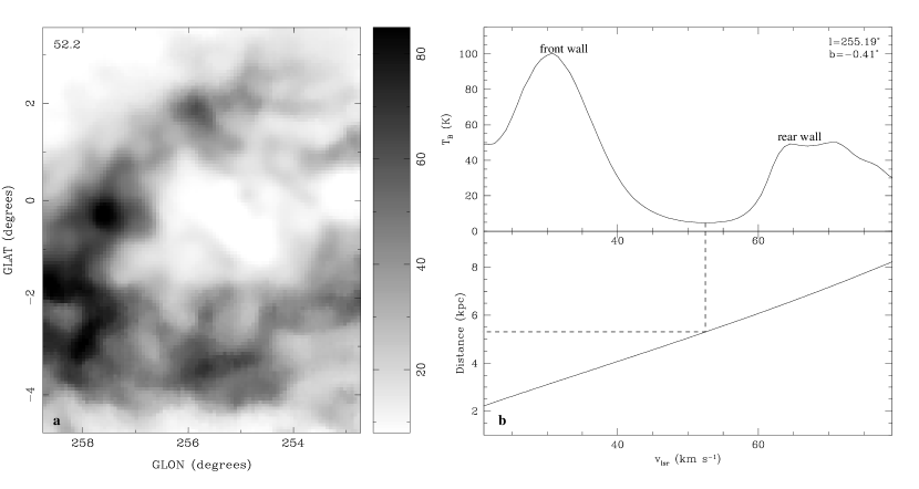
Figure 1: Grey-scale channel image of GSH 255-00+52 at $v=51.3$ ${\rm km~{}s^{-1}}$ (a) and velocity profile through the shell, with the corresponding rotation curve along the line of sight (b). The grey-scale is linear in brightness temperature as shown on the wedge at the right. The central velocity of the shell is marked with dashed lines that show the corresponding distance.

The SGPS shell catalog contains 19 new shells, four of which have been described elsewhere (McClure-Griffiths et al., 2000, 2001a). For each shell we list in Table 1 the observed parameters: center position, angular size, and expansion velocity. We define the center of the shell in galactic longitude, latitude, and velocity to be the point of minimum brightness temperature nearest to the apparent geometric center. Images of the shells and their velocity profiles are shown in Figures 1 to 15.

The expansion velocity is estimated as half of the total velocity width of the shell. This is most easily determined from the velocity profile through the center of the shell. Using the peaks on either side of the shell bowl, we determine a full velocity width for each shell. Distinguishing the fraction of a shell’s velocity width that is due to expansion from that due the spatial extent of the shell is difficult. For each shell we calculate the velocity gradient along the line of sight and compare the observed velocity width of the shell to the inferred velocity width due to the spatial extent of the shell. In order to do this we assume that the shell is nearly spherical and then calculate the expected velocity width from the velocity gradient. In all cases the velocity spread due only to the spatial extent of the shell is less than 20% of the observed shell velocity width. We therefore assume that the observed width is due to expansion and estimate that, to first order, the expansion velocity is half of the full velocity width, $v_{\rm exp}\approx\Delta v/2$.

Kinematic distances and physical sizes are determined from the shell’s center velocity, using the rotation curve of Fich, Blitz, & Stark (1989), and the angular diameters of the major and minor axes of the shell. We adopt the IAU standard values for the Sun’s orbital velocity, $\Theta_{\rm o}=220$ ${\rm km~{}s^{-1}}$ and Galactic center distance, $R_{\rm o}=8.5$ kpc. Error estimates for distance determinations assume that the dominant cause of departures from Galactic circular rotation is streaming motions, which can be as high as $\sim 10$ ${\rm km~{}s^{-1}}$ (Burton, 1988).

The mass swept-up by the expanding shell is calculated from the column density through the center of the shell, including all gas associated with the feature. We assume that the column density in the void is negligible and calculate the mass from the mean column density near the center of the shell. The error in this calculation is based on the standard deviation of the mean. We assume that most of the mass in the near and far shell walls, or “caps,” has been swept-up from the shell interior. The column density can then be used to estimate the ambient density of the medium into which the shell expanded. We assume a spherical geometry and use the axis in the plane as the characteristic radius because the assumption of a constant ambient density along the plane is more reasonable than perpendicular to the plane, where the density will drop off with latitude. Finally, the swept-up mass is calculated from the shell volume and ambient gas density. The errors in column density and those in radius propagate through to the ambient density and swept-up mass.

H i shell energetics are often characterized by the expansion energy, $E_{E}$, which is defined by Heiles (1984) to be the equivalent energy that would have to be instantaneously deposited at the shell center to account for the shell’s radius, $R_{\rm sh}$, and current rate of expansion, $v_{\rm exp}$. We give this energy as an alternative to the shell kinetic energy, as derived by McCray & Kafatos (1987), because it accounts for energy losses due to radiative cooling. Based on the Chevalier (1974) calculations for supernova remnant expansion, the expansion energy is given by $E_{E}=5.3\times 10^{43}\,n_{\rm 0}^{1.12}\,R_{\rm sh}^{3.12}\,v_{\rm exp}^{1.4}$ ergs, where $R_{sh}$ is in units of pc, $v_{exp}$ is in ${\rm km~{}s^{-1}}$, and $n_{0}$ is in ${\rm cm^{-3}}$ (Heiles, 1984). The expansion energy is strongly dependent on the shell radius and for a large shell with a non-zero expansion velocity, the required formation energies can be very large, $\sim 10^{53}$ ergs.

The ages of shells are very difficult to determine in the absence of an observed power source. As a substitute, the dynamic age, an estimate of the age based on dynamic properties, is often quoted for shells. One commonly used technique is to calculate the dynamic age from the Weaver et al. (1977) analytic solutions for a thin, expanding shell with a continuous rate of energy injection. An alternative, which we have adopted here, is to calculate the dynamic age from the equations used to describe the evolution of a supernova remnant in the late radiative phase. In the radiative phase the shock radius evolves with time as $R\propto t^{0.3}$ (Chevalier, 1974; Cioffi, McKee, & Bertschinger, 1988). So the dynamic age, $t_{6}$ in units of Myr, for a shell of radius, $R_{sh}$ given in units of pc, and expansion velocity, $v_{\rm exp}$ in units of ${\rm km~{}s^{-1}}$, is $t_{6}=0.29R_{sh}/v_{\rm exp}$. For comparison, the ages given here are a factor of $\sim 2$ less than those calculated with the Weaver et al. (1977) equations. The derived parameters: physical dimensions, expansion energy, swept-up mass, and column density are given in Table 2.

3.3 Selected Individual Shells

For some shells, the properties were either exceptional or unusually complex to calculate. Here we describe those shells, explaining how the distances and other properties were determined and in one case suggesting a possible power source. Images and detailed descriptions of GSH 277+00+36 and GSH 280+00+59, and GSH 304-00-12 and GSH 305+01-24 are given in McClure-Griffiths et al. (2000) and McClure-Griffiths et al. (2001a), respectively. The remaining shells are best demonstrated by the images and velocity profiles shown in Figures 1 to 15.

3.3.1 GSH 267-01+77

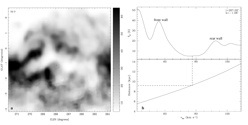
Figure 4: Grey-scale channel image of GSH 267-01+77 at $v=77.7$ ${\rm km~{}s^{-1}}$ (a) and velocity profile through the shell, with the corresponding rotation curve along the line of sight (b). The grey-scale is linear in brightness temperature, as shown on the wedge at the right. The central velocity of the shell is marked with dashed lines that show the corresponding distance.

As seen in Figure 4, the morphology of GSH 267-01+77 is irregular. The shell changes shape dramatically with velocity, but maintains a very strongly emitting rim around the H i void. It is likely that this shell was formed by the merger of several spatially distinct shells. However, the velocity profile is consistent throughout the shell and has clear walls. The physical axes of the full structure are $840\times 560$ pc and the expansion velocity is 18 ${\rm km~{}s^{-1}}$, which leads to an expansion energy of $1.8\times 10^{53}$ ergs. It is perhaps more reasonable to consider the structure as three individual shells with radii on the order of 100 pc and expansion energies on the order of $\mbox{few}\times 10^{51}$ ergs. Because the expansion energy goes as $R_{sh}^{3.14}$, considering the system as three shells each of radius $R_{sh}=R_{\rm tot}/3$, the expansion energy for the system, $E_{E}=E_{1}+E_{2}+E_{3}$, is decreased by a factor of $\sim 10$. This seems to eliminate the need for populous OB associations at large galactocentric radii (GSH 267-01+77 is at $R_{G}=12.9$ kpc) by reducing the required number of supernovae and/or massive stellar winds from $\sim 180$ to $\sim 18$.

3.3.2 GSH 297-00+73

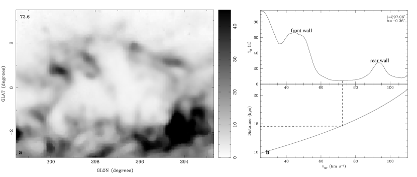
Figure 8: Grey-scale channel image of GSH 297-00+73 at $v=73.6$ ${\rm km~{}s^{-1}}$ (a) and velocity profile through the shell, with the corresponding rotation curve along the line of sight (b). The grey-scale is linear in brightness temperature, as shown on the wedge at the right. The central velocity of the shell is marked with dashed lines that show the corresponding distance.

GSH 297-00+73, shown in Figure 8, also appears to be a composite shell. There is a narrow wall separating two original shells at $l=297\fdg 2$. The wall is particularly strong near $v=63$ ${\rm km~{}s^{-1}}$ and $v=92$ ${\rm km~{}s^{-1}}$. As seen in Figure 8, the wall disappears almost completely near the center velocity of the composite structure. The decrease in emission may be due to an increased level of ionization from the merger. If we interpret the composite structure as two merged shells, one shell of $R_{1}=390$ pc, $v_{\rm exp1}=23$ ${\rm km~{}s^{-1}}$ and another of $R_{2}=315$ pc, $v_{\rm exp2}=20$ ${\rm km~{}s^{-1}}$, then the total expansion energy is $E_{E}=E_{1}+E_{2}=1.9\times 10^{53}$ ergs. This shell is far away from any other evidence of star formation, there are no H ii regions nearby nor any other tracers of spiral arms.

3.3.3 GSH 298-01+35

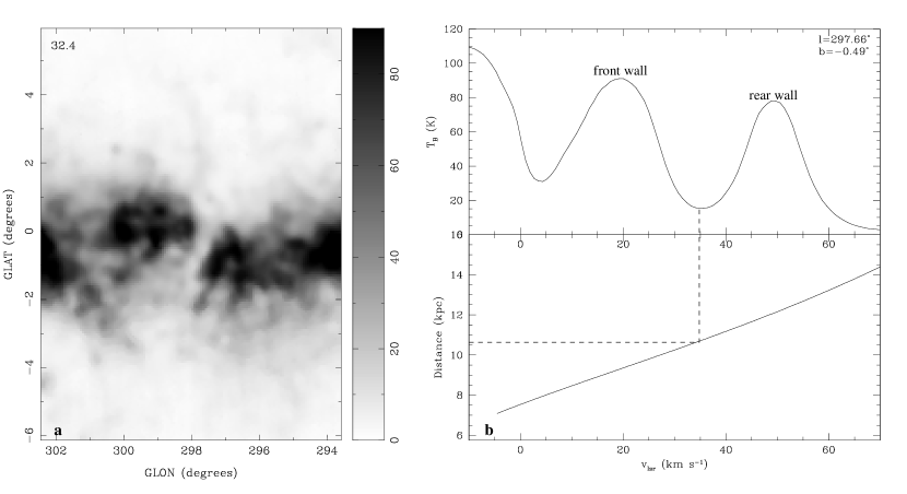
Figure 9: Grey-scale channel image of GSH 298-01+35 at $v=32.4$ ${\rm km~{}s^{-1}}$ (a) and velocity profile through the shell, with the corresponding rotation curve along the line of sight (b). The grey-scale is linear in brightness temperature, as shown on the wedge at the right. The central velocity of the shell is marked with dashed lines that show the corresponding distance.

Figure 9 shows GSH 298-01+35, a unique chimney or “worm.” The structure is very narrow in the longitudinal direction, but extends several degrees out of the plane. The chimney cuts through the Galactic plane at a slight angle and then opens above and below the plane. There is no evidence for closure within 6 degrees of the Galactic plane. The kinematic distance is $10.5$ kpc, which places it near the edge of the Sagittarius-Carina spiral arm. At this distance the chimney is only 75 pc across but extends more than a kiloparsec above the plane. The conditions required to confine a shell so dramatically along the plane and still allow for expansion into the halo are unclear. The shell also has an unusual velocity profile, in which the bowl is not very deep.

We have estimated the energy required to create a spherical cavity of radius 75 pc with an expansion velocity of 10 ${\rm km~{}s^{-1}}$ as $\sim 1.1\times 10^{52}$ ergs. We add the caveat that this may be a severe underestimate if the shell has been significantly confined along the plane. Near this position and velocity, between $v=+16$ ${\rm km~{}s^{-1}}$ and $v=+31$ ${\rm km~{}s^{-1}}$, are several H ii regions cataloged by Caswell & Haynes (1987). The closest H ii region, G298.22-0.33, is at $v=+31$ ${\rm km~{}s^{-1}}$ placing it near the center of the chimney.

3.3.4 GSH 337+00–05

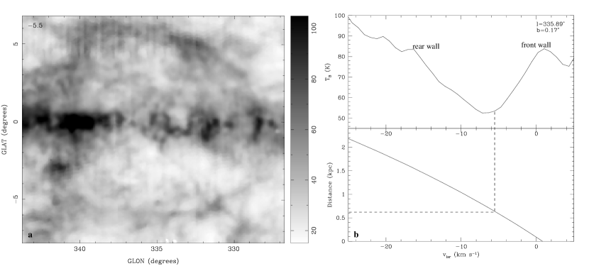
Figure 13: Grey-scale channel image of GSH 337+00–05 at $v=-5.5$ ${\rm km~{}s^{-1}}$ (a) and velocity profile through the shell, with the corresponding rotation curve along the line of sight (b). The grey-scale is linear in brightness temperature, as shown on the wedge at the right. The central velocity of the shell is marked with dashed lines that show the corresponding distance.

Figure 13 is an image of the very large angular diameter shell, GSH 337+00–05. The shell has a very thin rim and regular elliptical shape. The H i void is bisected by emission from the Galactic Plane. Kinematic distances for GSH 337+00–05 are 570 pc or 15 kpc. The small radial velocity, however, makes these distances quite uncertain. At the near distance the shell has a size of $185\times 125$ pc, whereas at the far distance it would have a diameter of nearly 4 kpc. Such a large diameter is unlikely, therefore we place the shell at $\sim 570$ pc, on the near edge of the Sagittarius-Carina arm. Because of the shell’s very local systemic velocity, it is difficult to determine the expansion velocity. The local gas is largely filled, so the emission profile bowl (shown in Fig. 13) is not well-defined. However, from the profile we find an expansion velocity of 9 ${\rm km~{}s^{-1}}$ with some uncertainty. We assume an ambient density of $1~{}{\rm cm^{-3}}$ and calculate a swept-up mass of $1\times 10^{5}~{}{\rm M_{\sun}}$. From the radius and expansion velocity an expansion energy of $1.6\times 10^{51}$ ergs is calculated.

The shell may be correlated with Ara OB1a, an association of 14 O, B, and A stars at an adopted distance of 1.38 kpc. The stars are distributed between $l=335\arcdeg$ to $l=341\arcdeg$ and $b=\pm 3\arcdeg$, which places them in the boundaries of shell. Distance moduli for the individual stars indicate distances between 790 and 2125 pc, with a mean distance of $1460\pm 125$ pc. Additionally, stars with measured radial velocities are between $-20$ ${\rm km~{}s^{-1}}$ and $+5$ ${\rm km~{}s^{-1}}$, which agrees with the central velocity of the shell. These coincidences suggest that the cluster and shell are related. If we assume that the association has 14 stars each with a representative stellar wind luminosity of $L_{w}\sim 6\times 10^{35}~{}{\rm ergs~{}s^{-1}}$, corresponding to that of a B0 star, we find that the expansion energy of the shell is consistent with formation by this cluster with an age of $\sim 6$ Myr. Because of large uncertainties in the kinematic distance of the H i shell are larger than the distance itself ($D=570\pm 900$ pc) a definitive identification is not possible.

3.4 Selection Biases

Identifying shells by eye is a subjective process and results in a number of biases in the compiled catalog. The stringent selection criteria used in this paper differ from those used for the Heiles (1979, 1984) catalogs. These criteria severely limit the number of shells included in the catalog, but the confidence level of the classification is high. There remain many shell-like structures that do not meet all criteria and were therefore not included in the catalog. Because the structure of the H i in the outer Galaxy can be characterized as largely filamentary, it is impossible to estimate the number of arched filaments that may be shells. Hence this catalog significantly underestimates the number of shells, perhaps by a factor or three or more. Comparison with the surveys of the Large and Small Magellanic Clouds (Kim, 1998; Stanimirović et al., 1999), for example, would lead us to expect the identification of many more shells.

The number of H i shells from this catalog found in the outer Galaxy outnumbers those in the inner Galaxy by almost a factor of four. This occurs for a number of reasons. Firstly, shells in the outer Galaxy are considerably easier to detect than those in the inner Galaxy. The distance ambiguity results in a much higher filling factor for H i emission at all inner Galaxy velocities. Objects that might otherwise appear as voids are filled by emission from another Galactic position. This selection bias is exacerbated by the criterion that shells exhibit a characteristic bowl in the velocity profile; candidate shells in the inner Galaxy often do not have such a well defined dip in the velocity profile. Secondly, the limited latitude coverage of the survey restricts the number of nearby shells detected. The cubes used to identify shells cover $16\arcdeg\times 22\arcdeg$ each. Extremely large ($\gtrsim 10\arcdeg$) angular diameter shells may extend beyond the edge of the cubes and are therefore difficult to find. The two extremely large angular diameter shells included in the catalog, GSH 304-00-12 and GSH 337+00-05, are unusually continuous and straightforward to detect. Because longitudes towards the third quadrant ($l<310\arcdeg$) cover more of the outer Galaxy at comparatively nearby distances, more shells can be detected. Lines of sight at high longitudes ($l>340\arcdeg$) cross large distances interior to the solar circle before reaching the outer Galaxy. As a result, outer Galaxy shells at these longitudes are very distant and therefore difficult to detect because of their small angular sizes and weak emission.

It is difficult to overcome selection biases in H i shell catalogs. An obvious solution would be to employ an automated searching algorithm. Several attempts have been made to create automated searching routines for H i shell identification (e.g. Thilker et al., 1998). The Thilker et al. (1998) technique is based on a three-dimensional cross correlation between a simulated pattern and real data. While this technique seems to be effective in external galaxies, attempts to apply the technique to the Milky Way have have not been very successful at detecting large shells. The complicated rotation curve, coupled with the fact that shells are typically non-spherical and intertwined, makes it difficult to apply an automated technique. Mashchenko et al. (1999) have extended the three-dimensional hydrodynamical simulations of shells to include more realistic models. This technique has been applied with moderate success in Canadian Galactic Plane Survey (CGPS) data (Mashchenko et al., 1999). However, the application has been limited to shells around single stars for which the physics is more straightforward than for supershells.

4 Spatial Distribution of H i Shells

One objective of the SGPS shell catalog is to explore the Galactic distribution of shells and determine how their properties vary with Galactic position. To this end, we have examined an azimuthally averaged sample of H i shell size versus Galactic radius. It has long been noticed in external galaxies, as well as in the Milky Way, that the largest H i shells are also at large galactocentric radii (e.g. Heiles, 1979; Deul & den Hartog, 1990; Walter & Brinks, 1999; Crosthwaite, Turner, & Ho, 2000). Walter & Brinks (1999) noted that in other galaxies, where there are no distance ambiguities that plague distribution studies of the Milky Way, most large shells are at galactocentric radii of more than 50% of the exponential scale length of the disk. Using shells from the SGPS and Heiles (1979, 1984) we plot the shell radius as a function of galactocentric radius in Fig. 16. Clearly, the largest shells are also at large Galactic radii. As mentioned in §3.4, Galactic H i shell catalogs exhibit a bias towards outer Galaxy shells. However, the identification of the same trend in external galaxies is convincing evidence that the observed effect is real.

A commonly suggested cause of this effect is the increase in the scale height of the H i disk with galactocentric radius(Bruhweiler et al., 1980). Shell size is intimately connected with the H i scale height; as long as a shell is smaller than the scale height it can expand three-dimensionally. However, once a shell’s size exceeds the scale height expansion in the plane is largely halted as the shell expands rapidly towards the halo and eventually bursts, venting its hot interior gas to the halo (Mac Low et al., 1989). The correlation between maximum shell size and H i scale height is best exemplified in dwarf galaxies, such as IC 2574 and Holmberg II, which have H i disk scale heights of 350-400 and 625 pc respectively and where H i shells are observed with diameters in excess of 1 kpc (Walter & Brinks, 1999; Puche et al., 1992). In gas-rich spirals, like M31, M33, and the Milky Way, flaring of the H i disk may allow shells at outer radii to reach very large sizes while shells at inner radii are confined. Other causes have been suggested to explain why the largest shells are at large galactic radii. For instance, two-dimensional hydrodynamical simulations by Wada & Norman (1999) show that H i cavities in the outer disk grow larger than those in the inner disk because of the disruptive effects of supernovae on the creation of large-scale structures in the inner disk. Below we suggest another possible effect.

The number of large H i shells beyond the solar circle seems to present a challenge to the theory of shell formation from stellar winds and supernovae. Assuming that the energy output of a single O or B type star is $\sim 10^{51}$ ergs, associations of several hundred massive stars are needed to create expanding shells with radii of a few hundred parsecs. It is difficult to understand how the star formation rates in the outer Galaxy can be high enough to account for the many large shells. For example, in the small SGPS sample there are five shells in the region $267\arcdeg\leq l\leq 297\arcdeg$, $10.0\leq R_{gal}\leq 13.3$ kpc with expansion energies in the range $1.8-2.4\times 10^{53}$ ergs. That implies a shell surface density of $\sim 0.3~{}{\rm kpc^{-2}}$, with each shell requiring more than 150 supernova progenitors to form. We can compare the observed surface density with the McKee & Williams (1997) predictions for the surface density of clusters with $\mathcal{N}_{\ast h}$ supernova progenitors, as a function of Galactic radius. Using their equation (44), scaled to a mean galactocentric radius of 11 kpc, we find that for $\mathcal{N}_{\ast h}=150$ the predicted surface density of clusters is also $\sim 0.3~{}{\rm kpc^{-2}}$. Despite this very good agreement we note that the SGPS catalog is not complete. The Heiles (1984) catalog has a much higher surface density of energetic shells, which cannot be accounted for by the McKee & Williams (1997) star formation rate. In addition, though the functional form of cluster surface density allows for populous OB associations at large galactocentric radii, there is no evidence for any current giant H ii regions beyond 11 kpc (McKee & Williams, 1997; Smith, Biermann, & Mezger, 1978). Barring a dramatic change in the star formation history of the outer Galaxy sometime in the last $\sim 20$ Myr, there seems to be a discrepancy between the observed giant H ii regions and H i supershells. We are left, therefore, with a population of energetic shells in the outer Galaxy that cannot be adequately accounted for by the observed star formation rate.

Attempting to resolve this discrepancy, we consider the possibility that the expansion energies have been over-estimated. In particular we explore the relationship of shell size and expansion energy to the ambient density into which the shells expand. If the ambient densities are lower in the outer Galaxy, as was found around several shells in our catalog, then shells there should reach larger sizes than those in the inner Galaxy. Referring to the expansion energy equation given above, for a fixed input energy and expansion velocity, the shell radius varies with ambient density, $n_{0}$, as $R_{sh}\propto n_{0}^{-0.36}$. Unfortunately, this is not a strong dependency and H i densities do not vary by more than a factor of 3 to 4 across the disk (Burton, 1988). It is unlikely, then, that shells in the outer Galaxy grow larger than those in the inner Galaxy by more than a factor of $\sim 1.7$ (for a density decrease of a factor of 4) due to external density variation alone. This does not seem to be a large enough effect to explain the distribution shown in Fig. 16. Similarly, the calculated expansion energy is only weekly dependent on the ambient density, $n_{0}$, such that $E_{E}\propto n_{0}^{1.12}$ so that ambient density alone cannot account for the highly energetic shells at large Galactocentric radii. However, Walter & Brinks (1999) point out that the constant in the expansion energy equation ($5.3\times 10^{43}$ in the energy equation given in §3.2) is dependent on cooling rates and includes an assumption about elemental abundances. Elemental abundances are not constant throughout the Galaxy and are thought to decrease by more than an order of magnitude with Galactic radius (Shaver et al., 1983). Because metals are efficient at cooling, a high metallicity environment requires more energy for a shell to attain a given radius. Therefore, for shells in the outer Galaxy where the metallicities are lower, the expansion energies may be slightly over-estimated.

One can also use a simple timescale argument to explain the observation that the largest H i shells are found at large Galactic radii. The frequency with which a spiral density wave encounters matter in a differentially rotating disk, expressed in units of $\kappa$, the epicyclic frequency, is $\nu^{2}=m^{2}(\Omega_{p}-\Omega)^{2}/\kappa^{2}$, where $m$ is the number of spiral arms, $\Omega_{p}$ is the angular velocity of the spiral pattern, and $\Omega$ is the angular velocity of the gas in the disk. From the shape of the spiral arms, the spiral pattern speed is estimated to be in the range $10$ ${\rm km~{}s^{-1}}$ $\leq\Omega_{p}\leq 20$ ${\rm km~{}s^{-1}~{}kpc^{-1}}$ (e.g. Lépine et al., 2001; Amaral & Lèpine, 1997). Therefore at a Galactocentric radius of $\sim 9$ kpc, the gas and pattern speeds are matched. Interior to this corotation radius, $R_{CR}$, the arms move more slowly than the gas, resulting in a spiral shock on the counter-clockwise side of the arms (as seen from the North Galactic Pole), or the side towards the Galactic center. Star formation occurs near this shock and we would expect small H i shells to form here. Exterior to the corotation radius the arms move faster than the disk gas, hence the spiral shock is on the exterior edge of the arms. At a galactic radius of 8 kpc, the spiral arms travel with a linear velocity, $v=\Omega_{p}R_{gal}\approx 120$ ${\rm km~{}s^{-1}}$(assuming $\Omega_{p}\sim 15~{}{\rm km~{}s^{-1}~{}kpc^{-1}}$). At the same distance, however, the gas in the disk rotates with a velocity of $220$ ${\rm km~{}s^{-1}}$. For an arm width of 3 kpc, the gas crosses the arm in $\sim 30$ Myr, which is comparable to the formation timescale for a large H i shell (Oey & Clarke, 1997). Therefore, if the first wave of star formation occurs on the leading edge of the spiral arm then we might expect to see small H i shells formed from several stars located there. As the density wave passes through the disk, triggering more star formation, an H i shell can carve out a progressively larger and larger volume of the ISM. This is accompanied by the movement of the spiral arm such that by the time a large shell has been created, the gas will have moved away from the spiral arm.

By contrast, at a Galactic radius of 3 kpc, the arms only move at $\sim 45$ ${\rm km~{}s^{-1}}$, whereas the gas still travels at $220$ ${\rm km~{}s^{-1}}$. In this case, the gas crosses a 3 kpc spiral arm in less than $\sim 17$ Myr, but more importantly, it also crosses the interarm region in a comparable amount of time. Therefore, a shell at a Galactic radius of $<5$ kpc, which is formed in a spiral arm will move out of the arm, through the interarm region, and encounter the next arm before it reaches its maximum radius. The encounter with the next spiral shock should be enough to completely disrupt the shell. This, along with the flaring of the outer H i disk, may explain why large shells are only seen in the outer Galaxy. At small Galactic radii they do not survive long enough to reach a large size.

4.1 Shells and Spiral Structure

We can also use the shell catalog to examine how H i shells are spatially related to Galactic spiral structure. Thilker (1999) found a strong correlation between spiral arms and H i shells in NGC 2403, M81 and M101. In these galaxies many shells are located between the spiral arms, usually extending from the arms into the interarm regions. Deul & den Hartog (1990) noted the presence of large H i holes in interarm regions of M33. NGC 4214 has three large shells between the spiral arms and no detectable shells in the arms (Walter et al., 2001). Similarly, some of the SGPS shells extend into interarm regions; GSH 277+00+36 and GSH 280+00+59 are particularly clear examples (McClure-Griffiths et al., 2000). A comparison of our shells with the Milky Way spiral arms is important. Unfortunately, spiral structure in the Milky Way is poorly understood. Our unique position within the Galaxy makes tracing the spiral structure particularly difficult. The number of spiral arms, placement of the arms and even the H i response to the spiral arms are all largely unknown. One major obstacle is the necessity of a well understood rotation curve to calculate kinematic distances. The Milky Way rotation curve is uncertain, as are the precise effects of streaming motions. Molecular line emission and H ii regions are often used as tracers of spiral structure, but many interpretations of these also rely on kinematic distances.

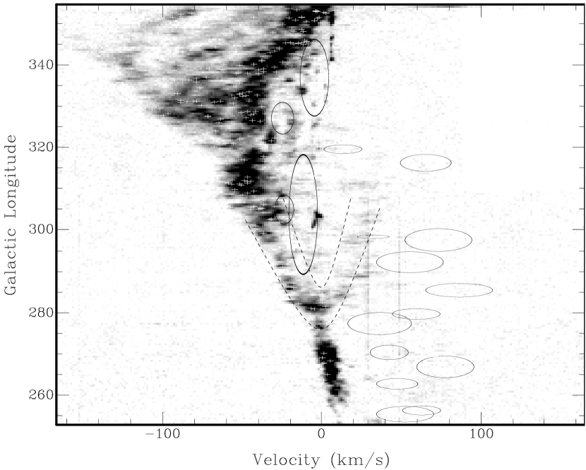
Figure 17: SGPS H i shells plotted on the ¹²CO l-v image from Dame et al. (1987). The ellipses mark the SGPS shells and the white crosses mark H ii regions cataloged by Caswell & Haynes (1987) on the basis of their recombination lines. The dashed lines outline the “Carina Loop,” part of the Sagittarius-Carina arm

In order to eliminate the rotation curve dependence it is often preferable to address Galactic distributions with respect to the longitude-velocity (l-v) distribution, which does not include any assumptions about distance. In Fig. 17 we have plotted the SGPS shells on the ¹²CO l-v diagram from Dame et al. (1987). The CO emission has been averaged for latitudes over the range $|b|<2\arcdeg$. Also included on this figure are H ii regions from Caswell & Haynes (1987) marked with white crosses. The shells, marked by ellipses, are located at their cataloged positions and their plotted sizes are determined by their angular diameters and velocity widths. Over the range $v=-100$ ${\rm km~{}s^{-1}}$ to $v=0$ ${\rm km~{}s^{-1}}$ and $l>310\arcdeg$ the velocity structure is complicated and consequently the individual spiral arms are unclear. The only spiral feature that is immediately distinguishable is the Carina Loop, part of the Sagittarius-Carina arm near $l=280\arcdeg$, marked with dashed lines on Fig. 17. Few shells are coincident with the spiral tracers, instead most lie in regions not associated with spiral structure. The small chimney-like structure, GSH 298-01+32, is embedded in the edge of this spiral arm, apparently containing, or perhaps even the result of, an H ii region. Outside of the loop, towards more positive velocities the shells GSH 277+00+36, GSH 280+00+59, GSH 292-01+55, and GSH 297-00+72 seem to trace the arc of the loop. Another interesting feature is the placement of GSH 304-00-12 (large ellipse at the center of Fig. 17) in an interarm region and bounded by CO emission from the Coalsack nebula near $v=0$ ${\rm km~{}s^{-1}}$.

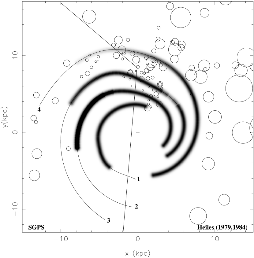
Figure 18: Cataloged shells plotted on the spiral pattern of the Galaxy from Taylor & Cordes (1993). As marked, shells in the first and second quadrant are from Heiles (1984) and shells in the fourth quadrant are from this work. The spiral arms are labelled 1-4 according to the following 1: Norma, 2: Scutum-Crux, 3: Sagittarius-Carina, and 4: Perseus. The Galactic center is marked by a cross-hair and the position of the Sun is marked by circle with a dot at the center. The SGPS survey region is marked by straight, solid lines.

To expand the distribution study to more global scales, we have included the shells with $|b|<5\arcdeg$ from Heiles (1979, 1984). Figure 18 is a diagram of H i shells from the SGPS and Heiles (1979, 1984) catalogs plotted on the spiral arms of the Galaxy as defined in the Taylor & Cordes (1993) electron density model. The Taylor & Cordes (1993) model fits the arms on the basis of the Georgelin & Georgelin (1976) spiral model from H ii regions and radio-continuum features that mark the spiral arm tangents. The model describes the electron density distribution of the Galaxy, which is very much related to star formation, and is the most detailed model of the spiral arm positions available. The arms given by Taylor & Cordes (1993) have been extended (narrow lines on Fig. 18) to approximate a spiral pattern. It should be stressed that the extensions are extrapolations and are not based on spiral tracers. Shell positions are also uncertain. Departures from circular rotation caused either by the underlying spiral pattern or other systemic effects are not accounted for in their positions. These departures can be as high as $\sim 10$ ${\rm km~{}s^{-1}}$, and therefore the positions of all shells are uncertain at the 5-20% level. The Heiles (1979, 1984) shells are on the right-hand side of the figure and the shells on the left are from the SGPS. Many of the large cluster of local shells from the Heiles (1979, 1984) catalog seem to lie between the Sagittarius-Carina arm and the Perseus arm. Among the SGPS shells, some are clearly located between the spiral arms. The extreme distance of several of the shells, however, makes it difficult to compare them to the spiral arms because they are beyond the known extent of the arms.

Figs. 17 & 18 seem to suggest that an appreciable number of H i shells overlap interarm regions. The most convincing examples of interarm shells are the outer Galaxy chimneys, GSH 277+0+36 and GSH 280+0+59, and the Coalsack shells, GSH 305+01-24 and GSH 304+00-12, which are all found on the edge of the Sagittarius-Carina spiral arm and open into the region between the Sagittarius-Carina and Perseus arms. Because only a portion of one spiral arm is clear in the l-v diagram and the distribution of shells from a face-on view of the Galaxy is subject to distance determination uncertainties, it is not possible to determine how strongly the correlation holds. We note that the distribution could be partially a selection effect; H i shells at the edge of spiral arms are easier to detect than those in arms. Certainly there are enough shells between spiral arms to raise the question, why are they there?

While we expect star formation to occur in the spiral arms, the $\sim 30$ Myr required to form a large shell is long enough that shells may migrate out of the spiral arms into interarm regions. So, this distribution is not surprising. Another important component to the shell distribution may be the density structure of the Galactic disk, in particular the density gradient at the transition from spiral arm to interarm region. At this transition the density gradient may lead to enhanced expansion of the shell. Unlike the leading edge of the arm, the gravitational potential well at the back side of the arm is not very steep and there are no shocks to disturb the shell’s expansion. As a result, the shell may largely escape the spiral arm and expand along the density gradient into the interarm region. The result could be inordinately large shells in interarm regions.

4.1.1 Simple Spiral Structure Model

To explore this theory we need to know the strength of the density gradient, which can be naively estimated from a simple spiral perturbation model of the disk. Following the arguments of Roberts & Hausman (1984, hereafter RH84), they define the two-dimensional, spirally perturbed disk gravitational potential as

$$U(r,\theta,t)=U_{0}(r)\left\{1+\xi(r)\cos\left[m\theta-m\Omega_{p}t+\Phi(r)\right]\right\},$$ (1)

where $r$ is the galactocentric radius, $\theta$ is the azimuthal angle, $U_{0}$ is the unperturbed potential, $\Omega_{p}$ is the pattern speed, and $\xi$ and $\Phi$ are the amplitude and phase, respectively, of the spiral perturbation. The unperturbed potential, $U_{0}$, is that of a Toomre disk (Toomre, 1963) given by

$$U_{0}\left(r\right)=-\frac{B^{2}a^{3}}{\left(a^{2}+r^{2}\right)^{1/2}},$$ (2)

where the constants $a=7$ kpc and $B=0.0576~{}{\rm Myr^{-1}}$ have been chosen to give a peak circular velocity of 220 ${\rm km~{}s^{-1}}$ at 8.5 kpc. The amplitude of the spiral perturbation is,

$$\xi(r)=\frac{A}{5}\,\frac{a^{2}r^{2}}{\left(a^{2}+r^{2}\right)^{2}}.$$ (3)

The constant, $A=0.067$, was chosen to make a spiral perturbing force that is $5-10$% of the unperturbed force. The phase of perturbation is given by

$$\Phi(r)=\frac{2\ln\left[1+\left(r/r_{0}\right)^{j}\right]}{j\tan i_{0}},$$ (4)

where $i_{0}$ is the pitch angle of the spiral, set to 10° in RH84. The phase is defined to make a transition between a bar-like potential at $r<r_{0}=1$ kpc and a spiral-like potential at $r>r_{0}$. The power $j=5$ determines how sharply this transition takes place.

We are concerned with the surface density response to the gravitational potential. Therefore Poisson’s equation must be solved for the surface density from the Toomre and spiral potentials. Given the unperturbed potential in equation 2, the unperturbed surface density from RH84 is:

$$\sigma_{o}\left(r\right)=\frac{B^{2}a^{4}}{2\pi G\left(a^{2}+r^{2}\right)^{3/2}}.$$ (5)

Following Lin et al. (1969) and Freeman (1975) we solve Poisson’s equation with the spiral potential for the linear density response of the total gas and stars, by making an asymptotic approximation that the pitch angle is small and therefore the quantity $[\Phi^{\prime}(r)r]^{-1}$ is small. The total surface density perturbation (gas and stars) is then given by:

$$\sigma_{p}=\frac{U_{o}(r)\xi(r)}{2\pi G}\Phi^{\prime}(r)\cos[m\theta-m\Omega_{p}t+\Phi(r)],$$ (6)

where $m$ is the number of arms. The total surface density, including the Toomre disk, is simply $\sigma_{t}=\sigma_{o}(r)+\sigma_{p}(r)$. Using the two-dimensional surface density given by these equations we modified the original RH84 parameters to better fit the Georgelin & Georgelin (1976) and Taylor & Cordes (1993) model for the spiral arms. Rather than assuming a two-armed spiral we used a four-arm spiral with a pitch angle of $11\fdg 5$ and decreased the amplitude of the spiral perturbations so that $A=0.05$. We found that these modifications gave a better fit to the Taylor & Cordes (1993) model for the spiral pattern and agree well with recent work by Vallée (2002). We note, though, that the model employed here is not designed to perfectly fit the observed Milky Way, but rather given what we do know about the spiral structure near to the Sun, to estimate the relative magnitudes of the $z$ and $r$ components of the density gradient.

The question of how the H i reacts to the spiral potential is non-trivial. The density derived in equation 6 neglects the effects of star formation, which through photo-dissociation may be significant in minimizing the arm-interarm density contrasts in H i. In addition, while the stellar disk dominates the mass density at small galactic radii, the gas disk dominates over the stellar disk for large radii. We have therefore modified the surface density to reflect the smaller arm-interarm contrasts seen in the Galaxy (Burton, 1988) and to decrease the axisymmetric drop in density. We relate the surface density to the volume density at midplane according to $\Sigma_{HI}=\sqrt{2\pi}\sigma_{z}\rho_{HI}(0)$, where $\sigma_{z}=120$ pc (Dickey & Lockman, 1990). Finally, the parameters have been adjusted to give a fiducial density of $n_{HI}\approx 0.3~{}{\rm cm^{-3}}$ at the position of the Sun.

4.1.2 Comparison of the Density Gradient

As suggested above, the ambient medium has an effect on the radius and energetics of a supershell. It has been shown that a shell expanding in a stratified medium, i.e. from the Galactic disk into the halo, will experience exaggerated expansion along the density gradient, forming a chimney (e.g. Mac Low & McCray, 1988). Though magnetic fields in the plane can confine a shell for $\sim 20$ Myr (Tomisaka, 1998), models show that the effect of the density gradient will be enough for a large shell to eventually blow out of the plane. We hypothesize that if the density gradient from arm to interarm regions is strong enough the same effect can form an in-plane chimney. We therefore need to understand the density gradient around spiral arms in order to assess the effect of the spiral arms and interarm regions on shells.

Figures 19 and 20 show radial and $z$ profiles of H i number density and density gradient. The radial profile was taken along the line-of-sight from the Sun to the Galactic center and the $z$ profile starts at mid-plane and extends to $z=200$ pc. Obviously, both models grossly oversimplify the Galactic disk, but they are instructive to show how the density varies across the disk and out of the plane. Also shown in Fig. 19 is a density gradient calculated from just the spiral perturbation to the density, but not including the underlying axisymmetric disk. This should allow for a more direct comparison of the gradient around spiral arms with that out of the plane. Comparing the two gradients, we find that for this model, at a typical height of $z=100$ pc above the mid-plane, the density gradients are of comparable magnitude. Assuming that the interstellar pressure is largely determined by the density, an expanding shell close to the Galactic plane should feel a stronger gradient away from the arm than out of the plane. Consequently the shell should expand rapidly away from the arm through the interarm medium. Towards the arm, expansion will be impeded by the higher density. As the shell continues to expand vertically it will reach a $z$-height of $\sim 100$ pc, at which point the density gradient out of the plane will begin to dominate.

4.2 Discussion

This simple model presents a possible explanation for the observation that many H i shells in the Galaxy are between the spiral arms. The combined effects of the density gradient and migration of shells may lead to a spatial offset of shells away from the spiral shock and into the interarm regions. Because shells expanding into interarm regions can reach exaggerated sizes, their formation energy requirements are reduced to levels more consistent with star formation rates. Other environmental factors that influence shell evolution may enhance the effect suggested here, namely the magnetic field and cosmic ray pressures. These may also show strong arm-interarm gradients, but it is beyond the scope of this paper to model them.

We note that the density gradient determined here depends on the number of arms and the pitch angle of the spiral. The model employed here has four arms with a relatively small pitch angle. These quantities, however, are still not well determined. We find that for a much less tightly wound spiral, with a pitch angle of $20\arcdeg$, the maximum density gradient is a factor of two less than that for a pitch angle of $11\fdg 5$. In this case, the density gradient away from spiral arms would never dominate, but is still comparable to the density gradient out of the disk. So, while the model developed in §4.1.1 was based on previous estimates of Milky Way parameters (e.g. RH84, Vallée 2002), it is sufficiently robust that its specifics can be modified and the main result, that the $z$ and $r$ components of the density gradient are of comparable magnitude, will hold. This fact should be considered when examining external galaxies in which the spiral structure may be significantly different than in the Milky Way.

A similar observation of shell-like structures at the edge of spiral arms was made by Crosthwaite et al. (2000), who came to a different conclusion. Crosthwaite et al. (2000) examined the H i in the spiral galaxy IC 342 and found several large, shell-like structures in the outer galaxy ($R>R_{CR}$). In particular, the question of whether the fine structure in the spiral arms is due to shells or flocculent arms is addressed. They determine that the holes do not have the kinematic signatures of shells, that they are not necessarily associated with star formation in the form of H$\alpha$ emission or H ii regions, that the inferred expansion energies are too large ($E_{E}\sim 3\times 10^{53}$ ergs) to be shells, and most importantly, they argue that the shells do not appear to be experiencing shearing due to differential rotation. From this last point they argue that shearing would have significantly affected their observed shells in the timescales required to create holes that large with stellar winds and supernovae. They instead explore the possibilities that the structures were formed from negative shear that created spurs on the gas arms, or alternately that the flocculent structure is due to gas instabilities that created shell-like structures and holes, similar to the instabilities suggested by Wada & Norman (1999). They determine that the surface density enhancements in the spiral arm segments are insufficient to promote negative shear and hence perpendicular arm-spurs. They therefore conclude that the data supports the hypothesis that the shell-like structures are formed from two-fluid gravitational instabilities in the gas disk, not shells. We cannot rule out that shells seen at the edges of arms in the Milky Way are also due to gravitational instabilities. However, in our limited sample of SGPS shells, the kinematic signatures are distinctly characteristic of expanding structures. Also the structure of the shell walls is consistent with shell walls formed by compression. GSH 277+00+36, for example, exhibits a very sharp shell wall and is cohesive over more than 40 ${\rm km~{}s^{-1}}$ of velocity dispersion. Both characteristics seem improbable for an object formed by gravitational instability.

The suggested scenario may explain the position and formation energy of supershell GSH 277+00+36 (McClure-Griffiths et al., 2000). In the early stages of its evolution the shell may have expanded away from the spiral arm through a region where the density steadily decreased from its central position. In this way it may have attained an exceptionally large size and therefore may not have required $10^{53}$ ergs to form. At about 100 pc, however, the gradient out of the plane would have begun to dominate and the shell expanded quickly into the halo forming a chimney. The rapid expansion and pressure differential between the halo gas and the pressurized shell interior may have resulted in Rayleigh-Taylor instabilities that formed the chimney channels seen extending from the shell to the halo. If this scenario is correct, we may see similar, though perhaps less developed, Rayleigh-Taylor instabilities developing in the walls perpendicular to the plane.

The idea that the number of large, energetic shells observed in galaxies is irreconcilable with star formation is not a new one (e.g. Rhode et al., 1999; Crosthwaite et al., 2000). Numerous alternative formation theories have been developed to overcome this “energy crisis,” including the impact of high velocity clouds (Tenorio-Tagle et al., 1987), gamma-ray bursts (Loeb & Perna, 1998), and gravitational or thermal ISM instabilities (Wada et al., 2000). Though the alternatives are appealing, and may hold true for some shells, it seems clear that we do not yet understand shells well enough to resolve the crisis. How are there so many energetic shells? Though the energy requirements can be lessened somewhat by allowing for shells expanding into interarm regions, alternative theories will have to be invoked for some shells.

5 Conclusions

We have discovered nineteen new H i shells in the Southern Galactic Plane Survey. These shells vary in radius from 40 pc to 700 pc, have expansion velocities between 6 ${\rm km~{}s^{-1}}$ and 20 ${\rm km~{}s^{-1}}$, have expansion energies between $10^{51}$ ergs and $10^{53}$ ergs and are distributed throughout the fourth quadrant of the Galaxy. We have used this new catalog, along with those of Heiles (1979, 1984), to examine the distribution of large H i shells in the Milky Way. We find a tendency for large, energetic shells to be located at large Galactocentric radii; a tendency that has also been observed in external galaxies (e.g. Deul & den Hartog, 1990; Walter & Brinks, 1999). We also show that many shells are located between the spiral arms of the Galaxy. We have used basic timescale arguments to show that the timescales are such that gas moves out of a spiral arm in a time that is comparable to the time required for the formation of a large ($R>100$ pc) shell. Hence, we believe that large shells will often end their lives between spiral arms. We have used the same timescale arguments to show that in the inner Galaxy, where few large shells are observed, a shell would move out of an arm, through the interarm region, and be struck by the next spiral arm before it could grow very large. This may explain why large shells are only seen at large Galactic radii.

We have also used spiral density wave theory to explore the radial density structure of the Galactic disk as a result of spiral arms. We compared this to the density structure extending out of the Galactic plane towards the halo to show that the density gradient away from spiral arms is comparable to that from the disk to the halo. Because simulations have shown that shells expanding out of the plane tend to elongate in that direction, we suggest an analogous scenario in which a shell experiences runaway expansion away from spiral arms. This effect, combined with the multiple generations of star formation required to create large shells, should lead to a population of interarm shells.

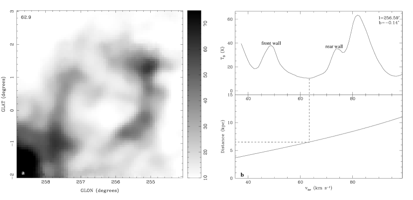
Figure 2: Grey-scale channel image of GSH 256+00+63 at $v=62.9$ ${\rm km~{}s^{-1}}$ (a) and velocity profile through the shell, with the corresponding rotation curve along the line of sight (b). The grey-scale is linear in brightness temperature, as shown on the wedge at the right. The central velocity of the shell is marked with dashed lines that show the corresponding distance.

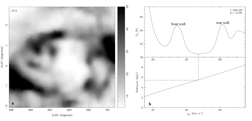
Figure 3: Grey-scale channel image of GSH 263+00+47 at $v=47.2$ ${\rm km~{}s^{-1}}$ (a) and velocity profile through the shell, with the corresponding rotation curve along the line of sight (b). The grey-scale is linear in brightness temperature, as shown on the wedge at the right.

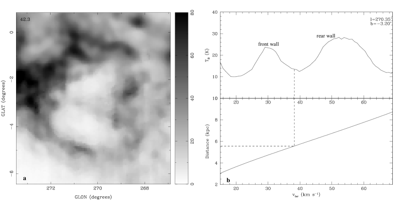
Figure 5: Grey-scale channel image of GSH 270-03+42 at $v=47.3$ ${\rm km~{}s^{-1}}$ (a) and velocity profile through the shell, with the corresponding rotation curve along the line of sight (b). The grey-scale is linear as shown on the wedge at the right. The central velocity of the shell is marked with dashed lines that show the corresponding distance.

Figure 6: Grey-scale channel image of GSH 285-02+86 at $v=86.0$ ${\rm km~{}s^{-1}}$ (a) and velocity profile through the shell, with the corresponding rotation curve along the line of sight (b). The grey-scale is linear in brightness temperature, as shown on the wedge at the right. The central velocity of the shell is marked with dashed lines that show the corresponding distance.

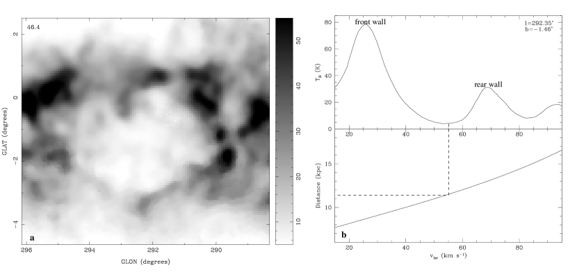
Figure 7: Grey-scale channel image of GSH 292-01+46 at $v=46.4$ ${\rm km~{}s^{-1}}$ (a) and velocity profile through the shell, with the corresponding rotation curve along the line of sight (b). The grey-scale is linear in brightness temperature, as shown on the wedge at the right. The central velocity of the shell is marked with dashed lines that show the corresponding distance.

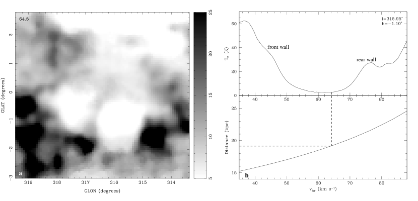
Figure 10: Grey-scale channel image of GSH 316-00+65 at $v=64.5$ ${\rm km~{}s^{-1}}$ (a) and velocity profile through the shell, with the corresponding rotation curve along the line of sight (b). The grey-scale is linear in brightness temperature, as shown on the wedge at the right. The central velocity of the shell is marked with dashed lines that show the corresponding distance.

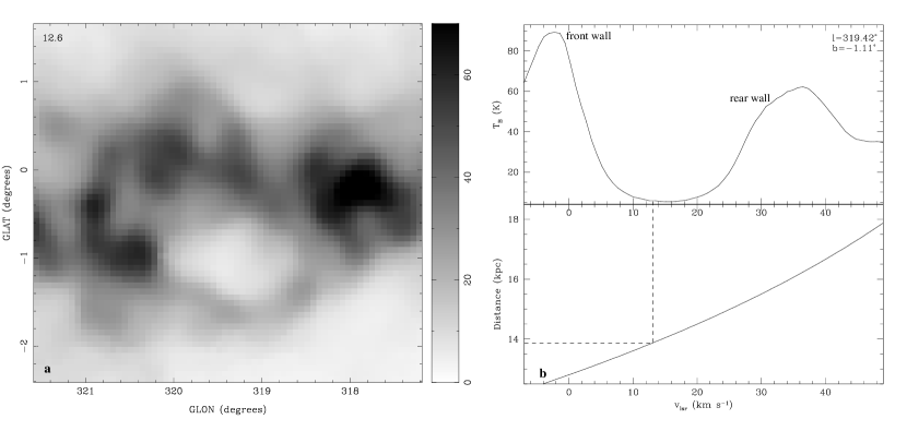
Figure 11: Grey-scale channel image of GSH 319-01+14 at $v=12.6$ ${\rm km~{}s^{-1}}$ (a) and velocity profile through the shell, with the corresponding rotation curve along the line of sight (b). The grey-scale is linear in brightness temperature, as shown on the wedge at the right. The central velocity of the shell is marked with dashed lines that show the corresponding distance.

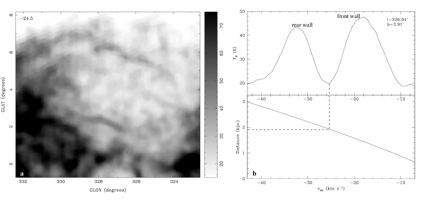
Figure 12: Grey-scale channel image of GSH 327+04-25 at $v=-24.5$ ${\rm km~{}s^{-1}}$ (a) and velocity profile through the shell, with the corresponding rotation curve along the line of sight (b). The grey-scale is linear in brightness temperature, as shown on the wedge at the right. The central velocity of the shell is marked with dashed lines that show the corresponding distance.

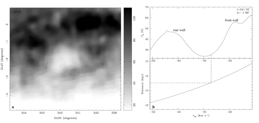
Figure 14: Grey-scale channel image of GSH 342–02–27 at $v=-27.0$ ${\rm km~{}s^{-1}}$ (a) and velocity profile through the shell, with the corresponding rotation curve along the line of sight (b). The grey-scale is linear as shown on the wedge at the right. The central velocity of the shell is marked with dashed lines that show the corresponding distance.

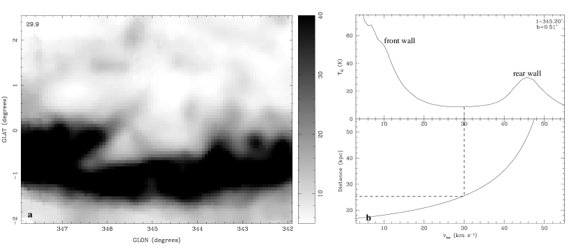
Figure 15: Grey-scale channel image of GSH 345+00+30 at $v=29.9$ ${\rm km~{}s^{-1}}$ (a) and velocity profile through the shell, with the corresponding rotation curve along the line of sight (b). The grey-scale is linear in brightness temperature, as shown on the wedge at the right. The central velocity of the shell is marked with dashed lines that show the corresponding distance.

Figure 16: Galactic H i shell radius versus galactocentric radius. All shells from the SGPS are plotted with asterisks and shells from Heiles (1979, 1984) are plotted with triangles. The general trend that large shells are found at large galactocentric radii is clear.

Figure 19: Modeled H i density and density gradient along the line of sight crossing the Sun and the Galactic center. The top panel shows the H i density profile, $n_{HI}(r)$, with a solid line. The dashed line is the one-dimensional density gradient profile, $dn_{HI}(r)/dr$, and the dotted line is the density gradient for an axisymmetric potential, not including the spiral perturbation. The scale for the volume density is at the left and the scale for the density gradient is shown on the right. The bottom panel is the residual density gradient obtained by subtracting the axisymmetric component from the total density gradient. This plot shows the effect of the spiral arms alone.

Figure 20: H i density and density gradient as a function of height above the galactic plane, $z$. The solid line is the H i number density with the axis marked to the left. The dashed line is the density gradient, $dn_{HI}/dz$, with the axis marked on the right.

Table 1: Observed properties of H i shells in the SGPS

Name	$l$	$b$	$v$	$\Delta l$	$\Delta b$	$v_{\rm exp}$	Comments
	(deg)	(deg)	(${\rm km~{}s^{-1}}$)	(deg)	(deg)	(${\rm km~{}s^{-1}}$)
GSH $255-00+52$	$255.2$	$-0.5$	$+52$	3.8	3.7	18
GSH $256+00+63$	$256.6$	$-0.1$	$+63$	2.2	2.2	12
GSH $263+00+47$	$262.9$	$-0.1$	$+47$	2.3	2.9	13	irregular shape
GSH $267-01+77$	$267.1$	$-1.1$	$+77$	5.3	3.5	18	two merged shells
GSH $270-03+42$	$270.5$	$-3.3$	$+42$	3.2	3.8	12
GSH $277+00+36$	$277.5$	$0.0$	$+36$	5.4	$>20$	20	proposed chimney
GSH $280+00+59$	$279.8$	$+0.1$	$+59$	2.6	$>20$	15	proposed chimney
GSH $285-02+86$	$285.6$	$-2.5$	$+86$	3.3	3.2	21
GSH $292-01+55$	$292.4$	$-1.5$	$+55$	5.1	2.0	21
GSH $297-00+73$	$297.2$	$-0.3$	$+73$	5.5	2.8	21	two merged shells
GSH $298-01+35$	$297.7$	$-0.5$	$+35$	0.8	$>12$	10	proposed chimney
GSH $304-00-12$	$303.9$	$-0.2$	$-12$	29	20	9	Coalsack shell
GSH $305+01-24$	$305.1$	$+1.0$	$-24$	7	$11.3$	6	assoc. w/ Cen OB1
GSH $316-00+65$	$316.4$	$-0.5$	$+65$	4.1	3.0	16	two merged shells
GSH $319-01+13$	$319.4$	$-1.1$	$+13$	2.1	1.7	18
GSH $327+04-25$	$327.2$	$+3.4$	$-25$	7.7	5.6	7
GSH $337+00-05$	$335.9$	$+0.2$	$-5$	18.6	12.5	9	assoc. w/Ara OB1a
GSH $342-02-27$	$341.8$	$-1.9$	$-27$	1.8	1.9	14
GSH $345+00+30$	$345.2$	$+0.5$	$+30$	4.7	2.5	18	unknown distance

Table 2: Derived properties for new H i shells from the SGPS

Name	$D$	$R_{gal}$	$R_{\rm major}$	$R_{\rm minor}$	$t_{D}$	$n_{0}$	$M$	$E_{E}$
	(kpc)	(kpc)	(pc)	(pc)	(Myr)	($cm^{\rm-3}$)	($10^{5}~{}{\rm M_{\odot}}$)	($10^{51}$ ergs)
GSH $255-00+52$	$5.3\pm 1.0$	$11.1\pm 0.7$	$175\pm 30$	$170\pm 30$	2.9	$1.7\pm 0.5$	$13\pm 7$	$53\pm 39$
GSH $256+00+63$	$6.5\pm 1.0$	$11.9\pm 0.8$	$145\pm 20$	$140\pm 20$	3.6	$1.0\pm 0.4$	$4.2\pm 1.9$	$9\pm 7$
GSH $263+00+47$	$5.5\pm 1.0$	$10.7\pm 0.6$	$110\pm 20$	$140\pm 25$	2.5	$1.4\pm 0.6$	$2.8\pm 1.5$	$7\pm 5$
GSH $267-01+77$	$9.2\pm 1.2$	$12.9\pm 0.9$	$420\pm 55$	$280\pm 35$	6.9	$0.4\pm 0.1$	$45\pm 17$	$177\pm 104$
GSH $270-03+42$	$6.0\pm 1.0$	$10.4\pm 0.6$	$170\pm 30$	$200\pm 30$	4.2	$0.8\pm 0.2$	$5.3\pm 2.6$	$11\pm 8$
GSH $277+00+36$	$6.5\pm 0.9$	$10.0\pm 0.5$	$305\pm 45$	$>1000$	4.5	$1.2\pm 0.1$	27-56	$240\pm 120$
GSH $280+00+59$	$9.4\pm 0.9$	$11.5\pm 0.7$	$215\pm 20$	$>1000$	4.8	$0.6\pm 0.1$	$11\pm 2$	$26\pm 10$
GSH $285-02+86$	$13.7\pm 1.3$	$14.0\pm 1.0$	$395\pm 40$	$375\pm 35$	5.6	$0.5\pm 0.1$	$44\pm 13$	$218\pm 93$
GSH $292-01+55$	$11.6\pm 1.0$	$11.5\pm 0.8$	$515\pm 45$	$200\pm 20$	7.3	$0.5\pm 0.1$	$92\pm 24$	$464\pm 196$
GSH $297-00+73$	$14.7\pm 1.0$	$13.3\pm 1.0$	$710\pm 50$	$360\pm 25$	10.0	$0.3\pm 0.1$	$140\pm 29$	$190\pm 67$
GSH $298-01+35$	$10.9\pm 0.9$	$10.2\pm 0.7$	$75\pm 6$	$>1200$	2.2	$4.1\pm 1.3$	$2.3\pm 0.6$	$11\pm 5$
GSH $304-00-12$	$1.2\pm 0.6$	$7.9\pm 0.4$	$280\pm 140$	$200\pm 100$	9.2	$\cdots$	$19\pm 8$	$31\pm 28$
GSH $305+01-24$	$2.2\pm 0.6$	$7.4\pm 0.3$	$140\pm 40$	$220\pm 60$	6.9	$\cdots$	$3.9\pm 1.1$	$8.3\pm 7.1$
GSH $316-00+65$	$19.5\pm 1.8$	$14.5\pm 1.5$	$700\pm 65$	$500\pm 45$	13.0	$0.1\pm 0.1$	$69\pm 19$	$15\pm 7$
GSH $319-01+13$	$14.0\pm 0.9$	$9.3\pm 0.7$	$260\pm 15$	$200\pm 15$	6.4	$0.5\pm 0.1$	$13\pm 3$	$48\pm 14$
GSH $327+04-25$	$1.9\pm 0.6$	$7.0\pm 0.5$	$130\pm 40$	$90\pm 30$	5.6	$\cdots$	$2.2\pm 0.7$	$3\pm 3$
GSH $337+00-05$	$0.6\pm 0.9$	$7.9\pm 0.7$	$90\pm 150$	$60\pm 100$	3.0	$\cdots$	$1.0\pm 1.7$	$1.6\pm 7$
GSH $342-02-27$	$2.6\pm 0.7$	$6.1\pm 0.6$	$40\pm 10$	$40\pm 10$	0.9	$\cdots$	$0.1\pm 0.09$	$0.25\pm 0.23$
GSH $345+00+30$	$25.8\pm 6.6$	$17.5\pm 4.6$	$\cdots$	$\cdots$	$\cdots$	$\cdots$	$\cdots$	$\cdots$

References

- Amaral & Lèpine (1997) Amaral, L. H. & Lèpine, J. R. D. 1997, MNRAS, 286, 885
- Barnes, D. G. et al. (2001) Barnes, D. G. et al. 2001, MNRAS, 322, 486
- Bruhweiler et al. (1980) Bruhweiler, F. C., Gull, Theodore R. abd Kafatos, M., & Sofia, S. 1980, ApJ, 238, L27
- Burton (1988) Burton, W. B. 1988, Galactic and Extragalactic Radio Astronomy, 2nd edn. (Springer), 295
- Caswell & Haynes (1987) Caswell, J. L. & Haynes, R. F. 1987, A&A, 171, 261
- Chevalier (1974) Chevalier, R. A. 1974, ApJ, 188, 501
- Cioffi et al. (1988) Cioffi, D. F., McKee, C. F., & Bertschinger, E. 1988, ApJ, 334, 252
- Crosthwaite et al. (2000) Crosthwaite, L. P., Turner, J. L., & Ho, P. T. P. 2000, AJ, 119, 1720
- Dame et al. (1987) Dame, T. M., Ungerechts, H., Cohen, R. S., de Geus, E. J., Grenier, I. A., May, J., Murphy, D. C., Nyman, L. A., & Thaddeus, P. 1987, ApJ, 322, 706
- de Blok & Walter (2000) de Blok, W. J. G. & Walter, F. 2000, ApJ, 537, L95
- Deul & den Hartog (1990) Deul, E. R. & den Hartog, R. H. 1990, A&A, 229, 362
- Dickey & Lockman (1990) Dickey, J. M. & Lockman, F. J. 1990, ARA&A, 28, 215
- Ehlerová & Palouš (1996) Ehlerová, S. & Palouš, J. 1996, A&A, 313, 478
- Fich et al. (1989) Fich, M., Blitz, L., & Stark, A. A. 1989, ApJ, 342, 272
- Freeman (1975) Freeman, K. C. 1975, Stars and Stellar Systems, Vol. VI, Galaxies and the Universe (The University of Chicago Press), 409
- Georgelin & Georgelin (1976) Georgelin, Y. M. & Georgelin, Y. P. 1976, A&A, 49, 57
- Heiles (1979) Heiles, C. 1979, ApJ, 229, 533
- Heiles (1984) —. 1984, ApJS, 55, 585
- Heiles (1998) —. 1998, ApJ, 498, 689
- Kim (1998) Kim, S. 1998, PhD thesis, The Australian National University
- Kim et al. (1998) Kim, S., Staveley-Smith, L., Dopita, M. A., Freeman, K. C., Sault, R. J., Kesteven, M. J., & McConnell, D. 1998, ApJ, 503, 674
- Lépine et al. (2001) Lépine, J. R. D., Mishurov, Y. N., & Dedikov, S. Y. 2001, ApJ, 546, 234
- Lin et al. (1969) Lin, C. C., Yuan, C., & Shu, F. H. 1969, ApJ, 155, 721
- Loeb & Perna (1998) Loeb, A. & Perna, R. 1998, ApJ, 503, L35
- Mac Low & McCray (1988) Mac Low, M. & McCray, R. 1988, ApJ, 324, 776
- Mac Low et al. (1989) Mac Low, M., McCray, R., & Norman, M. L. 1989, ApJ, 337, 141
- Maciejewski et al. (1996) Maciejewski, W., Murphy, E. M., Lockman, F. J., & Savage, B. D. 1996, ApJ, 469, 238
- Mashchenko et al. (1999) Mashchenko, S. Y., Thilker, D. A., & Braun, R. 1999, A&A, 343, 352
- McClure-Griffiths et al. (2001a) McClure-Griffiths, N. M., Dickey, J. M., Gaensler, B. M., & Green, A. J. 2001a, ApJ, 562, 424
- McClure-Griffiths et al. (2000) McClure-Griffiths, N. M., Dickey, J. M., Gaensler, B. M., Green, A. J., Haynes, R. F., & Wieringa, M. H. 2000, AJ, 119, 2828
- McClure-Griffiths et al. (2001b) McClure-Griffiths, N. M., Green, A. J., Dickey, J. M., Gaensler, B. M., Haynes, R. F., & Wieringa, M. H. 2001b, ApJ, 551, 394
- McCray & Kafatos (1987) McCray, R. & Kafatos, M. 1987, ApJ, 317, 190
- McKee & Williams (1997) McKee, C. F. & Williams, J. P. 1997, ApJ, 476, 144
- Mintner et al. (2001) Mintner, A. H., Lockman, F. J., Langston, G. I., & Lockman, J. A. 2001, ApJ, 555, 868
- Oey & Clarke (1997) Oey, M. S. & Clarke, C. J. 1997, MNRAS, 289, 570
- Puche et al. (1992) Puche, D., Westpfahl, D., Brinks, E., & Roy, J.-R. 1992, AJ, 103, 1841
- Rand & Stone (1996) Rand, R. J. & Stone, J. M. 1996, AJ, 111, 190
- Rhode et al. (1999) Rhode, K. L., Salzer, J. J., Westpfahl, D. J., & Radice, L. A. 1999, AJ, 118, 323
- Roberts & Hausman (1984) Roberts, W. W. & Hausman, M. A. 1984, ApJ, 277, 744
- Shaver et al. (1983) Shaver, P. A., McGee, R. X., Newton, L. M., Danks, A. C., & Pottasch, S. R. 1983, MNRAS, 204, 53
- Smith et al. (1978) Smith, L. F., Biermann, P., & Mezger, P. G. 1978, A&A, 66, 65
- Spangler (2001) Spangler, S. R. 2001, Space Science Reviews, 99, 261
- Stanimirović et al. (1999) Stanimirović, S., Staveley-Smith, L., Dickey, J. M., Sault, R. J., & Snowden, S. L. 1999, MNRAS, 302, 417
- Staveley-Smith et al. (1997) Staveley-Smith, L., Sault, R. J., Hatzidimitriou, D., Kesteven, M. J., & McConnell, D. 1997, MNRAS, 289, 225
- Taylor (1999) Taylor, A. R. 1999, in ASP Conf. Ser. 168: New Perspectives on the Interstellar Medium, 3–89
- Taylor & Cordes (1993) Taylor, J. H. & Cordes, J. M. 1993, ApJ, 411, 674
- Tenorio-Tagle et al. (1987) Tenorio-Tagle, G., Franco, J., Bodenheimer, P., & Rozyczka, M. 1987, A&A, 179, 219
- Thilker (1999) Thilker, D. A. 1999, PhD thesis, New Mexico State University
- Thilker et al. (1998) Thilker, D. A., Braun, R., & Walterbos, R. M. 1998, A&A, 332, 429
- Tomisaka (1998) Tomisaka, K. 1998, MNRAS, 298, 797
- Toomre (1963) Toomre, A. 1963, ApJ, 138, 385
- Vallée (2002) Vallée, J. P. 2002, ApJ, 566, 261
- Wada & Norman (1999) Wada, K. & Norman, C. A. 1999, ApJ, 516, L13
- Wada et al. (2000) Wada, K., Spaans, M., & Kim, S. 2000, ApJ, 540, 797
- Walter & Brinks (1999) Walter, F. & Brinks, E. 1999, AJ, 118, 273
- Walter et al. (2001) Walter, F., Taylor, C. L., Hüttemeister, S., Scoville, N., & McIntyre, V. 2001, AJ, 121, 727
- Weaver et al. (1977) Weaver, R., McCray, R., Castor, J., Shapiro, P., & Moore, R. 1977, ApJ, 218, 377