The Structure and Stellar Content of the Central Region of M33

Abstract

Using Gemini QuickStart infrared observations of the central $22^{\prime\prime}$ of M33, we analyze the stellar populations in this controversial region. Based on the slope of the giant branch we estimate the mean metallicity to be $-0.26\pm 0.27$, and from the luminosities of the most luminous stars, we estimate that there were two bursts of star formation $\sim 2$ and $\sim 0.5$ Gyr ago. We show that the stellar luminosity function not only has a different bright end cutoff, but also a significantly different slope than that of the Galactic bulge, and suggest that this difference is due to the young stellar component in M33. We combine our infrared Gemini data with optical HST-WFPC2 measurements revealing a CMD populated with young, intermediate, and old age stellar populations. Using surface brightness profiles from $0.1^{\prime\prime}$ to $18^{\prime}$, we perform simple decompositions and show that the data are best fit by a three-component, core + bulge + disk model. Finally, we find no evidence for radial variations of the stellar populations in the inner $3-10^{\prime\prime}$ of M33 based on a spatial analysis of the color-magnitude diagrams and luminosity functions.

1 Introduction

With the advent of space-based telescopes, such as the Hubble Space Telescope (HST), and large aperture ground-based telescopes with adaptive optics (AO), such as Gemini and VLT, the number of galaxies beyond the Milky Way (MW) and its dwarf companions for which detailed studies can be made is gradually increasing.

Of the nearby galaxies, M33 (NGC 598, the Triangulum Nebula) is one of the best for studying the stellar content of spiral galaxies. Outside of the MW, it is one of the closest and brightest spirals visible, surpassed only by M31. M31 is more luminous and slightly closer, but it’s higher inclination angle of 77° (compared to 56° for M33) makes it more difficult to separate the contributions from different stellar populations. However, is M33 the prototype or the exception when it comes to late-type spiral galaxies? It contains a healthy population of halo globular clusters (Schommer et al., 1991), yet it is not certain whether there is a matching bulge. This simple point is crucial for understanding the role of a bulge in galaxy formation, and its relationship to the halo and globular clusters.

As of 1991, the status of M33’s bulge was “controversial” according to a review of literature by van den Bergh (1991). There have since been many papers on M33, but the number of authors who find a bulge seems balanced by an equal number who do not. Bothun (1992) argued against a traditional bulge, based on the lack of a power-law contribution to his 12µm surface brightness measurements. Although his $B$-band observations do show an excess of light inside $3^{\prime}$, he finds no satisfactory $r^{1/4}$ fit. Based on infrared (IR) observations of the central $2.5^{\prime}\times 8^{\prime}$ which show a clustering of stars around the nucleus, Minniti, Olszewski & Rieke (1993, 1994) take the opposite side. They find a de Vaucouleurs profile fits all but the inner $1^{\prime}$ of their surface photometry. Regan & Vogel (1994) are also in favor of a bulge in M33. Their infrared surface brightness measurements of the central $15^{\prime}\times 30^{\prime}$ seem reasonably well fit by an exponential disk plus $r^{1/4}$ profile. In contrast, McLean & Liu (1996) cite an unchanging IR luminosity function from $45^{\prime\prime}$ to $1.5^{\prime}$ as evidence against a significant bulge population beyond $45^{\prime\prime}$. Thus, a decade after van den Bergh’s review, the controversy remains unresolved.

In this paper we use IR Gemini-North observations with QUIRC/Hokupa’a to study the stellar populations in the inner regions of M33. In section 2 we describe our observations and observing procedure. Section 3 details the data reduction, photometric techniques, and calibration. We give the azimuthally averaged surface brightness profile in Section 4 and, after combining our observations with those of Regan & Vogel (1994), present simple two- and three- component model decompositions. We describe artificial star tests performed to understand completeness and observational effects as a function of a star’s position and luminosity in Section 5. We use the color-magnitude-diagram (CMD) to estimate the metallicities and ages of the stars in our field in Section 6. We present the stellar luminosity function (LF) in Section 7, and compare it to the LF measured in the Galactic bulge. In section 8 we compare our observations to the recent work in the infrared by Davidge (2000a) with the CFHT AO system, and combine our data with optical HST-WFPC2 measurements made by Mighell & Corder (2002). We look for radial variations in the stellar properties in Section 9. In Section 10 we perform a theoretical analysis of blending on our own and previous observations following the procedures of Renzini (1998). Finally we give a summary of our conclusions in Section 11.

2 Observations

The observations upon which this paper is based were taken as part of the Gemini North QuickStart Service Observing Program using Hokupa’a & QUIRC. Hokupa’a (Graves, 1998) is a natural guide star, 36-element curvature-sensing adaptive optics system built by the University of Hawaii. QUIRC is a near-infrared imager on loan from the University of Hawaii and mounted at the exit focus of Hokupa’a. QUIRC has a $1024\times 1024$ HAWAII HgCdTe array with a plate scale of $0.02^{\prime\prime}$ pixel^-1, giving a $\sim 20.5^{\prime\prime}$ field of view. The array is linear to $\sim 40,000$ ADU, and saturates at $50,000$ ADU, with a gain of 1.85 $e^{-}$/ADU.

We observed the central regions of M33 ($\alpha=$01:33:50.9, $\delta=+$30:39:37, J2000) through three filters, $J$, $H$, and $K^{\prime}$ (Wainscoat & Cowie, 1992). We used the nucleus of M33 as the AO wavefront reference source. Observations were carried out over three separate nights spanning three months. Table 1 lists the number of successful frames which were obtained in each band on each night. Exposure times were 180 seconds except on October 25 when observations were made without a shutter; on that night the exposure times were approximately 10.8 seconds longer due to the detector readout time.

The relative size, location, and orientation of our field is illustrated in Figure 1. On the left of this Figure is a $30^{\prime}$ Digitized Sky Survey image centered on M33. The box drawn in the center of the Galaxy represents the placement of our infrared Gemini-North image. The infrared image shown on the right is our combined $H$-band image, and is $\sim 22^{\prime\prime}$ across.

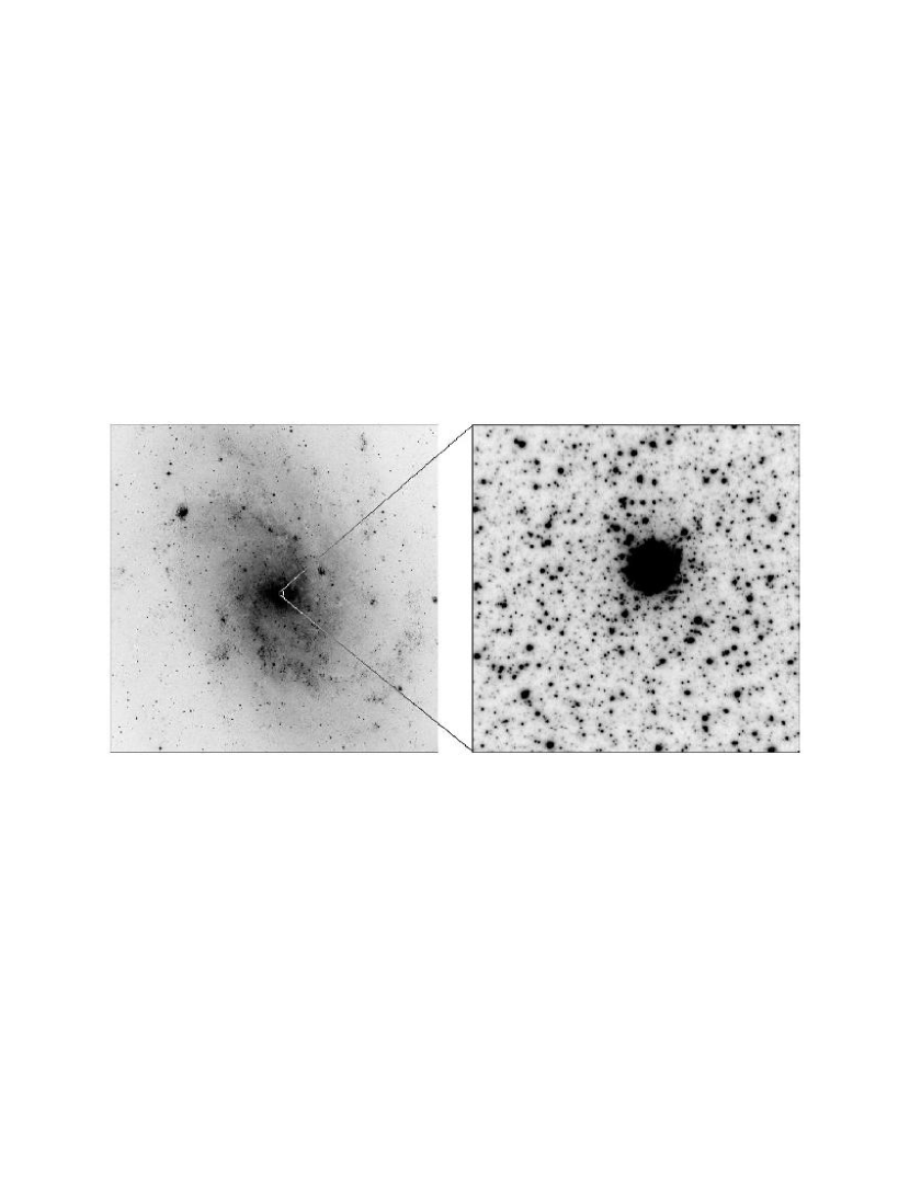
Figure 1: Relative size and location of our infrared image. The left image is a $30^{\prime}$ red Digitized Sky Survey image centered on M33, and on the right is our $\sim 22^{\prime\prime}$ $H$-band Gemini-North image. North is up and east is to the left. The faintest stars visible in the infrared image have $H\sim 20.5$.

We obtained sky observations for background subtraction in a blank field $\sim 45^{\prime}$ SE of the nucleus ($\alpha=$01:34:57, $\delta=+$29:57:20, J2000). The typical observing pattern was to take two sky dithers, four dithers on the nucleus, two skys, etc. With this technique the sky frame is constructed from the combination of the pairs of sky frames before and after each observation, and hence each two-dither sky set is used for both the preceding and following galaxy observations. The sky sets used $3.2^{\prime\prime}$ dithers, while the galaxy sets used $1.3^{\prime\prime}$ dithers.

UKIRT photometric standard stars were observed each night, although possibly not quite as frequently as the authors would have liked. The September night had one standard before and one after our observations; the October night had two before; and the December night had two before and one after. These standards were typically observed with 5 second exposure times, implementing a five position dither pattern moving the star in $10^{\prime\prime}$ steps.

Table 1: Dates & Number of Observations

Date	N($J$)	N($H$)	N($K^{\prime}$)
2000-09-27	8	0	12
2000-10-25	8	0	8
2000-12-22	0	19	0

Image quality was extremely good. We used the IRAF gemseeing procedure to estimate the full-width at half-maximum (FWHM) on all 55 images. The results shown in Figure 2 are the average FWHMs measured on the same $\sim 50$ hand-selected stars on all frames. The $K^{\prime}$-band images have a mean seeing of $0.13^{\prime\prime}\pm 0.02^{\prime\prime}$, $H$-band obtained $0.12^{\prime\prime}\pm 0.02^{\prime\prime}$, while the $J$-band images are slightly worse and more variable with a mean seeing of $0.19^{\prime\prime}\pm 0.03^{\prime\prime}$. The superior image quality at longer wavelengths is a consequence of the increased coherence length of the atmosphere ($\propto\lambda^{6/5}$). The image size does not vary significantly across the field, although the PSF morphology has a systematic dependence on the azimuthal angle around the nucleus of M33, which was used as the AO reference. For comparison, the diffraction limits of an 8m telescope are $0.04^{\prime\prime}$, $0.05^{\prime\prime}$, and $0.07^{\prime\prime}$ at $J$,$H$, and $K^{\prime}$ respectively.

The FWHM, however, is not the best measurement of image quality since most AO images consist of a tight core superimposed on much broader emission. We therefore also recorded the gemseeing task’s estimates of various encircled energy diameters (EED). We found that the 50% EED is approximately twice the FWHM, while the average 95% EEDs are $0.82^{\prime\prime}$, $0.60^{\prime\prime}$, and $0.65^{\prime\prime}$ at $J$, $H$, and $K^{\prime}$ respectively.

Figure 2: The observed distribution of image quality for all observations. The upper panel shows the measured FWHM in arcseconds for the $J$-band frames. Similar histograms for the $H$ and $K^{\prime}$ bands are displayed in in the middle and lower panels respectively. The average FWHM and the total number of frames measured in each band is given in the upper right corner of each panel.

3 Data Reduction & Photometry

We reduced our data using the Gemini package of tools in IRAF. The procedure involves division by a normalized lamps on – lamps off dome flat field, and subtraction of a sky frame constructed from sky observations before and after each galaxy observation. A constant equal to the median of the sky frame was then added back to the image to restore the original sky level and maintain the noise characteristics of the frame.

Photometry was performed with Peter Stetson’s suite of software. Object detection was done on a combined image made up of all the dithers of all the bands. We then used daophot (Stetson, 1987) to determine point spread functions (PSFs) for each dither of each band using isolated stars. We used a quadratically variable model PSF with a 25 pixel ($0.5^{\prime\prime}$) radius; an alternate run using a larger 50 pixel ($1^{\prime\prime}$) radius PSF, yielded little difference in the photometry, while taking a significantly larger amount of processing time. Instrumental magnitudes were measured using the allframe PSF fitting routine (Stetson, 1994) which simultaneously fits PSFs to all stars on all dithers. daogrow (Stetson, 1990) was then used to determine the best magnitude in a $0.5^{\prime\prime}$ radius aperture.

Our first attempt at calibrating the data used the photometric standards which were observed for us. We measured each standard using simple aperture photometry with a $0.5^{\prime\prime}$ radius aperture, and a sky annulus from $2^{\prime\prime}$ to $3^{\prime\prime}$. Due to the small number of observed standards, we combined the measurements from all three nights. This gave us three $J$ standards and four $K^{\prime}$ standards for the September and October nights, and three $H$ standards for the December night. Unfortunately, there are no published $K^{\prime}$ measurements for UKIRT standards. We therefore estimated $K^{\prime}$ for each of the observed standards using the ($H-K$) color and the transformation of Wainscoat & Cowie (1992). Using the median combination of these measurements, we estimated our photometric zero point with uncertainties of 0.02 magnitudes in $H$ and $K^{\prime}$, and 0.04 magnitudes in $J$. We then converted our science $K^{\prime}$ measurements to $K$ based on each star’s $(H-K^{\prime})$ color using a transformation derived from the data published by Wainscoat & Cowie (1992). The last step was to convert our measurements to the CIT/CTIO photometric system using the transformation equations of Hawarden et al. (2001).

This initial calibration seemed to work acceptably for the $J$ and $H$ bands, but not for $K$. Evidence of the failure was in the disagreement ($\sim 0.3$ magnitudes) with previously published data for the stars in the inner region of M33. Specifically, with the $K$-band measurements of bright stars measured by Davidge (2000a), and an equal offset in the $K$-band surface brightness measurements published by Regan & Vogel (1994). One possible cause of the problem is an inadequate transformation between $K$ and $K^{\prime}$. The Wainscoat & Cowie (1992) transformation was published in a paper describing the original $K^{\prime}$ filter. Yet even a cursory comparison of the $K^{\prime}$ filter transmission curve published for QUIRC and that in the Wainscoat & Cowie (1992) article reveals that they are very different. As an example, the original filter had a peak transmission of $\sim 80$%, while the QUIRC $K^{\prime}$ filter peaks over 95%.

To overcome this problem we had to find alternate “standards”, preferably ones which had been observed before. For this purpose, we matched observations of 31 stars in common with the photometry published by Davidge (2000a). We examined the difference between his $K$ band observations (UKIRT photometric system) and our instrumental $K^{\prime}$ for any dependence on $(J-K)$ or $(H-K)$ color, but found no significant trend. We therefore adopted the mean difference as our photometric zero point and conversion to the $K$-band. The uncertainty in this zero point is 0.02 magnitudes. A more detailed discussion of the comparison between these two datasets can be found in Section 8.1.

With the measurements finally calibrated we could construct our final photometry list. Since our transformation to the CIT/CTIO system requires both $(J-K)$ and $(H-K)$ color information, we had already selected out only stars which have measurements in all three bands. In addition, each star had to have been detected on at least five dithers in each band, and the final error had to be less than 0.25 magnitudes. This gave us a list of 3716 objects over the entire frame. After ignoring objects detected within $3^{\prime\prime}$ of the center of M33 because of severe crowding and incompleteness (see Section 5.1), we were left with a final photometry list of 3308 measurements, covering an area of 416 square arcseconds.

When converting to absolute or bolometric magnitudes, we will use the distance and reddening to M33 as determined by Freedman, Wilson & Madore (1991) from observations of Cepheid variables. They find a true distance modulus of $(m-M)_{0}=24.64$ (850 kpc, $1^{\prime\prime}=4.1$ pc), assuming 18.5 for the LMC. They also measure the M33 reddening to be $E(B-V)=0.1$, assuming 0.1 for the LMC, and a ratio of total-to-selective extinction of $R_{V}=3.1$. These values translate to an infrared extinction and reddening of $A_{K}=0.03$ and $E(J-K)=0.05$. We note, however, that Sarajedini et al. (2000) have recently calculated a slightly farther distance of 930 kpc, $(m-M)_{0}=24.84\pm 0.16$, using RR Lyrae’s in two halo clusters.

4 Surface Brightness Decomposition

In order to obtain accurate surface brightness measurements, we started with our reduced frames, and subtracted off the constant sky value which had been added previously to maintain each frame’s noise characteristics. We then converted each frame to count rates, since some of the frames had slightly different exposure times. The resulting set of images in each band were averaged together to create the final images.

We used the xvista annulus routine to compute azimuthally averaged radial surface brightness profiles. Assuming an inclination of 56°(Zaritsky, Elston & Hill, 1989) and a position angle of 23° for M33, the routine defines elliptical annuli to be used as the averaging paths, in effect calculating the deprojected surface brightness profile assuming a circular disk. With 2 pixel wide annuli ($0.04^{\prime\prime}$), we were able to calculate the surface brightness profile out to $15^{\prime\prime}$. We then combined our surface brightness measurements with those of Regan & Vogel (1994) which span from $7^{\prime\prime}$ to $18^{\prime}$. The resulting $K$-band profile is shown in Figure 3. There are three Regan & Vogel (1994) points in the region of overlap ($7^{\prime\prime}-15^{\prime\prime}$), and in this region the average difference between the two datasets is less than 0.01 magnitudes arcsecond^-2. Note that since the surface brightness information is extracted directly from pixel values, the profile is unaffected by image blending, even in the most crowded regions.

Using this combined surface brightness profile ($0.12^{\prime\prime}<r<18^{\prime}$), we have performed a simple bulge/disk decomposition. We assume an exponential disk (eqn. 1) with a central intensity $I_{0}$ and a disk scale length $R_{d}$, and a de Vaucouleurs $r^{1/4}$ bulge (eqn. 2) with an effective radius $R_{e}$ and an intensity $I_{e}$ at $R_{e}$. The factor $a=\sqrt{(1+\cos^{2}i)/2}$ is a correction factor for deprojecting a spherical bulge.

The best fitting 2-component model is illustrated in the left panel of Figure 3 with a solid line. The disk has a central surface brightness of 17.16 magnitudes arcsec^-2, and a scale length $R_{d}=4.87^{\prime}$. The bulge is very compact, with an effective radius $R_{e}=1.1^{\prime\prime}$, where the surface brightness is 13.87 mag arcsec^-2.

The results of the fit are not very encouraging for this oversimplistic disk + bulge model. It is very clear that M33 has a strong compact spheroid component which becomes dominant over the disk at $r\lesssim 5^{\prime\prime}$. However, the best fit parameters are neither a good fit to the inner bulge, nor to the disk between $1^{\prime}-7^{\prime}$.

$$I_{disk}(r)=I_{0}\exp(-r/R_{d})$$ (1)

$$I_{bulge}(r)=I_{e}\exp\{-7.67[(ar/R_{e})^{1/4}-1]\}$$ (2)

$$I_{core}(r)=I_{s}\exp\{-b_{n}[(ar/R_{s})^{1/n}-1]\}$$ (3)

A simple alternative is to add a third component to our model. We thus try an exponential disk + $r^{1/4}$ spheroid + Sersic core (Sersic, 1968). The Sersic function (eqn. 3) is parameterized with an effective radius $R_{s}$, an intensity $I_{s}$ at $R_{s}$, and the shape index $n$ ($b_{n}\approx 1.9992n-0.3271$). The variable power-law index $n$ gives the Sersic function an extra degree of freedom over the more constrained exponential or $r^{1/4}$ profiles.

The results of this three component model are shown on the right side of Figure 3 and the parameter values are listed in Table 2. Not surprisingly, this yields a significantly better fit than for the two component model. The central peak in surface brightness is well described by the Sersic function, the disk is $\sim 0.5$ magnitude fainter, and the spheroid explains the excess luminosity seen inside $1^{\prime}$. Note that we list only the parameters derived from the $H$- and $K$-band images. The $J$-band image quality was inadequate to accurately model the very narrow core component.

Figure 3: The azimuthally averaged $K$-band surface brightness profile ($0.12^{\prime\prime}<r<15^{\prime\prime}$) combined with measurements from Regan & Vogel (1994) ($7^{\prime\prime}<r<18^{\prime}$). The left panel shows the results of a simple 2-component exponential disk (long dashed line) + $r^{1/4}$ bulge (short dashed line) decomposition. The right panel adds a Sersic core (dotted line) as a 3rd component to the decomposition.

Table 2: Three Component Model Parameters

Parameter	$H$-band	$K$-band
Disk scale length, $R_{d}$	$5.58^{\prime}$	$5.67^{\prime}$
Disk central SB, $I_{0}$	18.13	17.75
Spheroid effective radius, $R_{e}$	$39.99^{\prime}$	$22.36^{\prime}$
Spheroid SB @ $R_{e}$, $I_{e}$	24.08	23.40
Core effective radius, $R_{s}$	$0.61^{\prime\prime}$	$0.68^{\prime\prime}$
Core SB @ $R_{s}$, $I_{s}$	13.03	12.73
Core shape index, $n$	2.21	2.07

Note. — Surface brightnesses are in mag/arcsec².

These disk and spheroid parameters are similar to those derived by Regan & Vogel (1994) based on their $r>7^{\prime\prime}$ data alone. They found a disk scale length of $6.1^{\prime}\pm 0.3^{\prime}$ at $H$ and $5.8^{\prime}\pm 0.4^{\prime}$ at $K$, with a central surface brightnesses of $H=18.21$ and $K=17.80$ mag/arcsec². However, since they were only using a two-component model (and excluding the inner $6^{\prime\prime}$), they derived a brighter, more compact spheroid with $R_{e}=8^{\prime}$, $I_{e}(H)=22.84$, and $I_{e}(K)=22.63$ magnitudes arcsecond^-2. Their more compact spheroid is also in agreement with the $8.5^{\prime}$ spheroid effective radius found by Minniti, Olszewski & Rieke (1993).

Kent (1987) studied the surface brightness profile of M33 in the visible, and found a larger exponential disk scale length of $9.6^{\prime}$. He also realized that the profile was too high for just an exponential disk inside $3^{\prime}$, but he dismissed it due to the presence of visible spiral structure, concluding that the disk is non-exponential in the center.

If our three component model is taken literally, it implies that virtually our entire field is spheroid dominated. At $3.6^{\prime\prime}$ the spheroid and central core have equal surface brightness, which is 0.7 magnitudes brighter than that of the disk. At the edges of our field, $r\sim 15^{\prime\prime}$, the disk and spheroid surface brightness become nearly equal. If this is correct, and the spheroid and disk are composed of different stellar populations, we may be able to detect a very small change in the composite population as a function of radius (see Section 9).

We have also estimated the size of the core from our combined $K^{\prime}$ image. This image has better image quality than the $J$ band, and is not saturated like the $H$ images. On this image the nucleus has a FWHM of $0.30^{\prime\prime}$, compared to the stars which have a width of $0.13^{\prime\prime}$. Thus we estimate that the nucleus has a width in $K^{\prime}$ of less than $0.27^{\prime\prime}$. We give this value as an upper limit since we do not attempt to correct for the nonlinearity of the array in the very core ($r<0.1^{\prime\prime}$) where the count rate is too high for the exposure time. This value seems in line with the increasing core size with wavelength measured by Gordon et al. (1999) using HST. They find a core FWHM of $0.12^{\prime\prime}$ with the F300W filter, $0.20^{\prime\prime}$ with the F555W filter, and $0.25^{\prime\prime}$ with the F1042 filter.

Although we could not measure the nuclear luminosity because the central pixels of our images were saturated, we can make an estimate based on our surface brightness fits. Integrating the “core” component from the best-fitting three component model, we find a total luminosity of $M_{H}=-14.03$ and $M_{K}=-14.54$. Assuming $M_{K\odot}=+3.33$, this corresponds to $L_{K}=1.4\times 10^{7}L_{\odot}$.

5 Artificial Star Tests

In order to understand the completeness of our observations and estimate the importance of blending, we have performed a series of tests using artificial data. The traditional completeness tests inject artificial stars into the observed frames; the efficiency and accuracy of their recovery give information about the completeness of the observations (Stetson & Harris, 1988). This method is straightforward and easy to use, but is limited to primarily uncrowded fields. The more complex artificial field technique creates an entire frame containing millions of artificial stars to match the observations (Stephens et al., 2001). This method is especially useful in very crowded fields, providing important constraints on the underlying stellar population.

However, since photometry of the entire set of 55 $1024\times 1024$ pixel frames can be quite time consuming, taking many days to complete, our artificial star tests were instead run on the final combined $JHK$ images. To validate this shortcut, we have compared photometry obtained from the combined images with that from the simultaneous measurements of the 55 individual dithers. Tests show that these two techniques are nearly identical, except for the faintest stars, where the photometry performed on the individual frames tends to be more complete. This can be seen in Figure 4, which shows luminosity functions derived from each of the two methods. The LF obtained from the individual frame photometry (solid line) rolls over approximately one magnitude fainter than the LF from the combined frames (beaded line), even though they both go to about the same depth.

Figure 4: Comparison of luminosity functions obtained from photometry of all 55 individual, uncombined dithers (solid), and photometry from the final combined images (beaded). Both LFs only include stars measured farther than $3^{\prime\prime}$ from the center of M33. The LFs are virtually identical except at the faint end, where the combined frame photometry turns over at $K\sim 20.5$, while the photometry performed on individual dithers does not turn over until $K\sim 21.5$.

5.1 Traditional Completeness Tests

Starting with the three ($JHK^{\prime}$) final combined images, we used the daophot addstar routine (Stetson, 1987) to insert 361 artificial stars into each image. These stars were arranged in a grid of $19\times 19$, with a spacing of $2\times R_{PSF}+2=52$ pixels ($\sim 1^{\prime\prime}$), to avoid self-crowding. Each star included random Poisson noise, and random sub-pixel coordinate offsets from the aforementioned grid. All stars were input with the same magnitude starting with $K_{i}=17$, and a color based on the mean colors observed in the real frame. We then repeated this process, with the grid of input stars shifted by 26 pixels ($\sim 0.5^{\prime\prime}$). After four trials we had added a total of 1444 artificial stars, each sampling different positions in our frame.

After the addition of the artificial stars, we analyzed these frames in the same manner as our original frames. Stars were detected with daofind and measured on each of the four sets of $JHK^{\prime}$ images simultaneously with allframe. Once the final photometry list was completed, we extracted the colors and magnitudes recovered for the input artificial stars using daomaster to match recovered coordinates with input coordinates, requiring less than a 2 pixel ($0.04^{\prime\prime}$) difference in position.

We repeated this 4-trial procedure for six different integer input magnitudes ($K_{i}=17-22$). We have thus accumulated statistics on a total of 8664 artificial stars. Figure 5 shows the difference between the recovered and input magnitudes as a function of distance from the center of M33 for three of the six input magnitudes ($K_{i}=\{17,19,21\}$). As expected the brightest stars are recovered very accurately, with only a few outliers caused by blends with other bright stars on the frame. Note that an artificial star has to fall almost exactly on top of another star to be brightened but not lost since its position cannot be perturbed by more than $0.04^{\prime\prime}$ to be considered the same input star. Near the center of M33 ($r\lesssim 3^{\prime\prime}$), where the density of stars is very high, Figure 5 shows that almost all of the artificial stars are measured significantly brighter than their input magnitude.

Figure 5: Difference between recovered and input artificial star magnitudes as a function of distance from the center of M33. The upper panel shows stars with an input $K$-band magnitude of 17, the middle shows stars input at $K_{i}=19$, and the lower panel is for $K_{i}=21$.

Since the surface brightness varies across the field, our photometric completeness will also be a function of position on the frame. In Figure 6 we plot the completeness as a function of radius for three of the six input magnitudes. To estimate the completeness, we have counted up the number of recovered stars in radial bins around the center of M33, requiring that the difference between input and recovered magnitudes be less than 0.25. We then divide by the number of artificial stars input into these same bins. The results are averaged over the four trials, and the errorbars show the one sigma dispersion in the range of values obtained over the four trials.

This plot shows several important things about the completeness across our frame. First, the completeness drops off very quickly near the center of M33. The completeness of the brighter stars drops from almost 100% to near zero across a range of only $1^{\prime\prime}$. The fainter stars do not exhibit quite as precipitous a drop, but still make the transition from maximum to minimum values quite quickly; albeit at a larger central distance. Second, the completeness away from the nucleus is relatively constant. Thus it is safe to simply throw away measurements inside some critical radius, where the completeness is low (and the effects of blending are high), and afterwards not worry about spatially varying completeness. Finally, we can measure no stars accurately inside $1^{\prime\prime}$. While some stars are recovered in this region (see Figure 5) their measured brightnesses are all discrepant by more than 0.25 magnitudes.

Figure 6: Completeness as a function of distance from the center of M33 for three different input magnitudes: $K_{i}=17$ (solid), $K_{i}=19$ (short dashed), and $K_{i}=21$ (long dashed). We have required that the absolute difference between the recovered and input magnitudes be no greater than 0.25 magnitudes.

Figure 7 shows the photometric completeness as a function of the brightness of the input artificial stars. Here again we require that the recovered magnitude be no more than 0.25 magnitudes different than the input magnitude. Since Figure 6 shows that the negative effects of the core of M33 are constrained to the inner $\sim 3^{\prime\prime}$, we split this figure into two components. The solid line shows the completeness measured for all stars outside $3^{\prime\prime}$, which are again lower limits on the completeness since measured on the combined frames, while the science photometry was performed on all 55 individual frames simultaneously. The dashed line is for all objects measured closer than $3^{\prime\prime}$ to the center of M33, and shows that the photometry inside $3^{\prime\prime}$ is severely degraded at all magnitudes.

Figure 7: Completeness as a function of the input $K$-band magnitude plotted for regions farther than $3^{\prime\prime}$ (solid) and closer than $3^{\prime\prime}$ (dashed) from the center of M33. To be counted as recovered, a star had to be measured to within $0.04^{\prime\prime}$ and 0.25 magnitudes of its input position and magnitude.

5.2 Artificial Fields

We have created a completely artificial field to match our M33 observations. We processed and measured this field in exactly the same manner as the real observations. Since we know both the measured and true magnitude and color of every star in the artificial field, we can quantify our errors and try to estimate the true properties of the observed stellar population being modeled, free from observational effects.

Starting with blank frames with the appropriate amount of Poisson noise, we add 8 million stars using spatially variable PSFs modeled from the real data. The stars follow the observed M33 radial distribution, specifically the sum of the three component $K$-band decomposition of §4.

The input stellar population is chosen to match the colors and luminosity function observed in our M33 field. The input colors are the mean colors observed for stars with $r>3^{\prime\prime}$, and calculated at 0.5 magnitude intervals. The input luminosity function follows a power law distribution with a slope $d(logN)/dM_{K}=0.37$ (as is measured in §7), extending from $-8.8<M_{K}<5$. We add stars until the recovered LF of the simulation approximately matches the recovered LF of the real observations. In this case we added 8 million stars, which gives us slightly fewer recovered stars than in the real frame, 2677 artificial vs 2802 real, however as Figure 8 shows, we get a very good match over most of the range of luminosities.

The artificial frames were then processed and measured in the same manner as the real data, namely finding stars on a combined image with daofind, modeling the PSF from isolated stars, and simultaneous PSF-fitting photometry with allframe.

The resulting $M_{K}$,$(J-K)$ and $M_{K}$,$(J-H)$ CMDs are shown in Figure 9. Here we have included all objects measured on the frame to show how well the simulation reproduces the observations, including blended objects located within $r=3^{\prime\prime}$ (half-size points). We will discuss the implications of these simulations when we attempt to quantify the effects of crowding on our photometry.

Figure 8: Luminosity functions recovered from the simulated M33 frame (solid line) and the real combined frames (beaded line). In total, we measured 2802 objects in the real (combined) frame and 2677 in the simulation ($r>3^{\prime\prime}$).

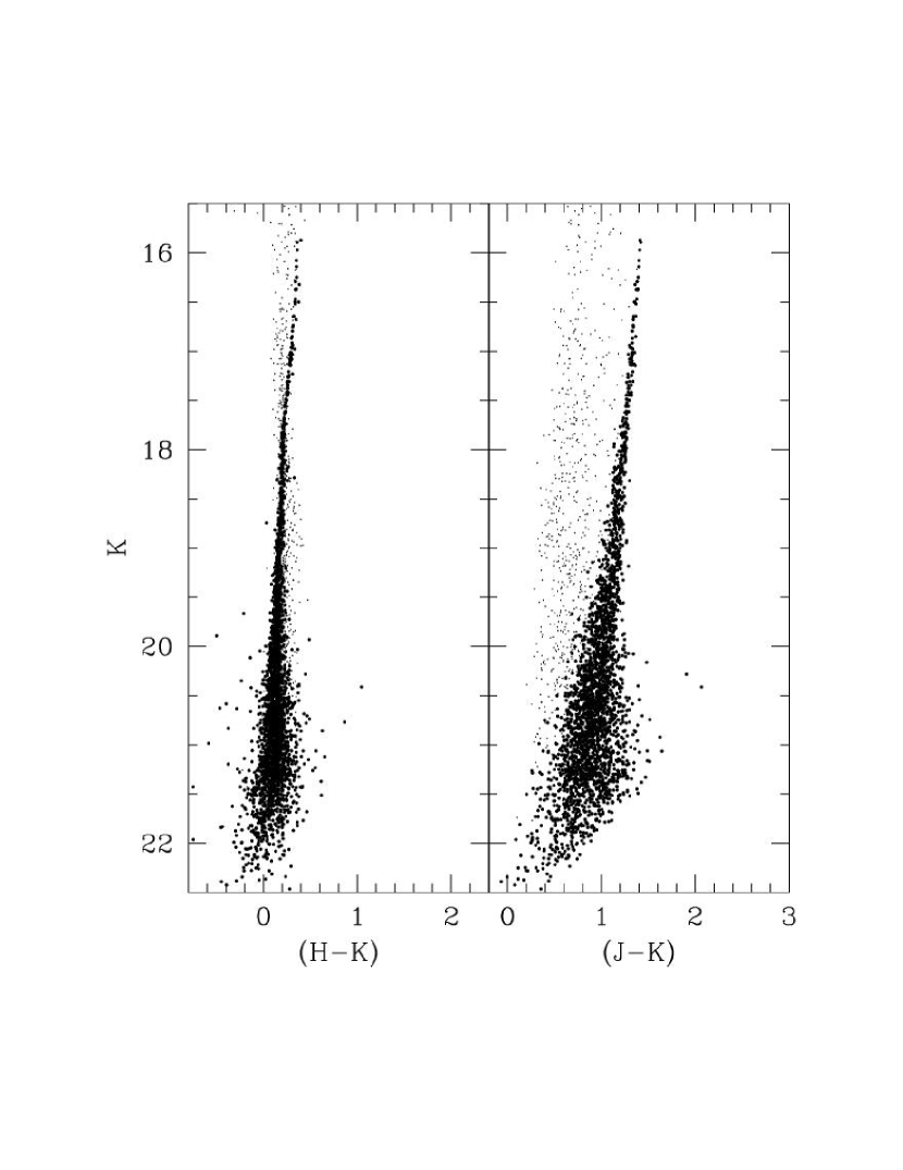
Figure 9: The CMDs measured from the simulated field. Half size points indicated objects measured with $r<3^{\prime\prime}$.

6 Color – Magnitude Diagram

The CMD of our M33 field is shown in Figure 10. Here we have omitted objects measured within $3^{\prime\prime}$ of the nucleus which are mostly blends of fainter, bluer stars as indicated by their characteristic blueward and upward shift from the main giant branch locus (see Figure 9). We have shown in Section 5.1 that nearly all objects detected close to the nucleus are blended, and that $3^{\prime\prime}$ is approximately the boundary outside of which accurate photometry can be achieved. We thus take $3^{\prime\prime}$ as the dividing radius between “good” and “bad” photometry. The resulting CMD for $r>3^{\prime\prime}$ is relatively clean; we interpret the gap at $K\sim 18.2$ as the tip of the red giant branch (RGB), and stars extending to $K\sim 16$ as the asymptotic giant branch (AGB). We compare our CMD with measurements by others in Section 8.

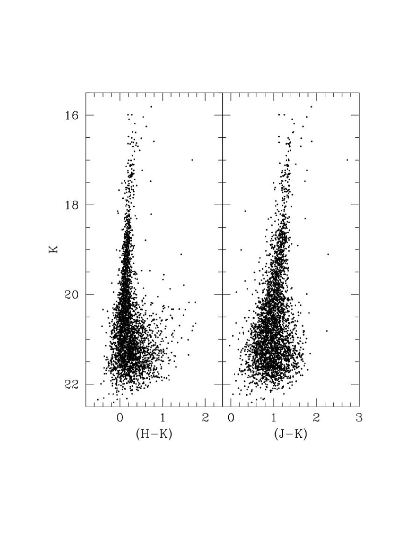
Figure 10: Color magnitude diagrams for our M33 field ($r>3^{\prime\prime}$) obtained from simultaneous photometry on the individual dithers.

6.1 Metallicity

The slope of the RGB is very sensitive to the metallicity of the population. Kuchinski et al. (1995) and Kuchinski & Frogel (1995) have used this fact to develop a metallicity indicator using the slope $(\Delta(J-K)/\Delta M_{K})$ of the infrared RGBs of the upper five magnitudes ($-1>M_{K}>-6$) of Galactic globular clusters . Their relation is given in Equation 4.

$${\rm[Fe/H]}=-2.98-23.84\times slope_{GB}$$ (4)

To apply this relation, we measure the RGB slope in the range $-3.25>M_{K}>-6$, iteratively throwing away $3\sigma$ outliers; the faint limit of $M_{K}=-3.25$ is where the measured LF begins to turn over due to incompleteness (see §7). We find a slope of $-0.114\pm 0.005$, which implies a mean metallicity of [Fe/H]$=-0.26\pm 0.27$. This is our estimate for the average stellar population in the central regions of M33 ($3^{\prime\prime}<r\lesssim 12^{\prime\prime}$). This determination is in agreement with the estimate of [Fe/H]$\sim-0.5$ by O’Connell (1983) using population spectral synthesis of the central $\sim 5^{\prime\prime}$ of M33.

However, as we will show in the next section, there is clearly a young stellar component present in the region imaged. Since the GB slope is also sensitive to age (Tiede, Martini & Frogel, 1997), in the sense that at a constant metallicity the slope increases (gets less negative) with decreasing age. Thus if all the stars (old and young) have the same metallicity, the GB slope will be slightly more positive than for a purely old population, and the Kuchinski relation will give a metallicity which is too low. However, the younger stars are probably more metal rich than the mean of the old population, and hence their GB slope will be closer to that of the older, metal-poor population than if they were of the same metallicity. In short, our metallicity estimate is dependent on both the metallicities and ages of all the stars in the population.

6.2 Population Age

To estimate the age of the youngest stars in our field, we convert our (CIT/CTIO) $K$-band measurements to bolometric luminosities using the corrections of Frogel & Whitford (1987). These corrections were derived for M-giants in Baade’s Window and depend on the dereddened $(J-K)_{0}$ color. The resulting bolometric CMD is shown in Figure 11.

Figure 11: Bolometric color magnitude diagram of the central regions of M33 ($r>3^{\prime\prime}$). Bolometric corrections are from Frogel & Whitford (1987). We assume $(m-M)_{0}=24.64$, $A_{K}=0.03$, and $E(J-K)=0.05$.

Assuming that the few bright stars at the tip of the AGB are members of a young population, we can estimate the age of this population using the relationship between AGB tip luminosity and age. First used by Mould & Aaronson (1979, 1980), this relation makes use of the monotonically decreasing maximum luminosity of the AGB tip with increasing age. Due to the limited number of stars in our field, and the short lifetime of stars on the AGB, this estimate is only an upper limit to the age of the youngest stars.

Stephens et al. (2002) have recalculated the relation between the AGB tip luminosity and age using the ZVAR synthetic CMD code of Bertelli et al. (1992). This program makes use of the stellar evolution models of Bertelli et al. (1994), and the mass-loss prescription of Vassiliadis & Wood (1993). Averaging three different models with different metallicities and binary fractions, they derived Equation 5 for the ages of stars on the AGB tip at different luminosities. Thus by measuring the bolometric luminosity of the AGB tip, one can estimate the age of the youngest stars in the field.

$$\log(Age)= -0.91-7.962M_{bol}-$$ (5)

$$1.7876M_{bol}^{2}-0.12033M_{bol}^{3}$$

The simplest estimate of the age comes from the luminosity of the brightest star in the field. This star has $M_{bol}=-5.658$, which, with equation 5, gives an age of 0.51 Gyr.

If we assume that the intermediate age stars on the AGB can be explained by a single burst of star formation, we can apply the averaging technique of Mould & Aaronson (1982) to overcome small number statistics when estimating the tip of the AGB. Their method is to find the average luminosity of stars on the AGB over the AGB tip of an old population ($M_{bol}\sim-4.5$). By assuming that the distribution of stars along the AGB is uniform, the peak bolometric luminosity for a fully populated AGB should be twice the mean (plus $-4.5$). Using this procedure on the 28 stars brighter than $M_{bol}=-4.5$ we estimate the AGB tip luminosity to be $M_{bol}=-5.41\pm 0.11$ for a fully populated AGB. This luminosity implies an age of $0.79^{+0.18}_{-0.15}$ Gyr for this intermediate age population.

However, looking at the bolometric CMD in Figure 11, it is fairly clear that the stars above $M_{bol}\sim-3.3$ are not uniformly populated along its entire extent. This is probably due to multiple bursts of star formation contributing to the AGB. A careful inspection shows that the AGB is well represented from $-3.4\gtrsim M_{bol}\gtrsim-5$, with a bright tail of stars up to $M_{bol}\sim-5.6$ (see also the luminosity function in Figure 14). The predominant AGB is most likely due to a large burst of star formation around 2 Gyr ago, while the less populated secondary AGB is probably due to an even more recent burst of star formation $\sim 0.5$ Gyr ago.

A similar multi-generation model was proposed for the nucleus of M33 by Gallagher, Goad & Mould (1982) to explain its blue ($U-B$) and red ($B-V$) colors and strong spectral absorption features such as H$\beta$ and H$\gamma$. O’Connell (1983) also argued for multiple epochs of star formation based on the integrated optical spectrum of the inner $10^{\prime\prime}$, and concluded that $\sim 50$% of the $V$-band light originates in stars younger than 1 Gyr, with the youngest generation about $5\times 10^{6}$ years old. Ultraviolet observations agree, Ciani, D’Odorico & Benvenuti (1984) used IUE spectra together with $U,B,V$ photometry of the nucleus to model the stellar population, and found the best-fit model required both a young component with an age of $\sim 10^{7}$ years, and an old component with an age of $\sim 10^{10}$ years. While combining photometric and spectroscopic observations, Gordon et al. (1999) found that the nucleus of M33 is best fit by a $70-75$ Myr old single burst of star formation enshrouded by a significant amount of dust. Most recently, Long, Charles & Dubus (2001) used stellar spectral synthesis to model HST STIS spectroscopy of the nucleus and found that the best fit is with two bursts of star formation 50 Myr and 1 Gyr ago.

We can reject the possibility of field star contamination as an explanation of the bright stars observed in our field using the field star density tabulated by Ratnatunga & Bahcall (1985) which was calculated from the Bahcall and Soneira Galaxy model. To estimate the number of field stars brighter than $K=17$ ($M_{K}=-7.5$), we assume that potential contaminants are field M-dwarfs, they could be as red as $(V-K)\sim 7$. Thus they could be as faint as $V\sim 24$. Ratnatunga & Bahcall (1985) predicts that the number of field stars with $V$ brighter than 25 is $N(V<25)=3.124$ arcmin^-2. Multiplying by the area of our field 0.116 arcmin² gives an upper limit of 0.36 stars brighter than $K=17$ in our field. This means that there is a $<36\%$ chance of finding one star in our field as bright as $K=17$, while we see 27.

7 Luminosity Functions

The luminosity functions (LFs) derived for our field are shown in Figure 12 and listed in Table 3. These include only objects measured farther than $3^{\prime\prime}$ from the center of M33. This region has an area of 416 arcsec². The data have been binned into 0.25 magnitude bins, and the center of each bin is given in column 1. These LFs all show dips at the location of the tip of the RGB ($K\sim 18$).

Figure 12: The luminosity functions measured for $r>3^{\prime\prime}$ binned into 0.25 magnitude bins. The top panel is measured in $J$, the middle in $H$, and the lower in $K$.

Table 3: Luminosity Functions

mag	$N_{J}$	$N_{H}$	$N_{K}$
15.875	0	0	3
16.125	0	1	3
16.375	0	2	4
16.625	0	5	13
16.875	0	9	5
17.125	2	9	16
17.375	0	15	21
17.625	5	23	27
17.875	11	26	14
18.125	7	19	22
18.375	16	25	38
18.625	25	43	68
18.875	19	80	85
19.125	29	92	95
19.375	22	106	105
19.625	49	105	118
19.875	78	142	162
20.125	110	198	208
20.375	116	213	249
20.625	139	256	310
20.875	190	258	359
21.125	226	310	388
21.375	310	357	427
21.625	350	364	349
21.875	385	293	176
22.125	318	207	38
22.375	330	94	5
22.625	286	45	0
22.875	175	10	0
23.125	83	1	0
23.375	27	0	0

We show the absolute $K$-band luminosity function in Figure 13, assuming a distance modulus to M33 of 24.64. For comparison we have also plotted a composite Galactic Bulge luminosity function constructed from Frogel & Whitford (1987) and DePoy et al. (1993) measured in Baade’s Window (BW).

There are two very obvious differences between these two LFs: their bright end extents and their slopes. The M33 LF extends over a magnitude brighter than what is observed in BW. These bright stars, as discussed in Section 6.2, are a result of a young population of stars in the central regions of M33.

The slopes of the M33 and Baade’s Window RGB LFs are also significantly different. We fit each with a single power law, M33 over $-6<M_{K}<-3.25$, and BW over $-6<M_{K}<-1.1$. In M33 we measure a LF slope of $0.312\pm 0.015$, while in BW we find $0.279\pm 0.005$. One possible reason for this difference is the difference in mean ages of the stars in these two regions. M33 contains a mix of young and old stars (e.g. Section 6.2 and the optical-IR CMD in Figure 17), while the Galactic bulge is predominantly an old population. However, Davidge (2000b) has also suggested that the slope of the LF may vary throughout the Galactic bulge. Looking at dereddened LFs of 17 bulge fields, he fits a power law between $M_{K}=-0.5$ and $+1.0$ and finds a range in LF slope of $0.165\pm 0.064<\alpha<0.672\pm 0.225$, with a mean value, obtained by coadding the LFs, of $0.335\pm 0.018$. This mean LF slope obtained by Davidge agrees with what we have measured in the central region of M33, however involves many uncertainties, such as the reddening and the small luminosity range over which the LFs were fit. If indeed galaxy LFs are variable, as Davidge’s data suggests, deeper high-resolution imaging of M33 may prove one of the most robust ways to verify this effect.

Figure 13: Comparison between luminosity functions measured in M33 (solid line), and the bulge of our Galaxy viewed through Baade’s Window (beaded line). The M33 LF is constructed by placing the stars measured outside a $3^{\prime\prime}$ radius into 0.25 magnitude wide bins. The BW LF is the combination of the bright end of Frogel & Whitford (1987), and the faint end of DePoy et al. (1993), and has been scaled to match the number of M33 counts in the magnitude range $-7.5<M_{K}<-6$. This plot assumes that $(m-M)_{M33}=24.64$ and $(m-M)_{BW}=14.5$

Finally we present the bolometric luminosity function derived from our observations in Figure 14. The data cover 416 square arcseconds, avoiding the central $3^{\prime\prime}$. We have used the bolometric corrections from Frogel & Whitford (1987) which are based on each star’s $(J-K)$ color. Here the dip in the LF at the RGB-AGB transition $(M_{bol}\sim-3.5)$ is especially apparent. The termination of the LF at $M_{bol}\sim-5.5$ is in agreement with the youngest stars on the AGB having an age $\sim 0.5$ Gyr (see Section 6.2).

Fitting a power-law to the LF of the RGB ($-3.25<M_{bol}<-1.5$) we find a slope of $\alpha_{RGB}=0.444\pm 0.029$. If instead we fit the entire luminosity function from the bright end dropoff at $M_{bol}=-5$ to the completeness limit at $M_{bol}=-1.5$, we find a slope $\alpha_{All}=0.499\pm 0.027$. Davidge (2000a) measured the slope between $-5<M_{bol}<-3.5$, a much smaller range than ours, and found a slope of $0.528\pm 0.036$, in good agreement with our determination.

Figure 14: Bolometric luminosity function for all objects measured farther than $3^{\prime\prime}$ from the nucleus of M33. Bolometric corrections are from Frogel & Whitford (1987), where we have assumed that $(m-M)_{0}=24.64$, $A_{K}=0.03$, and $E(J-K)=0.05$. A fit to the RGB (dashed line; $-3.25<M_{bol}<-1.5$) gives a slope of $0.444\pm 0.029$, while fitting the entire LF (dotted line; $-5<M_{bol}<-1.5$) yields a slope of $0.499\pm 0.027$.

8 Comparison with Previous Data

8.1 Davidge (2000a)

Recently Davidge (2000a) has made AO observations of the nuclear regions of M33 with the 3.6m Canada-France-Hawaii Telescope (CFHT). His $\sim 35^{\prime\prime}$ field had a total of 20 minutes exposure time per $JHK$ filter, and his images have a FWHM of $0.34^{\prime\prime}$, about twice the size of the Gemini PSF, which ranged from $0.12^{\prime\prime}$ to $0.20^{\prime\prime}$.

Using his published list of photometry of stars with $K\leq 17$, we have matched up observations of 34 stars. The difference between these measurements is illustrated in Figure 15. Several of the fainter stars are obviously blended in Davidge’s images, however the agreement with the bulk of the sample is quite good. Throwing out three sigma outliers, the average difference between the samples (Davidge – Gemini) is $\Delta J=-0.08\pm 0.02$, $\Delta H=0.08\pm 0.01$, and $\Delta K=0.00\pm 0.02$. The perfect agreement in the $K$-band is of course because we used the same sample of good measurements to determine our $K$-band photometric zero point.

Figure 15: Comparison between measurements made by Davidge (2000a) with the 3.6m CFHT, and the present Gemini-North observations. The mean difference, excluding three sigma outliers is $\Delta J=-0.08\pm 0.02$ and $\Delta H=0.08\pm 0.01$. The $K$-band difference is by definition zero ($\pm 0.02$) since it was used for calibration.

The comparison between our $K$-band LFs is shown in Figure 16. The two LFs agree very well, both in slope and normalization. The most obvious difference is that our LF extends to $K\gtrsim 21.5$, while the Davidge LF rolls over at $K\sim 19$ due to incompleteness. The Davidge LF also has one star $\sim 1$ magnitude brighter than any star in our field, however this is most likely a result of our smaller area not completely sampling the brightest star population. Another difference is that while we see a small dip in the LF due to the tip of the RGB at $K\sim 18$, this feature is not visible in the Davidge LF, probably because it is smeared out due to his reduced photometric accuracy at this level.

Figure 16: Comparison between $K$-band luminosity functions measured in the central regions of M33 with Gemini-North (solid line) and by Davidge (2000a) (beaded line). Our Gemini data only includes objects measured farther than $3^{\prime\prime}$ from the nucleus. Both LFs have been normalized to show the number of stars per square arcsecond per magnitude. The brightest bin ($K=15$) of Davidge’s LF contains only one star with $K=15.03$.

8.2 Mighell & Corder (2002)

Mighell & Corder (2002) have observed the nuclear region of M33 using the Wide Field Planetary Camera 2 (WFPC2) on the Hubble Space Telescope (HST). They have obtained images through the F555W ($\sim V$) and F814 ($\sim I$) filters. Their optical CMD reveals a bright blue main sequence, a red supergiant plume, a very red AGB, and a wide RGB. They interpret this complex CMD as indicative of a mix of young ($<100$ Myr), intermediate age ($\sim 1$ Gyr), and old stellar populations ($>10$ Gyr).

We have matched up their optical WFPC2 observations with our infrared Gemini measurements using daomaster (part of the daophot package, Stetson, 1987) and show the resulting $K-(V-K)$ CMD in Figure 17. For comparison we have overplotted the GB of the old Galactic globular cluster 47 Tuc ([Fe/H] $=-0.76$) from Ferraro et al. (2000). This cluster GB exemplifies the region of this CMD which will be occupied by an old intermediate-metallicity stellar population. The color is fairly red, and the GB tip is well below $K=17.5$. We have also overplotted the mean ridge line of 12 intermediate age Magellanic Cloud clusters from Ferraro et al. (1995). The component clusters have an average SWB-type of IV (Searle, Wilkinson & Bagnuolo, 1980), an average $s$ value of 36 (Elson & Fall, 1985), and a mean metallicity of [Fe/H]$=-1.56$ based on the slope and placement of their composite $(V-K)$ GB. This GB exemplifies the location of an intermediate age metal poor stellar population, with the tip of the GB extending over a magnitude brighter than that of 47 Tuc. Lastly, we overplot a 100 Myr, $\sim$ solar metallicity ($Z=0.019$, $Y=0.273$) isochrone from Girardi et al. (2002), which uses a detailed TP-AGB treatment. This isochrone extends even bluer and brighter than the other two RGBs, and can explain the large number of very blue stars with $(V-K)<2$.

Figure 17 makes it clear that, as concluded by Mighell & Corder (2002), there is a lot going on in the central regions of M33. There appear to be young blue main sequence stars and red supergiants, an intermediate age GB similar to the MC clusters, and an evolved GB like that of the Galactic cluster 47 Tuc. For a discussion of previous work on this topic see the end of Section 6.2. Unfortunately, degeneracies between age and metallicity make it very difficult to quantitatively describe the mix of stellar populations based on our photometric dataset alone. (O’Connell, 1982; Worthey, 1994)

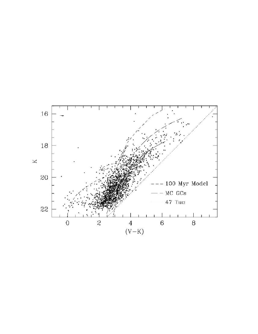
Figure 17: Combined optical (WFPC2, Mighell & Corder, 2002) and infrared (Gemini-North) color-magnitude diagram. For comparison we have overplotted the GB locus of the Galactic globular cluster 47 Tuc ([Fe/H]$=-0.76$) from Ferraro et al. (2000), the mean ridge line of 12 intermediate age Magellanic Cloud clusters from Ferraro et al. (1995), and a 100 Myr solar metallicity isochrone from Girardi et al. (2002). The overplotted lines have been reddened to match the assumed reddening in M33, which is illustrated by the small arrow in the upper left corner. The limiting magnitude of the optical photometry at $V=25$ is marked by the dotted line.

9 Radial Variations in M33 Populations

In Section 4 we showed that the best 3-component fit to the surface brightness profile includes spheroid and disk components whose relative contributions vary significantly across our field. If this model is correct, and these two populations are sufficiently different, we may be able to detect this variation by looking for a radial dependence of the slope and extent of the luminosity function, and in the morphology of the color-magnitude diagram.

To test this hypothesis, we have divided our field into four equal-area rings around the center of M33. The results are summarized in Table 4 which lists the properties measured in each ring as well as in the entire field. The first two columns of Table 4 give the limits of each ring, chosen so that each has an area of 50 arcseconds² (also illustrated in Figure 18). The third column ($N$) lists the number of stars measured in each ring. The fourth and fifth columns give the giant branch slope ($m_{GB}$) and the luminosity function power-law slope ($\alpha_{LF}$), both measured from $-3.25>M_{K_{0}}>-6$. The last column gives the brightest star measured in each annulus as an estimate of the tip of the AGB. The results for the entire frame are listed in the last row of the table, and marked $r>3^{\prime\prime}$.

Figure 18: The radial distribution of stars measured in the central region of M33. The dashed lines at $r=$ 3, 5, 6.4, 7.5, and 8.5 arcseconds indicate the boundaries of the regions used in the analysis of Section 9.

Table 4: Variations with Radius

$R_{1}$	$R_{2}$	$N$	GB slope	$\alpha_{LF}$	$M_{bol}$(AGBT)
3.0	5.0	484	$-0.118\pm 0.012$	$0.260\pm 0.029$	$-5.32$
5.0	6.4	467	$-0.082\pm 0.013$	$0.333\pm 0.036$	$-5.02$
6.4	7.5	444	$-0.115\pm 0.012$	$0.338\pm 0.055$	$-5.17$
7.5	8.5	424	$-0.094\pm 0.012$	$0.316\pm 0.039$	$-5.29$
$r>3^{\prime\prime}$		3308	$-0.114\pm 0.005$	$0.312\pm 0.015$	$-5.66$

9.1 Variations in the Stellar Distribution

In this section we analyze both the radial distribution of stars, as indicated by the Kolmogorov-Smirnov statistic (KS-test), and the distribution of stellar luminosities as measured by fitting power-law luminosity functions as well as the KS-test. The radial distribution of measured $K$-band magnitudes are shown in Figure 18, which illustrates the continuum of stellar luminosities over the field.

First we perform the KS-test on the radial positions of stars plotted in the optical-IR CMD (Figure 17). Here we have divided the stars into two groups: blueward of the intermediate age Magellanic Cloud cluster locus, which we call “young”, and redward of the MC cluster locus, which we call “old”. For both groups we consider stars only brighter than $K=21$ to minimize the effects of incompleteness. When considering all stars from $3^{\prime\prime}$ to $14^{\prime\prime}$, the KS-test shows a marginal difference ($P=0.01$) between the radial distribution of the “young” and “old” stars, however this difference arises in the very central regions, and is most likely due to incompleteness in this more crowded region. When we limit the test to stars outside $4^{\prime\prime}$, the radial distributions of the two groups become nearly indistinguishable ($P=0.08$). Thus based on the stars from $4^{\prime\prime}$ to $14^{\prime\prime}$ in the optical-IR CMD, we would conclude that the radial distributions of “young” and “old” stars are identical.

If instead, we consider our whole sample of infrared measurements, and are more selective in our choice of “young” stars, namely bluer than $(J-K)=0.6$ and brighter than $K=21.5$, these stars appear to lie at larger radii than the remainder of the population. Performing a KS-test on this small subsection of the CMD, from $4^{\prime\prime}$ to $14^{\prime\prime}$, gives a very low probability ($P=2.7E-6$) that these stars have the same radial distribution as the other stars. However the observed difference arises at primarily large radii ($r\gtrsim 9^{\prime\prime}$). If the KS-test is run from $4^{\prime\prime}$ to $10^{\prime\prime}$ the significance completely disappears. We mention this result as an aside because it is only evident in the outermost regions of the field, where the completeness due to dithering is difficult to calculate and the probability for systematic effects caused by the large distance from the wavefront reference source (nucleus) is highest.

Mighell & Rich (1995) did find significantly different radial distributions of young and old stars in the central $\sim 70^{\prime\prime}$ of M33 based on optical HST-PC observations. Specifically they found that the younger Pop I stars preferentially lie farther from the nucleus than the more centrally concentrated older Pop II stars.

Next we look at the luminosity functions measured in each of the four rings defined in Table 4 and illustrated in Figure 18. We fit a power-law to the RGB from $-6<M_{K_{0}}<-3.25$ and find that there is no significant change across the field, and that the slopes determined are all consistent with that measured for the entire field: $\alpha=0.312\pm 0.015$. A more rigorous analysis using the KS-test verifies this general result. These tests show that based on the distribution of stellar luminosities in each of the four annuli, as well as on the radial distribution of stars of different luminosities (binned into 1-magnitude bins), all stars are consistent with being drawn from the same population.

McLean & Liu (1996) obtained similar results for the inner disk of M33. Comparing AGB stars brighter than $K\sim 18$ in two regions, $45^{\prime\prime}<r<1.5^{\prime}$ and $1.5^{\prime}<r\lesssim 4^{\prime}$, they found no significant difference between the luminosity functions except for the presence of luminous supergiants in the outer region.

Figure 19: Luminosity functions for four equal area rings around M33. A power-law has been fitted to each in the range $-6<M_{K0}<-3.25$ and is overplotted with a dotted line. The slopes are given in the upper left corner of each panel.

9.2 Variations in the CMD

The CMDs of each of the four rings are displayed in Figure 20. The radial limits of each are at the top of each CMD, and the number of objects found in each ring is printed in the bottom right corner. Using the same technique which we used to estimate the mean metallicity of the stellar population in Section 6, we now measure the slope of the GB in each ring. As before, the iterative linear fit is only to data with $-3.25>M_{K0}>-6$, and ignores three sigma outliers.

Figure 20: Color-magnitude diagrams for rings of equal area around M33. The number of stars in each ring is given in the lower right corner of each panel.

The results of the GB fitting are listed in column 4 of Table 4. We find that based on the slope of the giant branch, the mean metallicity of each annulus is consistent with that of the entire field. This is similar to what has been observed in the inner Bulge of our Milky Way ($R<560$ pc), which shows no evidence for a gradient along the major or minor axes (Ramírez et al., 2000).

Although we have not detected a gradient in the stellar properties in the inner $\sim 10^{\prime\prime}$, we have nonetheless helped fill in the gap between the metallicity gradient observed in the disk of M33 (Henry & Howard, 1995; Kwitter & Aller, 1981; Searle, 1971), and low abundance measurements for the nuclear region, most recently [Fe/H]$=-1.2\pm 0.5$ ($0.5^{\prime\prime}>r>1^{\prime\prime}$) based on the CO index by Davidge (2000a).

10 Luminous Stars and Blending in M33

As Renzini (1998) has pointed out, meaningful photometry can only be obtained for stars brighter than the luminosity contained in each resolution element. We have calculated the enclosed luminosity in M33 for five different imaging resolutions ($0.13^{\prime\prime}$, $0.34^{\prime\prime}$, $0.75^{\prime\prime}$, $1.5^{\prime\prime}$, and $3^{\prime\prime}$), assuming that the size of the resolution element is defined by the FWHM. Figure 21 shows the corresponding limiting $K$-band magnitude as a function of surface brightness. This plot shows that at $\mu_{K}\sim 16.8$, the surface brightness over most of our field, the faintest stars which we can accurately measure with our $\sim 0.13^{\prime\prime}$ resolution have $K\sim 21.5$. This is in very good agreement with the observed limit of our photometry (e.g. Figure 10).

Even more useful perhaps, is a plot of the limiting magnitude due to blending as a function of spatial position. For symmetric surface brightness distributions, such as exist around M33, the conversion is relatively simple. Using our three component surface brightness model (Section 4), we have transformed from generic surface brightness to the radial distance from the center of M33 measured in arcminutes. The resulting relations for the same five different resolutions are shown on the right side of Figure 21. Thus for our data, with a resolution of $\sim 0.13^{\prime\prime}$, the faintest stars which we can accurately measure (against blending) at $6^{\prime\prime}$ arcseconds from the center of M33 have $K\sim 21.3$. If we try to measure stars at a distance of $3^{\prime\prime}$, blending will limit our measurements to only stars brighter than $K\sim 20.3$, a full magnitude brighter than we could accurately measure at $6^{\prime\prime}$.

Figure 21: Limits blending places on stellar photometry in M33, as determined by the general rule that meaningful photometry can only be obtained for stars brighter than the luminosity sampled by a single resolution element (Renzini, 1998). The left panel gives the $K$-band magnitude ($K_{lim}$) of the faintest stars which can be accurately measured (against blending) as a function of the background surface brightness for five different imaging resolutions. The right panel uses the surface brightness profile of M33 to convert surface brightness to radial distance from the center of M33. Our resolution is $0.13^{\prime\prime}$, and Davidge (2000a) had a resolution of $0.34^{\prime\prime}$.

Another simple calculation advocated by Renzini (1998) is the estimation of the number of stars in each evolutionary stage per resolution element. This allows one to estimate the severity of blending in any observation. This calculation has several parameters which have a weak dependence on the age, metallicity, and IMF of the stellar population. The ratio of total ($L_{T}$) to $K$-band luminosity ($L_{K}$), and the specific evolutionary flux, $B(t)$, are two such parameters. For our calculation we used $L_{T}/L_{K}=0.36$, and $B(t)=2.2\times 10^{-11}$ stars yr^-1 L_⊙^-1, numbers suitable for a 15 Gyr old, solar-metallicity population.

The results of this calculation for stars within one magnitude of the RGB tip (RGBT) are displayed in Figure 22. In the left panel we show the number of RGBT stars per resolution element as a function of surface brightness for five different imaging resolutions.

The number of blends of two RGBT stars on a frame can be estimated as the square of the number per resolution element (for $N<1$) multiplied by the number of resolution elements in the frame (Renzini, 1998). If the number of RGBT stars per resolution element is greater than one, it should be clear that photometry of stars at or below the level of the RGBT is impossible. At this point only stars several magnitudes brighter than the RGBT can be measured with any accuracy, but then one must face the question of whether the objects measured are real or just blends of many stars, each of which can be as bright as the tip of the RGB.

Stephens et al. (2001) have performed simulations of the blending in their NICMOS observations of globular clusters in M31. They show that severe blending can easily create objects which are several magnitudes brighter than any star in the parent population. Thus one must be very careful when interpreting bright objects measured in a very crowded fields, i.e. where N(RGBT) per resolution element is greater than one.

Figure 22: The number of M33 RGB stars within one magnitude of the RGB tip per resolution element, based on the formulae of Renzini (1998). The probability of a blend of two RGBT stars scales as the square of N(RGBT). The left panel shows N(RGBT) as a function of the background surface brightness for five different imaging resolutions. The right panel uses the surface brightness profile of M33 to convert surface brightness to radial distance from the center of M33.

It might be illuminating to examine a few previous studies of the central regions of M33 keeping Figures 21 and 22 in mind. The most critical, at least in terms of our photometric calibration, are the observations of Davidge (2000a) discussed in Section 3. Plotting his $0.34^{\prime\prime}$ resolution on both Figures, we see that his observations are not significantly affected by blending. The right side of Figure 22 shows that Davidge stays below 1 RGBT star per resolution element until only $2^{\prime\prime}$ from the nucleus, which he (for the most part) steers clear of. Assuming the average distance of his field from the nucleus is $\sim 9^{\prime\prime}$, Figure 21 shows that the limit of accurate photometry (against blending) is $K\sim 19.4$. Since his estimated completeness limit is $K=19$, his photometry is therefore limited by photon noise and not blending.

Checking the observations of McLean & Liu (1996), we see that their infrared $JHK$ observations of the central $7.6^{\prime}$ of M33 had $1.5^{\prime\prime}$ seeing. They divided their observations into a “Central Core Region” going from $45^{\prime\prime}$ to $1.5^{\prime}$, and an “Inner Disk” region, spanning from a radius of $1.5^{\prime}$ to $\sim 4^{\prime}$. Looking at the $1.5^{\prime\prime}$ resolution curve on Figure 21, we find that at $1.5^{\prime}$, their photometric limit imposed by blending is $K\sim 17$, and Figure 22 shows that at this distance there is $\sim 1$ RGBT star per resolution element. Since the number of detected stars in their core region abates at $K\sim 17.5$, they are not trying to go much deeper than blending allows. However, the high density of stars as bright as the RGB tip, and the fact that out to $15^{\prime\prime}$ we only find stars as bright as $K\sim 16$, suggests that some of the brighter ($K\sim 14.5$), bluer [$(J-K)<1.5$] objects they detected in the central region may be blends.

The observations of Minniti, Olszewski & Rieke (1993, 1994) are in a similar situation in terms of blending. With $1.5^{\prime\prime}$ resolution they measured stars as bright as $K\sim 14$ in the inner $2^{\prime}$ of M33. However, as Figure 22 shows, at $2^{\prime}$ with $1.5^{\prime\prime}$ resolution, there are $\sim 0.9$ stars within one magnitude of the tip of the RGB per resolution element. This certainly does not guarantee that these bright objects are blends, but merely shows that the potential for blending is high.

11 Conclusions

We have used Gemini-North to study the stellar populations in the central regions of M33. The surface brightness profiles from $0.1^{\prime\prime}$ to $18^{\prime}$, formed from the combination of our data and those of Regan & Vogel (1994), show that the data need to be modeled using a three-component, core + spheroid + disk model. The best-fit parameters are listed in Table 2.

These high-resolution observations allow us to accurately measure individual stars to $K\sim 21$. Artificial star tests (§5) show that our completeness is relatively uniform across the field (50% at $K=21$), although within $3^{\prime\prime}$ from the nucleus the completeness is dramatically lower due to severe crowding. Artificial fields are used to understand the observational effects associated with adaptive optics measurements in crowded fields.

Based on the slope of the giant branch in the infrared color magnitude diagram, we estimate the mean metallicity to be $-0.26\pm 0.27$ (§6.1). Using the bolometric luminosities and density of stars on the AGB, we hypothesize two bursts of star formation; at $\sim 0.5$ and $\sim 2$ Gyr ago (§6.2). We note however, that this component of young stars may have influenced our metallicity estimate due to the sensitivity of the GB slope on age.

The stellar luminosity function in M33 is shown to be significantly different from that measured in the Galactic Bulge as viewed through Baade’s Window (§7). The difference in their maximum luminosities is due to differences in ages of the two regions. We speculate that this is also the origin of their different slopes as well.

In section 8 we compare our data with previous observations. Recent work by Davidge (2000a) is in good agreement with our data, although our observations go $>2$ magnitudes deeper (§8.1). We also combine our data with optical HST-WFPC2 measurements (Mighell & Corder, 2002), and present the optical-IR CMD in §8.2. This CMD clearly shows that the central regions of M33 are composed of young, intermediate, and old aged stellar populations.

Dividing the inner $\sim 8.5^{\prime\prime}$ ($\sim 35$ pc) into equal area rings around the nucleus, we look for radial variations in the stellar properties (§9). However, based on the distribution of stellar luminosities and the morphology of the CMD, we find that all stars are consistent with being drawn from a single population.

In the last section (§10) we perform calculations to estimate the severity of blending at various imaging resolutions and locations in M33. Using the formulations of Renzini (1998) and our composite surface brightness profile, these calculations call into question some previous claims of very luminous stars in the central regions of M33.

References

- Bertelli et al. (1994) Bertelli, G., Bressan, A., Chiosi, C., Fagotto, F., & Nasi, E., 1994 A&A, 106, 275
- Bertelli et al. (1992) Bertelli, G., Mateo, M., Chiosi, C. & Bressan, A., 1992 ApJ, 388, 400
- Bothun (1992) Bothun, G.D., 1992 AJ, 103, 104
- Ciani, D’Odorico & Benvenuti (1984) Ciani, A., D’Odorico, S., & Benvenuti, P., 1984 å, 137, 223
- Davidge (2000a) Davidge, T.J., 2000a AJ, 119, 748
- Davidge (2000b) Davidge, T.J., 2000b AJ, 120, 1853
- DePoy et al. (1993) DePoy, D.L., Terndrup, D.M., Frogel, J.A., Atwood, B., & Blum, R., 1993 AJ, 105, 2121
- Elson & Fall (1985) Elson, R.A.W. & Fall, S.M., 1985 ApJ, 299, 211
- Ferraro et al. (1995) Ferraro, F.R., Fusi Pecci, F., Testa, V., Greggio, L, Corsi, C.E., Buonanno, R., Terndrup, D.M., Zinnecker, H., 1995 MNRAS, 272, 391
- Ferraro et al. (2000) Ferraro, F.R., Montegriffo, P., Origlia, L. & Fusi Pecci, F., 2000 AJ, 119, 1282
- Freedman, Wilson & Madore (1991) Freedman, W.L., Wilson, C.D., & Madore, B.F., 1991 ApJ, 372, 455
- Frogel & Whitford (1987) Frogel, J.A. & Whitford, A.E., 1987 ApJ, 320, 199
- Gallagher, Goad & Mould (1982) Gallagher, J.S., Goad, J.W., & Mould, J., 1982 ApJ, 263, 101
- Girardi et al. (2002) Girardi, L., Bertelli, G., Bressan, A., Chiosi, C., Groenewegen, M.A.T., Marigo, P., Salasnich, B., Weiss, A., 2002 astro-ph0205080
- Gordon et al. (1999) Gordon, K.D., Hanson, M.M., Clayton, G.C., Rieke, G.H., & Misselt, K.A., 1999 ApJ, 519, 165
- Graves (1998) Graves, J.E., Northcott, M.J., Roddier, F.J., Roddier, C.A., & Close, L.M. 1998, Proc. S.P.I.E., 3353, 34
- Hawarden et al. (2001) Hawarden, T.G., Leggett, S.K., Letawsky, M.B., Ballantyne, D.R., & Casali, M.M., 2001 MNRAS, submitted. (astro-ph/0102287)
- Henry & Howard (1995) Henry, R.B.C. & Howard, J.W., 1995 ApJ, 438, 170
- Kent (1987) Kent, S.M., 1987 AJ, 94, 306
- Kuchinski & Frogel (1995) Kuchinski, L.E. & Frogel, J.A., 1995 AJ, 110, 2844
- Kuchinski et al. (1995) Kuchinski, L.E., Frogel, J.A., Terndrup, D.M. & Persson, S.E., 1995 AJ, 109, 1131
- Kwitter & Aller (1981) Kwitter, K.B. & Aller, L.H., 1981 MNRAS, 195, 939
- Long, Charles & Dubus (2001) Long, K.S., Charles, P.A. & Dubus, G., 2000 astro-ph/0112327
- McLean & Liu (1996) McLean, I.S. & Liu, T., 1996 ApJ, 456, 499
- Mighell & Rich (1995) Mighell, K.J. & Rich, R.M., 1995 AJ, 110, 1649
- Mighell & Corder (2002) Mighell, K.J. & Corder, S., submitted to the AJ
- Minniti, Olszewski & Rieke (1993) Minniti, D., Olszewski, E.W., & Rieke, M., 1993 ApJ, 410, L79
- Minniti, Olszewski & Rieke (1994) Minniti, D., Olszewski, E.W., & Rieke, M., 1994, in Third CTIO/ESO Workshop on “The Local Group: Comparative and Global Properties”, eds. A. Layden, R.C. Smith, & J. Storm (Garching:ESO), p. 159
- Mould & Aaronson (1982) Mould, J. & Aaronson, M., 1982 ApJ, 263, 629
- Mould & Aaronson (1980) Mould, J. & Aaronson, M., 1980 ApJ, 240, 464
- Mould & Aaronson (1979) Mould, J. & Aaronson, M., 1979 ApJ, 232, 421
- O’Connell (1982) O’Connell, R.W., 1982 ApJ, 257, 89
- O’Connell (1983) O’Connell, R.W., 1983 ApJ, 267, 80
- Ramírez et al. (2000) Ramírez, S.V., Stephens, A.W., Frogel, J.A., DePoy, D.L., 2000 AJ, 120, 833
- Ratnatunga & Bahcall (1985) Ratnatunga, K.U. & Bahcall, J.N., 1985 ApJS, 59, 63
- Regan & Vogel (1994) Regan, M.W. & Vogel, S.N., 1994 ApJ, 434, 536
- Renzini (1998) Renzini, A., 1998 AJ, 115, 2459
- Sarajedini et al. (2000) Sarajedini, A., Geisler, D., Schommer, R., & Harding, P., 2000 AJ, 120, 2437.
- Schommer et al. (1991) Schommer, R.A., Christian, C.A., Caldwell, N., Bothun, G.D., Huchra, J., 1991 AJ, 101, 873
- Searle (1971) Searle, L., 1971 ApJ, 168, 327
- Searle, Wilkinson & Bagnuolo (1980) Searle, L., Wilkinson, A. & Bagnuolo, W.G., 1980 ApJ, 239, 803
- Sersic (1968) Sersic, J.L., 1968, Atlas de Galaxias Australes (Córdoba:Observatorio Astronómico)
- Stephens et al. (2001) Stephens, A.W., Frogel, J.A., Freedman, W., Gallart, C., Jablonka, P., Ortolani, S., Renzini, A., Rich, R.M. & Davies, R., 2001 AJ, 121, 2584
- Stephens et al. (2002) Stephens, A.W., Frogel, J.A, DePoy, D., Freedman, W., Gallart, C., Jablonka, P., Renzini, A., Rich, R.M., & Davies, R., 2002, in preparation.
- Stetson (1987) Stetson, P.B., 1987 PASP, 99, 191
- Stetson (1990) Stetson, P.B., 1990 PASP, 102, 932
- Stetson (1994) Stetson, P.B., 1994 PASP, 106, 250
- Stetson & Harris (1988) Stetson, P.B. & Harris, W.E., 1988 AJ, 96, 909
- Tiede, Martini & Frogel (1997) Tiede, G.P., Martini, P. & Frogel, J.A., 1997 AJ, 114, 694
- van den Bergh (1991) van den Bergh, S., 1991 PASP, 103, 609
- Vassiliadis & Wood (1993) Vassiliadis, E. & Wood, P.R., 1993 ApJ, 413, 641
- Wainscoat & Cowie (1992) Wainscoat, R.J. & Cowie, L.L., 1992 AJ, 103, 332
- Worthey (1994) Worthey, G., 1994 ApJS, 95, 107
- Zaritsky, Elston & Hill (1989) Zaritsky, D., Elston, R., & Hill, J.M., 1989 AJ, 97, 97