The $N$-point correlation functions of the COBE-DMR maps revisited

We calculate the two-, three- and (for the first time) four-point correlation functions of the COBE-DMR 4-year sky maps, and search for evidence of non-Gaussianity by comparing the data to Monte Carlo-simulations of the functions. The analysis is performed for the 53 and 90 GHz channels, and five linear combinations thereof. For each map, we simulate an ensemble of 10 000 Gaussian realizations based on an a priori best-fit scale-invariant cosmological power spectrum, the DMR beam pattern and instrument-specific noise properties. Each observed COBE-DMR map is compared to the ensemble using a simple $\chi^{2}$ statistic, itself calibrated by simulations. In addition, under the assumption of Gaussian fluctuations, we find explicit expressions for the expected values of the four-point functions in terms of combinations of products of the two-point functions, then compare the observed four-point statistics to those predicted by the observed two-point function, using a redefined $\chi^{2}$ statistic. Both tests accept the hypothesis that the DMR maps are consistent with Gaussian initial perturbations.

1 Introduction

The study of CMB temperature anisotropies and their statistical properties has become an important theme in modern cosmology. In its most conventional interpretation, the distribution of anisotropies reflects the properties of the universe approximately 300 000 years after the Big Bang, at the surface of last scattering. Thus, by measuring statistical quantities such as the angular power spectrum or the angular two-point correlation function, we can infer the values of many interesting cosmological parameters.

For both theoretical and practical purposes, it is convenient to expand the temperature anisotropy field into a sum of (complex) spherical harmonics:

$$\Delta T(\theta,\phi)=\sum_{lm}a_{lm}\>Y_{lm}(\theta,\phi)$$ (1)

The temperature perturbation field is said to be Gaussian distributed if each $a_{lm}$ follows an independent Gaussian probability distribution. The question of whether the observed temperature field is Gaussian or otherwise is of crucial importance for modern cosmology. From a scientific standpoint, most conventional inflationary models of structure formation predict a Gaussian temperature field, whereas scenarios which invoke topological defects to seed the large-scale structure predict a non-Gaussian distribution. Thus the statistical properties of the $a_{lm}$’s can be used to distinguish such models. Secondly, from an analysis point-of-view, most parameter estimation techniques – usually based on the observed angular power spectrum – assume Gaussianity, and may therefore be biased if the observed field is indeed non-Gaussian.

However, testing for non-Gaussianity is anything but trivial, and several qualitatively different tests are required in order to perform a complete analysis. At present the arsenal of available tests which have been applied to the COBE-DMR data consists of at least the following: bi- and trispectrum based analysis (Ferreira et al. ferreira (1998); Magueijo magueijo (2000); Sandvik & Magueijo sandvik (2001); Komatsu et al. komatsu (2002); Kunz et al. kunz (2001)), 3-point correlation function based tests (Kogut et al. kogut (1996)), methods utilizing wavelets (Cayón et al. cayon (2001); Barreiro et al. barreiro (2000)) and Minkowski functionals (Schmalzing & Górski schmalzing98 (1998); Novikov et al. novikov (2000)). Indeed, there has been a small resurgence in interest in the possibility of non-Gaussian signals in the COBE-DMR maps as a consequence of the bispectrum work of Ferreira et al. (ferreira (1998)) and Magueijo (magueijo (2000)). These papers find non-Gaussian contributions using harmonic analyses at the 98% confidence limit, and although Banday et al. (bandaya (2000)) explain these tentative detections by appealing to the presence of a specific residual systematic artifact in the data, additional investigation is warranted.

In this paper we adopt $N$-point correlation functions as probes for non-Gaussianity. For a Gaussian field all odd $N$-point functions (such as the three-point function) have vanishing expectation values, while all even $N$-point functions can be reduced to expressions involving the two-point function. Thus, if the observed three-point function is significantly non-zero when compared to a Gaussian ensemble, its native distribution is probably non-Gaussian. Further, if the four-point function does not reduce into two-point functions, the same conclusion can be made.

The first part of this paper builds on ideas demonstrated in Kogut et al. (kogut (1996)) and Hinshaw et al. (hinshaw (1995)). We study the 4-year COBE-DMR sky maps, computing the two- and three-point functions, as has been performed previously, then proceeding to extend the analysis for the first time to the determination of several four-point functions. The definitions of these new functions are given in Sect. 2.

In Sect. 3 we compute the various correlation functions for the four DMR channels and five linear combinations thereof. Next, we compute the same functions for 10 000 Monte Carlo simulated Gaussian maps, which are used as the basis of the various statistical tests of non-Gaussianity. Initially, we apply the $\chi^{2}$ test as defined by Kogut et al. kogut (1996), by comparing the observed data value to the distribution generated from the application of the $\chi^{2}$ statistic for each map in the simulated ensemble.

Subsequently, in Sect. 5, we provide expressions for the expected value of several four-point functions in terms of the two-point function, then explicitly compare the observed four-point functions to those predicted by the observed two-point function. We define a suitable $\chi^{2}$ statistic in order to quantitatively measure the degree of deviation, once again calibrated by Monte Carlo-simulations.

2 Definitions of the correlation functions

An $N$-point correlation function is defined as the average product of $N$ temperatures with a fixed relative orientation on the sky:

$$C_{N}(\theta_{1},\ldots,\theta_{2N-3})=\biggl{<}T(\hat{n}_{1})\,T(\hat{n}_{2})\cdots T(\hat{n}_{N})\biggr{>}$$ (2)

where $\hat{n}_{i}$ is the direction vector of the $i$’th pixel in the configuration, and $\cos\theta_{j}=\hat{n}_{k}\cdot\hat{n}_{l}$ for $2N-3$ arbitrary, but different, angular pixel distances on the sky.

Although the $N$-point functions are easily defined and relatively simple to implement computationally, their evaluation is generally CPU-intensive, which is especially problematic since detailed assessment of results requires large Monte Carlo simulation data sets. The full computation of an $N$-point correlation function scales as $\mathcal{O}(N_{\mathrm{pix}}^{N})$, and is therefore virtually impossible to compute for high-resolution maps for any order $N$ greater than two. For this reason we choose to compute only a subset of the possibilities in the $N$-dimensional configuration space, designed to reduce the complexity of the problem. As an example consider the pseudo-collapsed three-point function for which we require two points to coincide, effectively reducing the geometry to that of the two-point function. Such subsets typically scale somewhere between $\mathcal{O}(N_{\mathrm{pix}}^{2})$ and $\mathcal{O}(N_{\mathrm{pix}}^{3})$. Thus, with some effort put into the implementation these functions can be computed even for rather high-resolution maps.

Previous work has considered two special three-point functions, namely the collapsed and the equilateral functions (Kogut et al. kogut (1996); Hinshaw et al. hinshaw (1995)). As mentioned above, the collapsed function is defined by requiring two of the three point to coincide, while the equilateral function requires the three points to span an equilateral triangle on the sphere.

In this paper, we shall also consider several simple four-point configurations. These functions are, in order of complexity:

1. the collapsed 1+3 point function

2. the collapsed 2+2 point function

3. the collapsed equilateral four-point function

4. the rhombic four-point function

The names should be self-explanatory. For the 1+3 point function, three points coincide in a manner similar to the collapsed three-point function. The 2+2 point function is defined by allowing two pixel pairs to coincide. The collapsed equilateral function is the equilateral three-point configuration where one pixel is multiplied twice. The last case, the rhombic four-point function, consists of two equilateral triangles “glued” together along one side, effectively spanning a rhombus on the sphere. Note that these functions are chosen because of ease of implementation, not because they are better suited for the testing of Gaussianity than other configurations.

Several of the functions defined above are so-called collapsed functions, i.e. one pixel is multiplied one or more times with itself. Unfortunately, for noisy maps this renders the function completely noise dominated. To remedy this problem we substitute the collapsed functions by so-called pseudo-collapsed versions, as introduced by Hinshaw et al. (hinshaw (1995)). For the COBE-DMR experiment the beam size is approximately $7\degr$, while the pixel size is – necessarily for adequate sampling – $\sim 1.8\degr$ (for the HEALPix $N_{\mathrm{side}}=32$ pixelization used here). Therefore the CMB signal component between two neighboring pixels is highly coherent, whereas the noise contributions are independent. Thus, instead of multiplying a given pixel by itself several times, we multiply the pixel by one or more of its immediate neighbors, then sum over all such possible products, effectively multiplying by an average over the nearest neighbors. Hence, we more generally define a pseudo-collapsed function as an average product of pixels where at least one pixel is multiplied in the pseudo-collapsed sense, ie. by an average over its neighbors. The golden rule for our analysis is that no pixel is ever multiplied with itself. This definition is then not completely equivalent to that introduced by Hinshaw et al. (hinshaw (1995)) They defined the pseudo-collapsed function as the average product of 1) a center pixel, 2) one of its neighbors and 3) a far point, where the far point was not allowed to be the center pixel. However, it was allowed to be the neighboring pixel. Although not a major problem for the three-point function, we have determined that the inclusion of such a product renders the first bin of the four-point functions completely noise dominated.

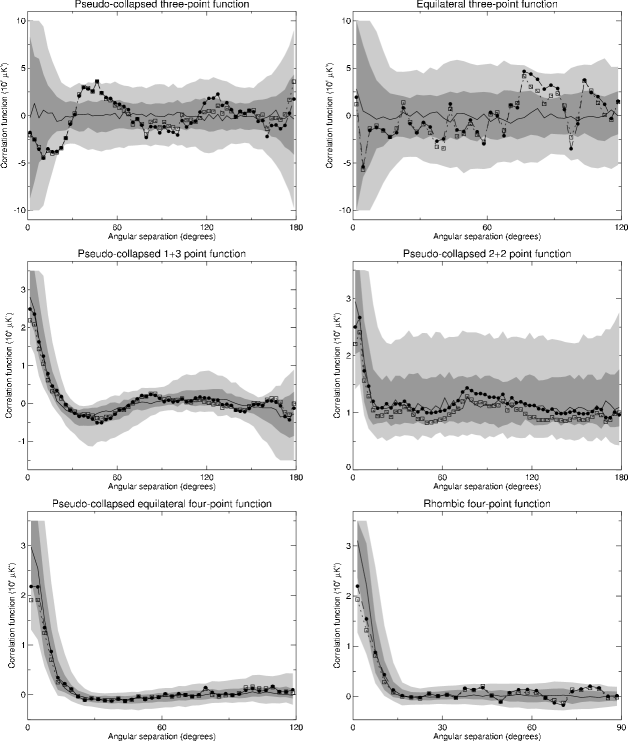
Figure 1: Three- and four-point correlation functions of the co-added 4-year DMR map. Solid line shows the most likely value for each bin, dark shading shows the 68% confidence region and light shading the 95% confidence region, as computed by Monte Carlo-simulations. Dots represent functions for the uncorrected co-added map, and boxes shows the functions for the map for which high-latitude Galactic emission has been removed. Note the different angular units on the horizontal axis, reflecting the fact that the various functions are defined on different angular intervals.

We also introduce one further small change compared to Hinshaw et al. (hinshaw (1995)) in that we exclude the zeroth angular bin (for which all $N$ pixels coincide) as any cosmological information here is heavily suppressed due to the low signal-to-noise ratio. Indeed, the inclusion of the zeroth bin only acts to increase the variance of the $\chi^{2}$ statistic, and is therefore better omitted.

3 Measurements of the COBE-DMR correlation functions

The COBE-DMR experiment resulted in six independent maps, two for each of the three frequencies at 31.5, 53 and 90 GHz. In this work we only include the maps from the 53 and 90 GHz channels, as they are superior in terms of the signal-to-noise ratio. The maps are analyzed in the HEALPix pixelization scheme, with a resolution parameter of $N_{\mathrm{side}}=32$, corresponding to 12 288 pixels on the sky. At each frequency we compute the ‘sum’ $(A+B)/2$ and ‘difference’ $(A-B)/2$ combinations, which yield, respectively, maps with enhanced signal-to-noise or noise content alone. In addition, we also generate a co-added map from the four basic channels using weights to achieve the optimal signal-to-noise ratio.

The two-, three- and four-point correlation functions for these nine map combinations are then computed. All pixels corresponding to the extended Galactic cut (Banday et al. banday (1997) but recomputed explicitly for the HEALPix scheme) are rejected from the analysis, leaving a total of 7880 accepted pixels. The best-fitting monopole, dipole and quadrupole are subtracted from each map before the $N$-point functions are evaluated. The observed correlation functions are also computed after correction for the diffuse foreground emission at high Galactic latitude, using information from the (appropriately scaled) DIRBE $140\ \mu\mathrm{m}$ map (Górski et al. gorski (1996)).

For our Monte Carlo ensemble, we simulate 10 000 individual realizations of the CMB sky, based on an a priori best-fit cosmological power spectrum. In particular, we consider scale-invariant Gaussian temperature fluctuations ($P(k)\propto Q_{\mathrm{rms-PS}}^{2}k^{n}$ with $n=1$) with $Q_{\mathrm{rms-PS}}=18\ \mu\mathrm{K}$, (Górski et al. gorski (1996)). The power-spectrum is filtered through the DMR beam and pixel window functions. To each simulated CMB sky, we add four noise realizations based on the rms noise levels and observation patterns of the observed 53 and 90 GHz sky maps. These are then combined to generate the corresponding sum, difference and co-added sky maps. These are then processed in an identical fashion to the DMR data.

We note that we have also assumed that there are no significant pixel-pixel noise correlations, although some will indeed be present as a consequence of the differential nature of the radiometers which couple observations separated by $\sim 60\degr$ on the sky. Lineweaver et al. (lineweaver94 (1994)) have investigated this effect in detail, and find a small excess signal is present in the 2-point correlation function at $60\degr$ for maps containing noise signal alone. However, we do not expect our results to be compromised by this assumption.

Fig. 1 shows the results from these calculations for the co-added maps. The observed functions lie comfortably within the confidence region defined by the Monte Carlo-simulations and there are no striking deviations visible by simple inspection.

4 The $\chi^{2}$ statistic

In order to quantitatively measure the agreement between the DMR maps and the simulated ensemble, we utilize the same $\chi^{2}$ methodology described by Kogut et al. (kogut (1996)):

$$\chi^{2}=\sum_{\alpha\beta}(D_{\alpha}-\bigl{<}S_{\alpha}\bigr{>})(\mathbf{M}^{-1})_{\alpha\beta}(D_{\beta}-\bigl{<}S_{\beta}\bigr{>})$$ (3)

Here $\alpha$ and $\beta$ denote angular bins, $D$ the DMR correlation function, and $\bigl{<}S_{\alpha}\bigr{>}$ the mean function computed from simulations. $\mathbf{M}$ is the binned covariance matrix:

$$\mathbf{M}_{\alpha\beta}=\frac{1}{N}\sum_{i}(S^{i}_{\alpha}-\bigr{<}S_{\alpha}\bigl{>})(S^{i}_{\beta}-\bigl{<}S_{\beta}\bigr{>})$$ (4)

The probability density function of this $\chi^{2}$ statistic is established by computing the same statistic for all maps in the ensemble, (ie. by substituting $D$ with each of the simulated maps, $S^{i}$). The resulting histogram represents the probability distribution function against which we compare the values from the DMR maps. Table 1 records the fraction of simulated maps with higher $\chi^{2}$ values than the observed DMR map. Thus, values of order 0.01 or 0.99 can be considered suspicious, while anything from 0.05 to 0.95 is acceptable.

		53 GHz maps				90 GHz maps
		$A$	$B$	$\frac{\mathrm{A+B}}{2}$	$\frac{\mathrm{A-B}}{2}$	$A$	$B$	$\frac{\mathrm{A+B}}{2}$	$\frac{\mathrm{A-B}}{2}$	Co-added
	Two-point	0.48	0.22	0.37	0.32	0.05	0.48	0.67	0.02	0.63
	Pseudo-collapsed three-point	0.13	0.33	0.65	0.42	0.51	0.05	0.43	0.27	0.59
	Equilateral three-point	0.20	0.84	0.29	0.65	0.76	0.95	0.92	0.49	0.67
	Pseudo-collapsed 1+3 point	0.64	0.59	0.62	0.17	0.78	0.83	0.85	0.53	0.81
	Pseudo-collapsed 2+2 point	0.47	0.62	0.61	0.96	0.29	0.34	0.94	0.16	0.79
Uncorrected	Pseudo-collapsed equilateral four-point	0.36	0.71	0.70	0.79	0.95	0.61	0.57	0.33	0.92
	Rhombic four-point	0.58	0.99	0.50	0.17	0.49	0.96	0.76	0.10	0.80
	All functions combined	0.34	0.56	0.43	0.45	0.45	0.28	0.79	0.05	0.75
	Two-point	0.52	0.25	0.36	0.32	0.05	0.49	0.63	0.02	0.60
	Pseudo-collapsed three-point	0.19	0.41	0.83	0.42	0.64	0.09	0.53	0.27	0.74
	Equilateral three-point	0.34	0.80	0.43	0.65	0.82	0.97	0.93	0.49	0.84
	Pseudo-collapsed 1+3 point	0.67	0.63	0.65	0.17	0.81	0.88	0.65	0.53	0.82
	Pseudo-collapsed 2+2 point	0.55	0.50	0.62	0.96	0.41	0.40	0.95	0.16	0.79
Corrected	Pseudo-collapsed equilateral four-point	0.49	0.77	0.83	0.79	0.97	0.78	0.74	0.33	0.95
	Rhombic four-point	0.53	0.99	0.52	0.17	0.58	0.96	0.78	0.10	0.88
	All functions combined	0.45	0.59	0.54	0.45	0.58	0.39	0.80	0.05	0.70

Table 1: Results from $\chi^{2}$ tests. The numbers indicate the fraction of simulated realizations with $\chi^{2}$ value higher than for the respective COBE map. The lower half shows the results for the DMR maps after correction for high latitude Galactic emission. The upper half shows the results for the uncorrected maps. The effect of Galactic emission appears to be minimal: this is not unexpected since a best-fit quadrupole has been removed from the data before analysis, and the Galactic emission is dominated by such large-scale structure.

In Kogut et al. (kogut (1996)) the results for the pseudo-collapsed and the equilateral three-point functions are given for the 53 GHz $(A+B)/2$ map; they find the fractions to be respectively 0.66 and 0.31, while we find 0.65 and 0.29. Considering the minor changes in the definitions of the correlation functions and the different pixelizations used, the agreement is most satisfactory.

Overall, the numbers indicate that the COBE-DMR maps agree very well with the simulations. The optimal co-added map, for which the signal-to-noise ratio is the highest, returns results comfortably in the accepted range, as does the combined analysis of all $N$-point functions. We conclude that the DMR maps are compatible with the Gaussian hypothesis as measured by this test.

5 Reducing four-point functions into two-point functions

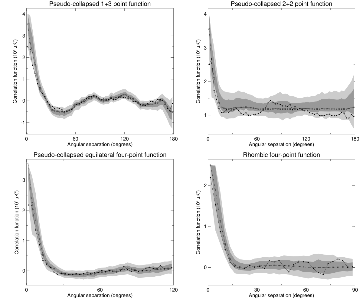
Figure 2: Comparison of the observed and the “reduced” four-point functions for the co-added DMR sky map. Boxes indicate the function predicted by the two-point functions, while shaded areas represent the 68% and 95% confidence intervals computed from Monte Carlo-simulations. The observed four-point functions are shown with a solid line.

Since it may be noted that all even-ordered $N$-point functions have non-vanishing expectation values determined by the two-point function, we can define an additional test of Gaussianity for the four-point functions. Explicitly, we take advantage of the following property (as, for example, described in Adler adler (1981)): If $Y_{1},Y_{2},\ldots,Y_{n}$ is a set of real-valued random variables having a joint Gaussian distribution and zero means, then for any integer $m$:

$$\bigl{<}Y_{1}Y_{2}\cdots Y_{2m+1}\bigr{>}=0$$ (5)

$$\bigl{<}Y_{1}Y_{2}\cdots Y_{2m}\bigr{>}=\sum\bigl{<}Y_{i_{1}}Y_{i_{2}}\bigr{>}\cdots\bigl{<}Y_{i_{2m-1}}Y_{i_{2m}}\bigr{>}$$ (6)

Here the sum goes over all $(2m-1)!!$ different ways of grouping $Y_{1},Y_{2},\ldots,Y_{2m}$ into $m$ pairs.

Thus, if the CMB temperature anisotropy field is in fact Gaussian distributed with zero mean, then all even $N$-point functions can be reduced to combinations of products of the two-point function. In particular, the four-point function reduces to:

$$\begin{split}\bigl{<}T_{1}T_{2}T_{3}T_{4}\bigr{>}=&\>\>\>\>\>\bigl{<}T_{1}T_{2}\bigr{>}\bigl{<}T_{3}T_{4}\bigr{>}\\ &+\bigl{<}T_{1}T_{3}\bigr{>}\bigl{<}T_{2}T_{4}\bigr{>}\\ &+\bigl{<}T_{1}T_{4}\bigr{>}\bigl{<}T_{2}T_{3}\bigr{>}\end{split}$$ (7)

For the four functions we defined in Sect. 2, we find the following expressions:

$$C^{1+3}(\theta) =3\>C_{2}(0)\>C_{2}(\theta)$$ (8)

$$C^{2+2}(\theta) =C_{2}(0)^{2}+2\>C_{2}(\theta)^{2}$$ (9)

$$C^{\mathrm{equi}}(\theta) =C_{2}(0)\>C_{2}(\theta)+2\>C_{2}(\theta)^{2}$$ (10)

$$C^{\mathrm{rhomb}}(\theta) =C_{2}(\theta)\>C_{2}(\theta^{\prime})+2\>C_{2}(\theta)^{2}$$ (11)

In equation (11) $\theta^{\prime}$ denotes the length of the longest axis of the rhombus, which is easily computed by spherical trigonometry:

$$\cos\frac{\theta^{\prime}}{2}=\frac{\cos\theta}{\cos\frac{\theta}{2}}$$ (12)

Note that the functions given by Eqs. (8)-(11) should be interpreted as expectation values. That is, the observed four-point function should equal that given by Eq. (7) to the same extent that the three-point function equals zero. Thus, to establish an acceptable distribution for these relations we again utilize our Monte-Carlo simulation set. We compare the simulated ensemble of functions to those predicted by Eqs. (8)–(11): for each realization in the ensemble, we compute the four-point function predicted by the two-point function relation above, and then evaluate the difference between this predicted and the observed four-point function. From these differences we generate 68% and 95% confidence intervals. Finally, the procedure is repeated for the DMR maps, and the results are compared to the derived confidence intervals.

This procedure has one major advantage compared to the one described in Sect. 3: the power spectrum only mildly affects the result. That is, the two most important contributions to the analysis come from the map itself, in the form of a two-point and a four-point function. The assumed power spectrum is only used for estimating the acceptable deviations, not the overall shape. Therefore, this procedure provides a more direct test for Gaussianity than the previous one.

		53 GHz maps				90 GHz maps
		$A$	$B$	$\frac{\mathrm{A+B}}{2}$	$\frac{\mathrm{A-B}}{2}$	$A$	$B$	$\frac{\mathrm{A+B}}{2}$	$\frac{\mathrm{A-B}}{2}$	Co-added
	Pseudo-collapsed 1+3 point	0.73	0.69	0.32	0.17	0.81	0.51	0.87	0.52	0.60
	Pseudo-collapsed 2+2 point	0.46	0.62	0.58	0.95	0.27	0.32	0.90	0.14	0.75
	Pseudo-collapsed equilateral four-point	0.40	0.62	0.54	0.79	0.92	0.61	0.57	0.31	0.79
Uncorrected	Rhombic four-point	0.49	0.98	0.60	0.17	0.50	0.94	0.75	0.09	0.76
	Pseudo-collapsed 1+3 point	0.87	0.76	0.35	0.17	0.86	0.61	0.81	0.52	0.71
	Pseudo-collapsed 2+2 point	0.52	0.52	0.58	0.95	0.39	0.38	0.92	0.14	0.73
	Pseudo-collapsed equilateral four-point	0.54	0.71	0.69	0.79	0.94	0.79	0.74	0.31	0.81
Corrected	Rhombic four-point	0.50	0.98	0.67	0.17	0.58	0.94	0.80	0.09	0.87

Table 2: Results for the modified $\chi^{2}$ statistic. The numbers refer to the fraction of simulations with $\chi^{2}$ values higher than the corresponding COBE-DMR maps. The upper half shows the results for the uncorrected maps, while Galactic emission has been corrected for in the lower half.

The results are shown for the co-added map in Fig. 2. The observed function lies well within the confidence regions about the predicted function for all four cases. For a more quantitative measure of the perceived agreement, we define a $\chi^{2}$ statistic, incorporating the new degree of freedom provided by the predicted four-point function by simply replacing the average correlation function with that new function:

$$\chi^{2}=\sum_{\alpha\beta}(D_{\alpha}-D_{\alpha}^{\mathrm{pred}})(\mathbf{M}^{-1})_{\alpha\beta}(D_{\beta}-D_{\beta}^{\mathrm{pred}})$$ (13)

where

$$\mathbf{M}_{\alpha\beta}=\frac{1}{N}\sum_{i}(S^{i}_{\alpha}-S_{\alpha}^{i,\mathrm{pred}})(S^{i}_{\beta}-S_{\beta}^{i,\mathrm{pred}})$$ (14)

The meaning of each symbol is the same as in Eqs. (3) and (4).

Table 2 summarizes the results, which again support the hypothesis that the DMR sky maps are consistent with a scale-invariant cosmological model with Gaussian initial fluctuations.

6 Conclusions

By performing Monte Carlo-simulations we have studied the statistical properties of the COBE-DMR 53 GHz and 90 GHz channels. The basic ingredients for this analysis were various $N$-point correlation functions, and, in particular, four different four-point functions which have been presented for the first time. We have additionally taken advantage of a result from statistical theory, relating all even $N$-point functions to reductions in terms of the two-point function. This allowed us to define a test for Gaussianity in which the assumed power spectrum only plays a secondary role. This test could therefore prove better suited for situations in which we do not have access to the optimal power spectrum.

Comparison of the DMR $N$-point correlation functions with the Monte-Carlo ensemble indicates no evidence for possible non-Gaussian behavior, in agreement with the earlier analysis of Kogut et al. (kogut (1996)). Furthermore, the agreement between the observed DMR functions and the simulated ensembles also supports the validity of our model assumptions, namely that of a scale-invariant power law model for the anisotropies, and uncorrelated noise.

On the other hand, the excellent agreement between the simulated and the observed correlation functions poses an intriguing problem: tests of Gaussianity based on a harmonic analysis of the DMR data – the bispectrum work of Ferreira et al. (ferreira (1998)) and trispectrum results of Kunz et al. (kunz (2001)) – show compelling evidence for non-Gaussian features (although these have subsequently been associated with systematic artifacts in the DMR data by Banday et al. bandaya (2000)), while tests based on real-space high-order statistics such as those presented here do not. The resolution of such apparently contradictory results is most likely rather mundane: the source of the non-Gaussian signal was found to be strongly located at the multipole order $l=16$. Since the correlation functions are by definition (weighted) averages over the full multipole range, the reduced sensitivity to this type of non-Gaussian structure is certainly not unexpected.

- (1) Adler, R. J. 1981, The Geometry of Random Fields, John Wiley & Sons.
- (2) Banday, A. J., Górski, K. M., Bennett, C. L., et al. 1997, ApJ, 475, 393
- (3) Banday, A. J., Zaroubi, S. & Górski, K. M. 2000, ApJ, 533, 575
- (4) Barreiro, R. B., Hobson, M. P., Lasenby, A. N., et al. 2000, MNRAS, 318, 475B
- (5) Cayón, L., Sanz, J. L., Martínez-González, E., et al. 2001, MNRAS, 326, 1243C
- (6) Ferreira, P. G., Magueijo, J. & Górski, K. M. 1998, ApJ, 503, L1
- (7) Górski, A., Banday, A. J., Bennett, C. L., et al. 1996, ApJ, 464, L11
- (8) Hinshaw, G., Banday, A. J., Bennett, C. L., Górski, K. M. & Kogut, A. 1995, ApJ, 446, L67
- (9) Kogut, A., Banday, A. J., Bennett, C. L., et al. 1996, ApJ, 464, L29
- (10) Komatsu, E., Wandelt, B. D., Spergel, D. N., Banday, A. J. & Górski, K. M. 2002, ApJ, 566, 19K
- (11) Kunz, M., Banday, A. J., Castro, P. G., Ferreira, P. G. & Górski, K. M. 2001, ApJ, 563, L99
- (12) Lineweaver, C. H., Smoot, G. F., Bennett, C. L., et al. 1994, ApJ, 436, 452
- (13) Magueijo, J. 2000, ApJ, 528L, 57M
- (14) Novikov, D., Schmalzing, J. & Mukhanov, V. F. 2000, A&A, 364, 17N
- (15) Sandvik, H. B. & Magueijo, J. 2001, MNRAS, 325, 463S
- (16) Schmalzing, J., & Górski, K. M., 1998, MNRAS, 297, 355