A feature at $z\sim 3.2$ in the evolution of the Ly$\alpha$ forest optical depth

Abstract

The effective optical depth in the Ly$\alpha$ forest region of 1061 low-resolution QSO spectra drawn from the SDSS database decreases with decreasing redshift over the range $2.5\leq z\leq 4$. Although the evolution is relatively smooth, $\tau_{\rm eff}\propto(1+z)^{3.8\pm 0.2}$, at $z\sim 3.2$ the effective optical depth decreases suddenly, by about ten percent with respect to this smoother evolution. It climbs back to the original smooth scaling again by $z\sim 2.9$. We describe two techniques, one of which is new, for quantifying this evolution which give consistent results. A variety of tests show that the feature is not likely to be a consequence of how the QSO sample was selected, nor the result of flux calibration or other systematic effects. Other authors have argued that, at this same epoch, the temperature of the IGM also shows a departure from an otherwise smooth decrease with time. These features in the evolution of the temperature and the optical depth are signatures of the reionization of He II.

1 Introduction

The importance of resonant scattering by neutral hydrogen in the intergalactic medium (IGM) was described by Gunn & Peterson (1965), who used the lack of a strong absorption trough in the spectra of high-redshift quasars to set limits on the amount of dispersed H I. Lynds (1971) noted that in the spectra of distant quasars there are many absorption features blueward of the Ly$\alpha$ emission line; he interpreted the absorption features as Ly$\alpha$ lines produced by intervening material. The mean absorption in the Ly$\alpha$ forest depends mainly on the gas density and the amplitude of the ionising background (Rauch et al. 1997; Rauch 1998). The absorption increases rapidly with increasing redshift $z$ (e.g., Schneider, Schmidt & Gunn 1991; Songaila & Cowie 2002).

The optical depth $\tau$ for a gas consisting primarily of ionized hydrogen and singly ionized helium, which is at density $(1+\delta)\equiv\rho/\langle\rho\rangle$ relative to the background density $\langle\rho\rangle$ and is in photo-ionization equilibrium at redshift $z$, is

$$\tau(z)\approx 0.7\,\left({\Omega_{b}h^{2}\over 0.019}\right)^{2}\,\left({\Omega_{m}h^{2}\over 0.3\times 0.65^{2}}\right)^{-1/2}\,\left({1+z\over 4}\right)^{4.5}\,{T_{4}^{-0.7}\over\Gamma_{12}}\,{(1-Y)\over 0.76}{(1-Y/4)\over 0.94}\,(1+\delta)^{2}$$ (1)

where $\Omega_{b}h^{2}$ is the baryon density, $H_{0}=100h$ km s^-1 Mpc^-1 is Hubble’s constant, $\Omega_{m}$ is the matter density, and $Y$ is the helium abundance by mass (e.g. Peebles 1993, §23). The temperature of the gas is $T_{4}\equiv T/10^{4}K$, and $\Gamma_{12}\equiv\Gamma/10^{-12}$ s^-1 is the photo-ionization rate. Equation (1) suggests that $\tau$ should evolve rapidly. Various authors (e.g., Jenkins & Ostriker 1991; Hernquist et al. 1996; Rauch et al. 1997) have noted that measurements of the mean transmission $\langle{\rm exp}(-\tau)\rangle$ and its evolution constrain the parameters in equation (1), such as the ratio $(\Omega_{b}h^{2})^{2}/(\Omega_{m}h^{2})^{1/2}$ (Rauch 1998), and the evolution of $T_{4}^{-0.7}/\Gamma_{12}$ (McDonald & Miralda-Escudé 2001).

Equation (1) shows that, after the reionization of H I, the optical depth is expected to decrease smoothly with time, unless, for example, there is a sudden injection of energy into the IGM. For instance, if the temperature of the gas increases by a factor of two at some epoch, then equation (1) suggests that the optical depth $\tau$ in the Ly$\alpha$ forest would decrease by a factor of $2^{-0.7}\sim 0.6$. There is some evidence of a factor of two change in the temperature of the IGM at $z\sim 3-3.5$ (e.g. Schaye et al. 2001).

Reimers et al. (1997; also see Heap et al. 2000; Kriss et al. 2001) found evidence for a sharp increase in the He II opacity around $z\sim 3$, which they associated with He II reionization. Songaila & Cowie (1996) and Songaila (1998) have argued that the observed evolution of C IV/Si IVmetal line ratios requires a sudden hardening of the ionizing background around $z\sim 3$, which is consistent with He II reionization. Schaye et al. (2000) and Theuns et al. (2002a,b) showed that He II reionization at $z\sim 3.5$ results in a jump of about a factor of two in the temperature of the IGM at the mean density, and found evidence for such a jump by studying the distribution of line-widths in the Ly$\alpha$ forest. In addition, Schaye et al. (2000) and Ricotti, Gnedin & Shull (2000) found that the gas is close to isothermal at redshift $z\sim 3$, indicating that a second reheating of the intergalactic medium took place at $z\sim 3$. This too might be interpreted as evidence of the reionization of He II. (Numerical simulations of the observational signatures of He II ionization are also presented in e.g., Meiksin 1994 and Croft et al. 1997.) However, Boxenberg (1998) and Kim, Cristiani, & D’Odorico (2002) found no change in C IV/Si IV, and analyses by McDonald et al. (2001) and Zaldarriaga, Hui, & Tegmark (2001) did not find a significant temperature change at these redshifts. Thus, both from metal line ratios, and from measurements of line widths, there is some evidence for He II reionization at $z\sim 3-3.5$, and that this event is associated with an increase in the temperature of the IGM, although the strength of the evidence is still being questioned.

If He II were ionized at $z\sim 3-3.5$, and this caused the temperature of the IGM to increase by a factor of two, then our simple estimate of an associated sixty percent decrease in $\tau$ is not quite right. For instance, it ignores the fact that the extra electron liberated by the ionization can increase the optical depth. However, for $Y\sim 0.24$, the increase in the electron density from the electron released by He II ionization can increase $\tau$ only by seven or eight percent. Although this goes in the opposite direction to the effect of the temperature increase, it is a substantially smaller effect. Other important factors, which the simple sixty-percent estimate ignores, include the facts that the temperature change may be accompanied by a change in the temperature–density relation of the gas; that saturated lines which contribute to the optical depth will not be as strongly affected by a temperature change; and that a temperature increase may expand the gas, thus affecting peculiar velocities and complicating the relationship between temperature, line profile and optical depth. Nevertheless, the discussion above indicates that a sudden change in the temperature of the IGM may well be accompanied by a sudden change in the optical depth, although a precise estimate of the magnitude of the effect requires hydrodynamical simulations.

A sudden change in $\tau$ means that the ratio of the mean absorption in the Ly$\alpha$ forest to that in the spectrum of the quasar (hereafter QSO) should also change abruptly at the same time. That is, the quantity defined by Oke & Korycansky (1982),

$$D_{A}\equiv 1-\bar{F},\qquad{\rm where}\qquad\bar{F}\equiv{F_{\lambda}({\rm observed})\over F_{\lambda}({\rm continuum})}\equiv\exp(-\tau_{\rm eff})$$ (2)

should show a feature at $z\sim 3-3.5$ if He II was ionized at that time. An advantage of studying the mean absorption, $D_{A}$, or transmission, $\bar{F}$, is that it can be measured even in low resolution spectra for which individual line measurements are not possible. It is conventional to use the mean transmission to define an effective optical depth: $\tau_{\rm eff}\equiv-\ln\bar{F}$. Schneider, Schmidt & Gunn (1991) show that the mean transmission evolves significantly over the range $0<z<4.5$ (also see Press, Rybicki & Schneider 1993). The main goal of this paper is to see if this evolution is smooth, or has a feature in it. For example, we would like to see if there is any evidence of a sudden drop in the effective optical depth in the Ly$\alpha$ forest at $z\sim 3-3.5$.

Section 2 describes how we selected our sample of $\sim 10^{3}$ QSOs from the Sloan Digital Sky Survey (SDSS) database. The SDSS QSO selection algorithm itself is studied in some detail in Appendix B. We will be searching for a feature in the evolution of the mean transmission; this requires an accurate determination of the underlying intrinsic QSO spectrum. This is the subject of Section 3. We use two methods to do this. one method, which is a direct descendent of the one first used by Oke & Korycansky (1982), is described in Appendix A. The other is new; it exploits the fact that the continuum is a function of restframe wavelength, whereas the Ly$\alpha$ effective optical depth is a function of observed wavelength. Both methods yield consistent results—the inferred continuum between the Ly$\alpha$ and Ly$\beta$ emission lines is not featureless, and, at $z\sim 2.9-3.3$, there appears to be a feature in the otherwise smooth evolution of the mean transmission, and hence of $\tau_{\rm eff}$. Possible systematic effects which might affect our measurement are discussed in Section 4 and in Appendix B. A final section summarizes our findings. Appendix C is somewhat tangential to the main subject of this paper: it is a short demonstration of some effects which arise from the fact that the distribution of flux decrements in the Ly$\alpha$ forest is highly non-Gaussian.

A comparison of this measurement with predictions from hydrodynamical simulations shows that our measurements can be interpreted as evidence for He II reionization at $z\sim 3.2$ (Theuns et al. 2002). The implications for the evolution of the temperature of the IGM and the photo-ionization rate $\Gamma$ will be presented in a future paper.

2 Sample selection

The sample of QSOs used in this paper was extracted from the SDSS database (York et al. 2000) which included all the spectra observed by the SDSS collaboration through the end of 2001. This sample is about three times larger than that in the SDSS Early Data Release (Stoughton et al. 2002). The SDSS camera is described in Gunn et al. 1998, and the filter response curves are described in Fukugita et al. (1996). The SDSS photometric reduction procedure is described in Lupton et al. (2000), and the spectroscopic data reduction procedure will be described in Frieman et al. (2002). The SDSS procedure for targeting QSOs is described in detail in Richards et al. (2002a).

Figure 1: Examples of QSO spectra in our sample, shown here as a function of wavelength in the restframe. Dashed line shows a power-law in wavelength of slope $\alpha_{\lambda}=-1.56$, normalized to have the same flux as the observed spectra in the rest wavelength range $1450-1470$ Å. Solid line shows the continuum obtained as described in Section 3. We analyse the Ly$\alpha$ forest in the wavelength region 1060–1180 Å.

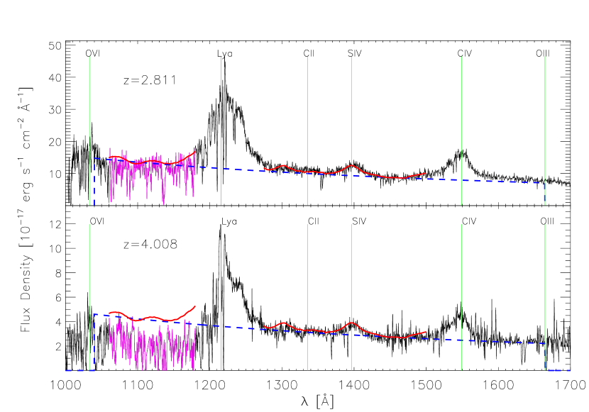
When we selected our sample, the SDSS had imaged $\sim 4000$ square degrees, and $\sim 20,000$ QSOs had both photometric and spectroscopic information. The SDSS spectroscopic pipeline identifies any extragalactic object whose spectrum is dominated by a non-stellar continuum and has at least one broad emission line (rest-frame FWHM larger than $1000$ kms^-1) as a candidate QSO (Frieman et al. 2002). Thus, the sample of $\sim 20,000$ objects includes Seyfert galaxies and some “Type 2” AGNs as well as QSOs. All of these spectra were examined visually to make certain that the redshift was correctly assigned. Spectra with broad absorption line features (BAL QSOs) for which it was not possible to measure a redshift are not included in the above.

We are interested in compiling a sample of objects in which the Ly$\alpha$ forest can be easily detected. The requirement that the entire forest (restframe wavelength $\sim 1050-1180$ Å) be detected in the SDSS spectrum of an object sets a lower limit of $z\approx 2.75$ on the redshift of the QSOs we will analyze. In turn, this sets a limit of about $z_{\alpha}\geq 2.5$ on the redshift range in which we can study the Ly-$\alpha$ forest. In practice, there is a problem with the flux calibration of the SDSS spectra at the blue end of the spectrograph (wavelengths shorter than 4400Å, see Appendix B.2. Therefore, we only show results at slightly higher redshifts, which are not affected by this. Of the $\sim 20,000$ QSO–candidate objects above, about $1400$ are at $z\geq 2.75$. About 250 of these had spectra with unusually broad absorption lines (BALs), or strong damped Ly$\alpha$ systems, and/or had low quality spectra, so we removed them from our sample.

The instrumental resolution of the SDSS spectrograph is about $150$ kms^-1. Studies of higher resolution QSO spectra show that most lines in the Ly$\alpha$ forest are substantially narrower than this. Therefore, a typical line in the Ly$\alpha$ forest is unresolved in our data. In addition, the SDSS QSO spectra have a median $S/N$ per pixel of $\sim 10$, and this ratio drops to $\sim 3$ in the Ly$\alpha$ forest. Therefore, for the SDSS sample, measuring the parameters of individual Ly$\alpha$ lines as a function of redshift is not the best way to estimate the temperature evolution of the IGM. A better approach is to measure the mean transmission of the flux in the Ly$\alpha$ forest, $\bar{F}$, as a function of redshift. Equation (2) shows that the crucial step is to determine the QSO continuum precisely. To do so, we must have a reasonably long restframe wavelength range which is common to all the objects in our sample—we require that the restframe range $1250-1665$ Å be detected in all the spectra we will include in our sample. This sets an upper limit $z\approx 4.3$ on the redshifts of the objects we will include in our analysis. This requirement removed an additional $\sim 100$ objects, leaving 1061 QSO spectra in our sample; two examples are shown in Figure 1.

3 Estimating the continuum and the mean transmission

In what follows, it will be useful to think of the observed flux in the spectrum of the $i$th QSO (shifted to the restframe of the QSO and normalized in some standard fashion which we will discuss shortly) as

$$f_{i}(\lambda_{rest})=\Bigl{[}C(\lambda_{rest}|z_{i})+c_{i}(\lambda_{rest})\Bigr{]}\,\Bigl{[}T(z_{\alpha})+\ t_{i}(z_{\alpha})\Bigr{]}+n_{i}(\lambda_{obs}),\qquad{\rm where}\qquad 1+z_{\alpha}\equiv{\lambda_{obs}\over\lambda_{\alpha}}={\lambda_{rest}(1+z_{i})\over 1215.67},$$

$z_{i}$ is the redshift of the QSO and $\lambda_{\alpha}\equiv 1215.67$ Å. Here $C$ represents the mean continuum at fixed rest wavelength, which we think of as being representative of the QSO population at $z_{i}$ as a whole (if QSOs evolve, then the mean continuum of the population may depend on redshift), and $c_{i}$ represents the fact that the continuum of the $i$th QSO might be different from the mean at that redshift. ($c_{i}$ could also differ from one QSO to another if relativistic outflows from QSOs are common. See Richards et al. 1999 and references therein for evidence of such relativistic velocities.) Similarly, $T(z_{\alpha})\equiv\exp[-\tau_{\rm eff}(z_{\alpha})]$ is the mean transmission through the Ly$\alpha$ forest at $z_{\alpha}$, averaged over all the $z_{\alpha}$ pixels in the forest (note that $\tau_{\rm eff}$ is a function of $z_{\alpha}$, and hence of the observed rather than restframe wavelength), and $t_{i}$ represents the fact that the transmission through the forest along the $i$th line of sight might be different from the mean value. The final term $n_{i}$ represents the noise in the observation. By definition $\langle c_{i}\rangle\equiv 0$ and $\langle t_{i}\rangle\equiv 0$, where the average over $c_{i}$ is over fixed $\lambda_{rest}$, and the average of $t_{i}$ is over fixed $z_{\alpha}$, and hence over fixed $\lambda_{obs}$. We will assume that, at fixed $\lambda_{obs}$, $\langle n_{i}\rangle=0$ also. We have written the observed flux in this way to emphasize the fact that the mean continuum $C$ is a function of $\lambda_{rest}$, whereas the mean transmission $T=\exp(-\tau_{\rm eff})$ is a function of $\lambda_{obs}$. It is this fact which makes it possible, at least in principle, to disentangle the two unknown functions $C$ and $T$ from the single observed quantity, $f$.

All work to date first estimates $C+c_{i}$, and then averages all the $f_{i}/(C+c_{i})$ which have the same $z_{\alpha}$ to estimate the mean transmission. That is, the shape of the continuum is determined separately for each QSO. This is easier to do at low redshifts $z\leq 1$ where absorption by the forest is smaller, but it is considerably more difficult at higher redshifts. Furthermore, if the resolution of the spectrograph is low and/or the signal-to-noise ratio is poor, then systematic errors in the estimated continuum can arise (Steidel & Sargent 1987). Biases can also arise if some fraction of the absorption is not due to H I but to other elements. This extra absorption becomes increasingly important at lower redshifts, as the Ly$\alpha$ opacity decreases more rapidly than the opacity of the metals. For example, at $z\sim 2.5$, approximately 20% of the total absorption in the Ly$\alpha$ forest is not due to H I (Kulkarni et al. 1996; Rauch 1998). Our sample is confined to high enough redshifts that this should not be a significant concern, although, as we discuss later, absorption by elements other than H I may be important when comparing our measurements to results from higher resolution spectra.

Our spectra have low resolution and signal-to-noise, so an object-by-object estimate of the continuum is difficult. On the other hand, our sample is very large, so we can take a statistical approach. Consider QSOs in a small redshift range. The QSOs have a range of luminosities, and so the set of spectra in any one redshift bin can differ considerably from each other. When suitably normalized, however, the differences between spectra are reduced significantly. Therefore, following Press, Rybicki & Schneider (1993) and Zheng et al. (1997), we normalize each spectrum by the flux in the rest wavelength range $1450-1470$ Å. (This wavelength range lies in front of the C IV emission line, and is free of obvious emission and absorption lines.) Having normalized each observed spectrum we compute the average value of the normalized flux $f_{i}$ to obtain a composite spectrum. This composite is

$$\langle f_{i}\rangle=CT+\langle Ct_{i}\rangle+\langle c_{i}T\rangle+\langle c_{i}t_{i}\rangle+\langle n_{i}\rangle=CT,$$

where we have assumed that the averages $\langle Ct_{i}\rangle$, $\langle c_{i}T\rangle$, $\langle c_{i}t_{i}\rangle$ and $\langle n_{i}\rangle$, evaluated at fixed $\lambda_{rest}$ and QSO redshift are all zero. For a sufficiently large sample, these averages probably are vanishingly small, so we can interpret the measured composite spectrum as the product of the mean continuum times the desired mean transmission. Because $\langle f_{i}/C\rangle=\langle f_{i}/(C+c_{i})(1+c_{i}/C)\rangle=\langle f_{i}/(C+c_{i})\rangle+\langle f_{i}/(C+c_{i})(c_{i}/C)\rangle$, this estimate of the mean transmission differs from the usual one by the second term: $\langle f_{i}/(C+c_{i})(c_{i}/C)\rangle$. If the transmission $f_{i}/(C+c_{i})$ in the $i$th spectrum is not correlated with how different the continuum of the $i$th QSO is compared to the average continuum, $c_{i}/C$, then this second term can be written as two separate averages. In this case, $\langle f_{i}/C\rangle=\langle f_{i}/(C+c_{i})\rangle$ because $\langle c_{i}/C\rangle\equiv 0$.

Figure 2: First four components (or eigen-spectra) obtained from a principle component analysis (PCA) of all the QSO spectra in the redshift bin $2.9<z<3.3$. Eigen-spectra for the other redshift bins are similar. The second and higher order components mainly try to fit the emission line features accurately; the overall shape is determined primarily by the first component.

If QSOs at the same redshift have a wide variety of spectra, then the composite spectrum could be very different from the spectrum of any individual object, thus making our estimates of the mean transmission blueward of $\lambda_{\alpha}$ very noisy. Therefore, we carried out a principle component analysis (PCA; e.g., Francis et al. 1992) of the spectra in the wavelength range $1200-1665$ Å. Figure 2 shows the first four components (or eigen-spectra) determined by the PCA for the QSOs in the redshift range $2.9<z<3.3$ (the other redshift bins show similar eigen-spectra). The first component (upper left panel) represents the intervals $1280-1500$ Å and $1580-1665$ Å well. The next $10-15$ components are mainly necessary for reproducing the exact shape of the Ly$\alpha$ and C IV emission lines. In particular, because the flux density of these higher order components is close to zero in the $1280-1500$ Å and $1580-1665$ Å wavelength regions, the PCA analysis suggests that, in these regions QSO spectra are very similar to each other. Therefore, our decision to combine all the QSOs at a given redshift when estimating the shape of the continuum (i.e., to treat all QSOs at a given redshift as differing in the normalization, but not the shape, of the continuum) is likely to be reasonable.

Figure 3: Composite restframe spectra (i.e. wavelengths have been transformed to the restframe of the QSO, and flux densities were normalized to sum to the same value in the range $1450-1470$ Å) in different redshift bins; curve which is highest at small $\lambda$ is for $2.95\leq z<3.15$, and bins in redshift step by $\Delta z=0.2$ down to the lowest curve which is for $4.15\leq z<4.3$. Redward of the Ly$\alpha$ emission line, the different composites are extremely similar. In contrast, the region blueward of $\lambda_{\alpha}=1215.67$ Å changes rapidly with redshift. The bumps at $\lambda=1070$ Å and $\lambda=1120$ Å are emission features intrinsic to the QSO spectrum. The vertical lines on the left show three different wavelength regions adopted in defining the Ly$\alpha$ forest: 1060–1180 Å (dashed), 1080-1160 Å (dot-dot-dot-dashed), and 1100–1150 Å (dot-dashed).

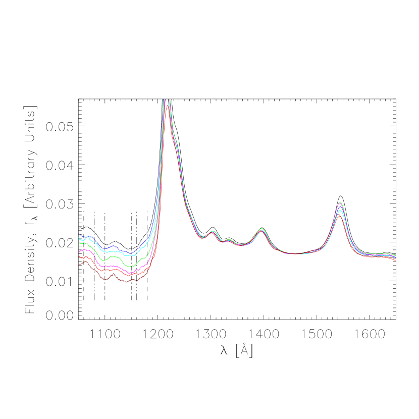
Figure 3 shows composite spectra as a function of restframe wavelength for a number of bins in redshift: the curve which is highest on the left is for $2.95\leq z<3.15$, the next highest is for $3.15\leq z<3.35$, and so on, until the lowest curve which is for $4.15\leq z<4.3$. The bins in $\lambda$ over which this averaging was done were chosen to be as small as possible—they were set by the SDSS pixel sizes. There are typically about 100 QSOs per bin (Figure 16 shows the exact distribution of QSO redshifts in our sample). The vertical lines on the left show three different wavelength regions adopted in defining the Ly$\alpha$ forest: 1060–1180 Å (dashed), 1080-1160 Å (dot-dot-dot-dashed), and 1100–1150 Å (dot-dashed).

Redward of the Ly$\alpha$ emission line at $\lambda_{\alpha}=1215.67$ Å, the different curves in Figure 3 are all very similar to each other (although the C IV emission line and redward may be evolving slightly, and the uppermost curve, corresponding to the QSOs in the lowest redshift bin, appears to be slightly different from all the others; the apparent evolution of the red wing of the C IV line is discussed in more detail by Richards et al. 2002b). Evidently, redward of $\lambda_{\alpha}$, the QSO population as a whole evolves little between $z\sim 4.3$ and $z\sim 3$. Blueward of $\lambda_{\alpha}$, however, there is an obvious trend: there is less observed flux in the spectra of higher redshift QSOs. Our problem is to turn this trend into a quantitative estimate of how the effective optical depth evolves. This can be done because the effective optical depth is the same at fixed observed, rather than restframe wavelength, whereas the continuum is a function of restframe wavelength.

To illustrate, consider the bumps at 1070 Å and 1120 Å. Because they are present at the same restframe wavelengths in all the redshift bins, they cannot have been caused by features in the evolution of the optical depth. (If we define the Ly$\alpha$ forest as spanning the range $1060-1180$ Å, then for the lowest redshift bin, $2.95\leq z<3.15$, the forest spans the range $2.44\leq z_{\alpha}<3.03$, whereas for the highest redshift bin, $4.15\leq z<4.3$, the forest spans $3.49\leq z_{\alpha}<4.14$. Features at fixed $z_{\alpha}$ would appear at quite different wavelengths for the different QSO redshift bins.) Therefore, the bumps must be intrinsic to the QSO spectrum—they could be Ar I and Fe III in emission. Their presence can affect our estimates of the effective optical depth in the forest.

In low resolution observations such as ours, the continuum level is usually calibrated redwards of the Ly$\alpha$ emission line and then extrapolated bluewards assuming a smooth power-law shape (e.g., Press, Rybicki & Schneider 1993). However, departures from a smooth power-law, such as the two emission lines at $\sim 1070$ Å and $\sim 1120$ Å, are clearly present in our data. (Figure 5 of Press, Rybicki & Schneider 1993 also shows bumps at these wavelengths, although they do not call attention to them.) In addition, at wavelengths close to the Ly$\alpha$ or Ly$\beta$/O VI emission features, emission from the QSO can contaminate the flux in the forest—smooth power-law fits to the mean continuum shape cannot account for this. The following section describes how we solve simultaneously for the evolution of the effective optical depth and for the shape of the mean continuum, while allowing for the possibility that neither are well-fit by featureless power-laws.

3.1 Method: A minimization approach

The observed composite spectrum is the product of the mean continuum times the mean transmission. This fact suggests defining

$$\chi^{2}=\sum_{i}\left(f_{i}(\lambda_{rest})-C(\lambda_{rest})\,{\rm e}^{-\tau_{\rm eff}(\lambda_{obs}/\lambda_{\alpha})}\,\right)^{2},$$ (3)

where the sum is over all pixels in all spectra in the sample which fall in the wavelength range associated with the forest. The composite spectra suggest that the continuum is the superposition of a power-law, two emission lines and the blueward side of the Ly$\alpha$ emission line. Therefore, we parametrize

$$C=c_{0}\,\left(\lambda_{rest}\over\lambda_{\alpha}\right)^{c_{1}}+c_{2}\,\exp\left(-{(\lambda_{rest}-c_{3})^{2}\over 2\,c_{4}^{2}}\right)+c_{5}\,\exp\left(-{(\lambda_{rest}-c_{6})^{2}\over 2\,c_{7}^{2}}\right)+c_{8}\,\exp\left(-{(\lambda_{rest}-c_{9})^{2}\over 2\,c_{10}^{2}}\right),$$

and we set

$$T=\exp(-\tau_{\rm eff})\qquad{\rm with}\qquad\tau_{\rm eff}=t_{0}\,\left({\lambda_{rest}(1+z_{i})\over\lambda_{\alpha}}\right)^{t_{1}}+t_{2}\,\exp\left(-{(\lambda_{rest}(1+z_{i})/\lambda_{\alpha}-t_{3})^{2}\over 2\,t_{4}^{2}}\right),$$

so as to allow the possibility of a feature centred at $1+z_{\alpha}=t_{3}$ superimposed on an otherwise smooth power-law evolution of $\tau_{\rm eff}$. To reduce the number of free parameters we have fixed the position of the peak of the Ly$\alpha$ emission line ($c_{9}=1215.67$ Å) and of the other two emission lines seen in the composite spectrum ($c_{3}=1073$ Å and $c_{6}=1123$ Å). Then the remaining eight parameters of $C$ and the five parameters of $\tau$ are varied until $\chi^{2}$ has been minimized (note that $\lambda_{\alpha}=1215.67$ is not a parameter). In principle, we could have attempted to fit the emission lines redward of $\lambda_{\alpha}$ (as was done by Press, Rybicki & Schneider 1993). Since we are more interested in the shape of the continuum blueward of $\lambda_{\alpha}$, we did not do this.

The exact parameter values which minimize $\chi^{2}$ depend somewhat on the range used to define the Ly$\alpha$ forest. We have tried three ranges which are shown in Figure 3: the largest range 1060–1180 Å (shown by the dashed lines) requires that we understand the continuum even in the regime which is close to the Ly$\alpha$ emission line, the shorter less demanding range 1080–1160 Å (dashed-dot-dot-dotted lines) is our standard, and the shortest, most conservative range is 1100–1150 Å (dashed-dotted lines).

Table 1: Values which minize $\chi^{2}$ as defined by equation (3). Two sets of values are shown: first is for the entire sample, second is for a subset which has a higher signal-to-noise ratio.

All		$c_{0}$	$c_{1}$	$c_{2}$	$c_{3}$	$c_{4}$	$c_{5}$	$c_{6}$	$c_{7}$	$c_{8}$	$c_{9}$	$c_{10}$
1061		0.0220	$-1.56$	0.0023	1073	11	0.0022	1123	13	0.025	1216	25
	$\pm$	$0.0006$	$\ \ 0.02$	$0.0003$	–	$1$	$0.0002$	–	$2$	$0.008$	–	$1$
				$t_{0}$	$t_{1}$	$t_{2}$	$t_{3}$	$t_{4}$
				0.0028	3.69	$-0.06$	4.15	0.08
			$\pm$	$0.0011$	$0.22$	$\ \ 0.02$	$0.02$	$0.02$
$S/N>4$		$c_{0}$	$c_{1}$	$c_{2}$	$c_{3}$	$c_{4}$	$c_{5}$	$c_{6}$	$c_{7}$	$c_{8}$	$c_{9}$	$c_{10}$
796		0.0224	$-1.56$	0.0033	1073	9	0.0023	1123	9	0.021	1216	29
	$\pm$	$0.0008$	$\ \ 0.02$	$0.0003$	–	$1$	$0.0002$	–	$2$	$0.006$	–	$2$
				$t_{0}$	$t_{1}$	$t_{2}$	$t_{3}$	$t_{4}$
				0.0024	3.79	$-0.09$	4.14	0.09
			$\pm$	$0.0014$	$0.18$	$\ \ 0.02$	$0.03$	$0.02$

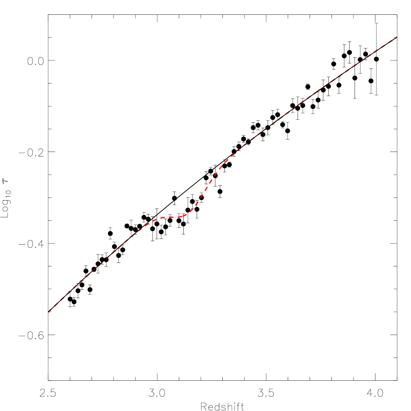
The parameters which minimize $\chi^{2}$ for our standard definition of the wavelength range spanned by the forest ($1080-1160$ Å) are given in Table 1. (Two technical comments are necessary. First, only the longest wavelength range has sufficient wavelength coverage to constrain well all three Gaussians which make up the continuum. Therefore, in practice, the parameters which define the continuum were set using the largest wavelength range, $1060-1180$ Å, and were held fixed when analyzing the standard and the shorter ranges. Second, as we show in Appendix B.2 below, there is a calibration problem at the very blue end of the spectrograph. This affects the pixels corresponding to the redshifts $z_{\alpha}<2.5$ in the forest, so the minimization procedure was run using only pixels with $z_{\alpha}\geq 2.6$.) Two sets of values are shown: the first is for the entire sample, and the second is for a subset which has a higher signal-to-noise ratio (see Section 4.2). The quoted errors are from bootstrap resampling, with replacement, of entire QSO spectra. The slope of the continuum, $c_{1}=-1.56$ is the same as that reported by Vanden Berk et al. (2001) in their analysis of SDSS QSOs. The exact shape is shown by dotted lines in Figure 15. The smooth evolution of the optical depth, $t_{0}=0.0028$ and $t_{1}=3.69$, is in reasonable agreement with previous analyses of low resolution spectra (e.g. Press, Rybicki & Schneider 1993). The fact that $t_{2}=-0.060$ is less than zero suggests that $\tau_{\rm eff}$ decreases by about 10 percent at $z_{\alpha}=t_{3}-1=3.15$. Figure 4 shows this feature superimposed on the otherwise smooth evolution of the effective optical depth.

The procedure above requires minimization of a function which depends nonlinearly on the parameters to be fitted. Press, Rybicki & Schneider (1993) discuss how and why one might approximate a nonlinear function of the sort above by one which depends linearly on the parameters to be fitted. Since we have a good idea of where the features in the continuum and in the mean transmission might be (from the composite spectra), we could experiment with performing simpler linear fits of the sort they discuss, although we have not done so here. A modification to the method, which we have also not explored, is to weigh each pixel by the inverse of the noise when defining $\chi^{2}$.

This method is very different from any in the literature. In Appendix A, we describe a technique which is more closely related to that introduced by Oke & Korycansky (1982), and developed further by Schneider, Schmidt & Gunn (1991) and Press, Rybicki & Schneider (1993). The next subsection shows that both techniques give consistent results.

Figure 4: The effective optical depth as a function of redshift $z_{\alpha}=\lambda_{obs}/\lambda_{\alpha}-1$: the average is over all pixels which have the same $z_{\alpha}$ and which have restframe wavelengths which lie in the Ly$\alpha$ forest region between $1080-1160$ Å. Dashed line shows the mean evolution obtained from the $\chi^{2}$ procedure described in Section 3.1. Filled circles show the estimate from the iterative technique described in Appendix A. Solid line shows a simple power-law: $\tau_{\rm eff}\propto(1+z_{\alpha})^{3.69}$.

3.2 Result: The evolution of the effective optical depth

Having determined how the mean continuum depends on restframe wavelength, and how the mean transmission depends on redshift $z_{\alpha}$, we can now estimate how the effective optical depth $\tau_{\rm eff}\equiv-\ln\bar{F}$ evolves (note that we used $T$ for $\bar{F}$ in the previous subsections). The dashed line in Figure 4 shows the effective optical depth obtained from the $\chi^{2}$ technique described in the previous section (i.e., from the parameter values in Table 1). To highlight the feature at $z\sim 3.2$, the solid line shows the smoother function $\tau_{\rm eff}\propto(1+z_{\alpha})^{3.69}$.

The solid circles in Figure 4 show $\tau_{\rm eff}$ as a function of $z_{\alpha}$, estimated using the iterative technique described in Appendix A. The different circles show averages over all pixels which have the same observed wavelength $\lambda_{obs}=\lambda_{\alpha}(1+z_{\alpha})$, and which have restframe wavelengths which lie in the Ly$\alpha$ forest region between $1080-1160$ Å. The error bars were computed by bootstrap re-sampling, with replacement, the entire sample 50 times (entire QSO spectra, rather than individual pixels, are re-sampled). The error bars show the standard deviation of the 50 mean values. The bootstrap procedure also allows an estimate of bin-to-bin correlations: each of the circles in Figure 4 is correlated with its first nearest neighbour on either side, but the covariances fall rapidly for more distant pairs.

Figure 4 shows that our estimates of the evolution of the effective optical depth are in good agreement with each other (compare dashed line with solid circles). Although $\tau_{\rm eff}(z_{\alpha})$ increases with increasing redshift, there is a statistically significant change in the evolution around $z_{\alpha}\approx 2.9-3.2$. Flux calibration problems are not the origin of this feature (see Appendix B.2). Although our two techiniques might produce small systematic errors in the determination of the mean transmission, these errors are not expected to produce such a relatively sudden change as a function of redshift.

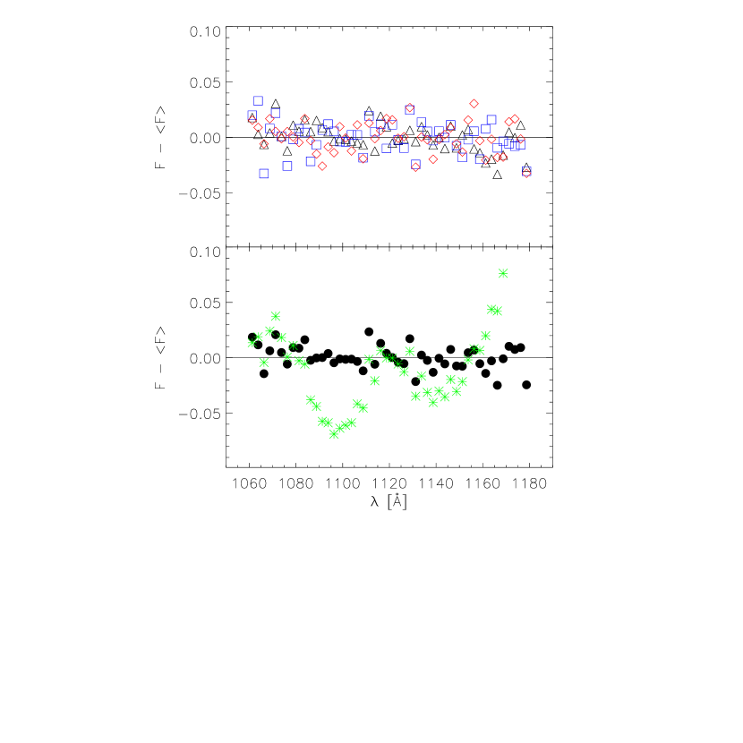
To test if our estimate of the continuum shape is reasonable, we computed the residual of each pixel at $z_{\alpha}$ from the mean transmission at $z_{\alpha}$. If we have estimated the continuum (and hence the mean transmission $T$) correctly, then a plot of the residuals $f_{i}/C-T$ versus $\lambda_{rest}$ (rather than $\lambda_{obs}$, which is effectively what the x-axis in Figure 4 is) should not show any trend. (Recall that $\langle f_{i}/C-T\rangle=\langle f_{i}/(C+c_{i})+f_{i}/(C+c_{i})(c_{i}/C)\rangle-T=\langle t_{i}\rangle-T+\langle f_{i}/(C+c_{i})(c_{i}/C)\rangle=\langle f_{i}/(C+c_{i})\rangle\langle c_{i}/C\rangle=0$, and that the $\chi^{2}$ method is constructed to satisfy this condition.) Triangles, squares and diamonds in the top panel in Figure 5 show the mean value of the measurement averaged over the pixels from QSOs at low ($z<3.2$), medium ($3.2<z<3.7$) and high redshift ($z>3.7$). The absence of any trends suggests that our estimate of the continuum is, indeed, accurate. Just for comparison, the stars in the bottom panel show the mean of the residuals computed using the featureless $\alpha_{\lambda}=-1.56$ power-law continuum. Note the structures which coincide with the positions of the emission lines discussed previously.

Figure 5: Difference from the mean transmission at a given redshift $z_{\alpha}$, plotted as a function of restframe wavelength rather than redshift. Triangles, squares and diamonds in the top panel show measurements averaged over QSOs at low ($z<3.2$), medium ($3.2<z<3.7$) and high ($z>3.7$) redshifts. Top panel shows no trends, suggesting that our estimate of the continuum is reasonable. Filled circles in bottom panel show the average over all redshift bins, and stars show the same test but using the featureless $\alpha_{\lambda}=-1.56$ power-law continuum. In this last case there is significant structure, illustrating that neglecting the emission features is a bad approximation.

In summary: we have described two methods which allow one to solve simultaneously for the shape of the QSO continuum in the restframe wavelength range between the Ly$\alpha$ and Ly$\beta$ emission lines and the evolution of the mean transmission in the Ly$\alpha$ forest. The two methods lead to the same conclusion—the inferred continuum is not a featureless power-law but has bumps in it; these are almost certainly emission lines from the QSO. It is important to account for these features in the continuum when estimating the mean transmission in the Ly$\alpha$ forest. Although the effective optical depth increases with increasing redshift, it does not evolve smoothly: there appears to be little or no evolution around $z_{\alpha}\sim 3$. The next section studies the evidence for this feature in more detail.

4 Tests of systematic effects on the estimated evolution

This section discusses a number of possible systematic effects which might have given rise to a feature in the mean transmission, but argues that none of these are the cause.

4.1 The QSO selection algorithm

The $\chi^{2}$ method solves simultaneously for the mean transmission and the mean continuum. The technique works best when the sample covers a large range in redshift. Figure 6 shows the number of pixels in our sample at each redshift $z_{\alpha}$, when the forest is defined by our standard wavelength interval 1080–1160 Å (the middle of the three intervals shown in Figure 3). Each spectrum contains about 120 pixels which fall in the Ly$\alpha$ forest, and we have on the order of $10^{3}$ spectra. Therefore, we have a large number of pixels from which to determine the shape of the continuum and the transmission, and the figure shows that they do indeed span a large redshift range.

Figure 6: Distribution of Ly$\alpha$ forest redshifts $z_{\alpha}$ in our sample. Each pixel at observed wavelength $\lambda_{obs}$, which has a restframe wavelength in the Ly$\alpha$ forest region defined in the main text, is assigned a redshift $z_{\alpha}=\lambda_{obs}/\lambda_{\alpha}-1$. There are typically of order 120 pixels per spectrum which lie in the Ly$\alpha$ forest; with $\sim 1000$ spectra, this means there are about 120,000 Ly$\alpha$ forest pixels in total. The drop in numbers around $z\sim 3.2$ is a consequence of the SDSS QSO selection procedure, as discussed in Appendix B. The gaps at $z\sim 3.59$ and $z\sim 3.84$ correspond to the O I (5577 Å) sky-line and interstellar Na I (5894.6 Å), respectively; the observed wavelength range $5570\leq\lambda\leq 5590$ Å was removed from our analysis, as were the pixels affected by the Na I line.

However, two features in Figure 6 deserve further comment. First, there are obvious drops at $z\sim 3.59$ and at $z\sim 3.84$. The SDSS pipeline reductions do not completely subtract the sky-line O I ($5577$ Å). This wavelength range corresponds to a Ly$\alpha$ redshift of $z\sim 3.59$; hence the gap in the Figure. Therefore, we removed from our analysis the observed wavelength range $5570\leq\lambda\leq 5590$ Å. The gap at $z\sim 3.84$ is due to interstellar Na I; the pixels affected by this line (at 5894.6 Å) were also removed from our analysis. Second, there is a more gradual and extended dip in counts around $z\sim 2.8-3.4$. The Ly$\alpha$ emission line passes from the $g^{*}$ to the $r^{*}$ band at $z\sim 3.5$. Therefore, the observed colors of QSOs change relatively rapidly in this regime, and so one might worry that the color–based algorithm which SDSS uses for targetting QSO candidates for observation is less accurate at these redshifts. In particular, one might worry that the dip in counts evident in Figure 6 signals the fact that the selection algorithm chooses a biased subset of the complete population at these redshifts. This is of particular concern because the feature in $\tau_{\rm eff}(z)$ occurs in this redshift range.

A detailed discussion of the effect of the color–based selection is presented in Appendix B, which argues that the selection does not result in a biased measurement of the mean transmission. It also argues that, if there are inaccuracies in how the SDSS spectrograph is calibrated, they do not give rise to a feature in the evolution of the mean transmission.

4.2 The ratio of signal-to-noise

Figure 7: Distribution of signal-to-noise ratios in our sample redward (left) and blueward (right) of the Ly$\alpha$ emission line. Solid and dashed histograms in the panel on the right are for spectra with $S/N$ ratios (computed redward of the Ly$\alpha$ emission line) which are greater than and less than 4.

Figure 8: Signal-to-noise ratios in the Ly$\alpha$ forest as a function of redshift. Top and bottom panels show results for spectra with larger/poorer ratios redward of $\lambda_{\alpha}$.

Figure 9: Evolution of the effective optical depth estimated using spectra which have low (stars) and high (circles) signal-to-noise ratios redward of the Ly$\alpha$ emission line. Dashed line (same as in Figure 4) shows the evolution inferred for the entire sample. The feature in $\tau_{\rm eff}$ is more obvious in the spectra which have larger signal-to-noise ratios.

The signal-to-noise ratio in our sample is low. We would like to be sure that the evolution of $\tau_{\rm eff}$ does not depend on $S/N$. The panel on the left of Figure 7 shows the distribution of the typical $S/N$ when the ratio is computed on the red side of $\lambda_{\alpha}$ in each spectrum. The panel on the right shows the distribution of typical $S/N$ ratios in the Ly$\alpha$ forest region of each spectrum for QSOs with large (solid) and small (dashed) $S/N$ ratios redward of $\lambda_{\alpha}$.

Figure 8 shows the distribution of $S/N$ ratios in the forest as a function of redshift. The two panels are for spectra with $S/N>4$ and $S/N<4$ redward of the Ly$\alpha$ emission line. The upper panel shows that the higher redshift spectra tend to have lower $S/N$ ratios. Comparison with the typical noise curves in different panels of Figure 14 suggests that the noise in the Ly$\alpha$ forest is approximately the same at all redshifts. If the noise does not change with redshift, then the fact that the mean transmission is smaller at high redshift means that the typical $S/N$ ratios will also be smaller at high redshift. This is qualitatively consistent with the trend in Figure 8. Therefore, Figure 8 suggests that if we keep only spectra with larger values of $S/N$ (i.e., we use only those spectra which contribute to the top panel), then we will not introduce any severe redshift dependent cuts into the sample. An estimate of $\tau_{\rm eff}(z)$ in the higher signal-to-noise sample should therefore be fair. Note that it is important to make this cut using the $S/N$ ratio redward of Ly$\alpha$; if the noise is approximately the same for all spectra, then eliminating spectra with small $S/N$ ratios in the Ly$\alpha$ forest region biases the sample towards larger transmission.

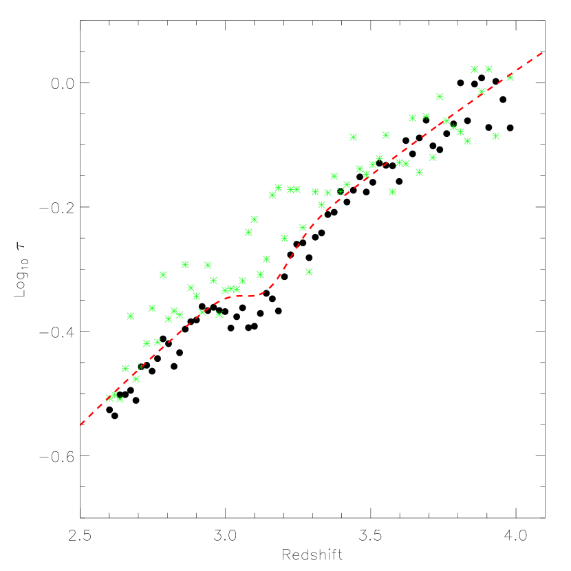
Figure 9 shows the evolution of the effective optical depth estimated using spectra which have low (stars) and high (circles) signal-to-noise ratios redward of the Ly$\alpha$ emission line. Dashed line (same as in Figure 4) shows the evolution inferred for the entire sample. There are many fewer low $S/N$ spectra, so the stars scatter wildly. In contrast, the feature in $\tau_{\rm eff}$ is more obvious in the spectra which have S/N$>4$ (796 of the 1061 spectra in our full sample form this higher S/N subsample). The plots which follow show results from the higher $S/N$ subsample only.

4.3 Dependence on smoothing scale

The $\chi^{2}$ estimate of $\tau_{\rm eff}$ comes from a sum over the fluxes in each pixel, so it can be thought of as an estimate which smoothes the data as little as possible. It is interesting to see if the inferred evolution depends on how the measurement is smoothed. For example, we could have chosen to compute the mean transmission averaged over the spectrum of each QSO: i.e., we could average the transmission over all the Ly$\alpha$ forest pixels in the spectrum of each object, and plot it as a function of the mean redshift of the forest (recall that this redshift depends on the redshift of the QSO). Or we could split the Ly$\alpha$ forest of each spectrum into two pieces, or four pieces, or eight, etc., down to the minimum possible scale which is set by the SDSS pixel size, and plot the mean transmission as a function of the mean redshift in the half-spectrum, the quarter-spectrum, etc. There is no compelling reason for prefering one choice to another since, whatever sets the physical scale in the forest (e.g., the Jeans smoothing scale is expected to be about 30 km s^-1), the SDSS spectrograph does not resolve it.

Figure 10: Evolution of the effective optical depth in the Ly$\alpha$ forest: dependence on smoothing scale. Solid curve shows the evolution derived from applying the $\chi^{2}$ technique on the $S/N>4$ sample; dashed curves show the same, except that they have been offset from the solid curve for clarity. Symbols, which have also been offset for clarity, show the mean $\tau_{\rm eff}$ derived from cutting the spectra in half (top), in quarters (second from top), in eight (third from top), and so on, down to 64 pieces, and plotting versus the median redshift $z_{\alpha}$ in the half-spectrum, the quarter-spectrum, etc. Evidence for a feature in $\tau_{\rm eff}$ becomes apparent only when the size over which the measurement is averaged is smaller than the size of the feature.

Figure 11: Dependence of the effective optical depth on the definition of the Ly$\alpha$ forest. Different sets of curves and symbols show results for three definitions of the wavelength range spanned by the Ly$\alpha$ forest: $1060-1180$ Å (bottom), $1080-1160$ Å (middle), and $1100-1150$ Å (top). The upper and lower sets have been shifted upwards and downwards by 0.2 in $\log_{10}\tau$. Smooth line shows the evolution of $\tau_{\rm eff}$ determined by the $\chi^{2}$ technique applied to the $S/N>4$ sample (see Table 1); dashed and dotted curves show the same, except that they have been offset upwards and downwards by 0.2 in $\log_{10}\tau$. Triangles, squares and diamonds show measurements from QSOs at low ($z<3.2$), medium ($3.2<z<3.7$) and high ($z>3.7$) redshifts. Error bars were computed by bootstrap re-sampling as described in the text.

Figure 12: Evolution of the effective optical depth in the Ly$\alpha$ forest: dependence on continuum shape and normalization. Filled circles show our standard, crosses result from assuming a featureless power-law, diamonds from retaining features, but normalizing by the region in front of Si IV instead of C IV, and stars use both regions to normalize the spectra. The feature in $\tau_{\rm eff}$ is present in all cases.

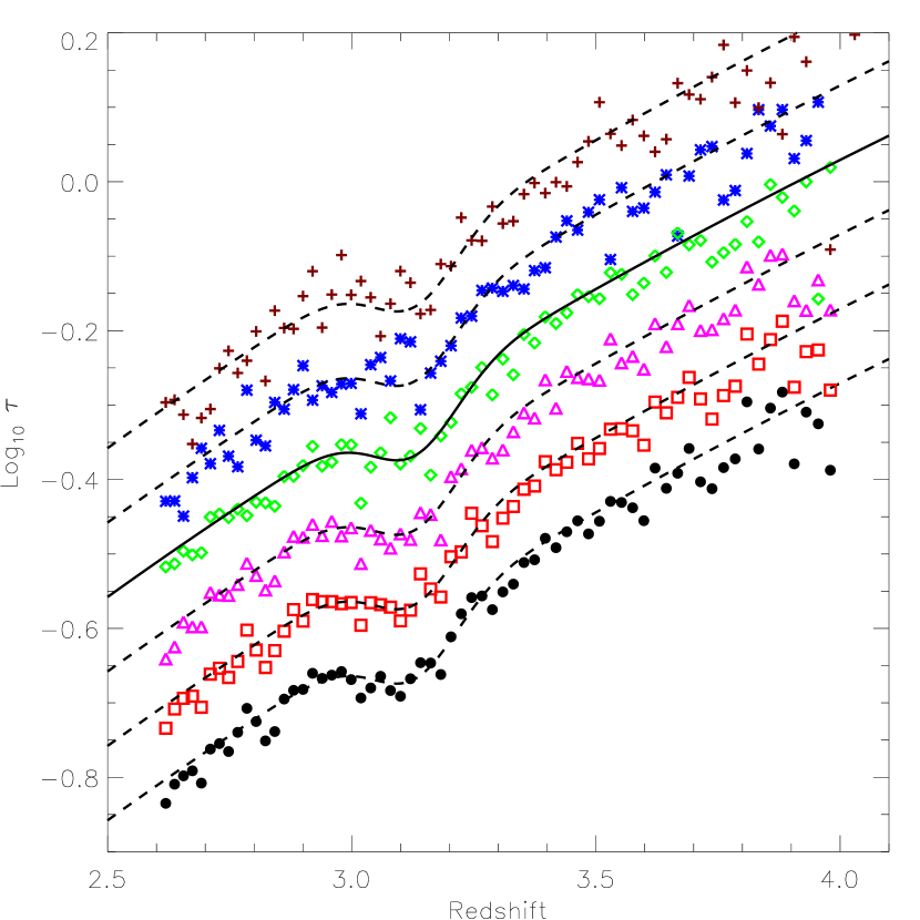
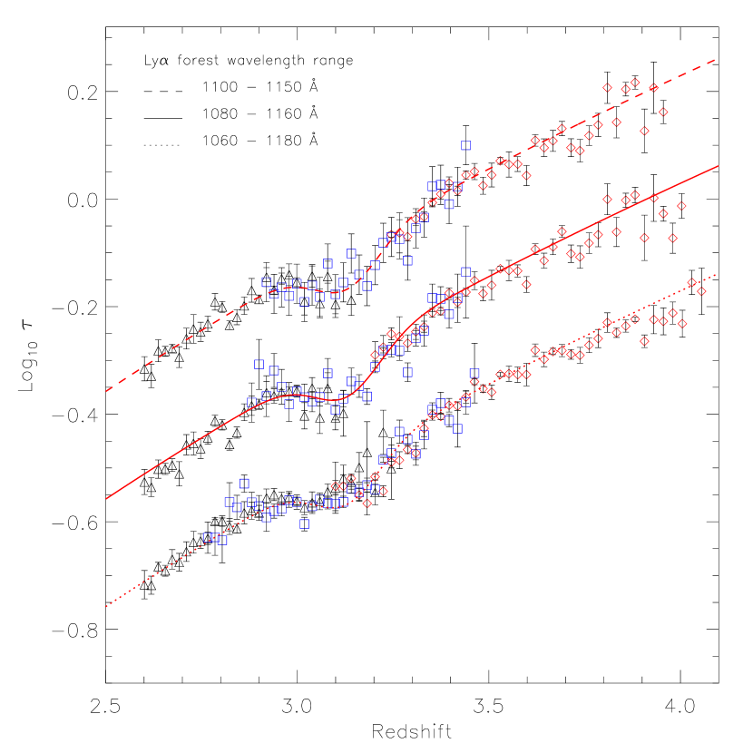
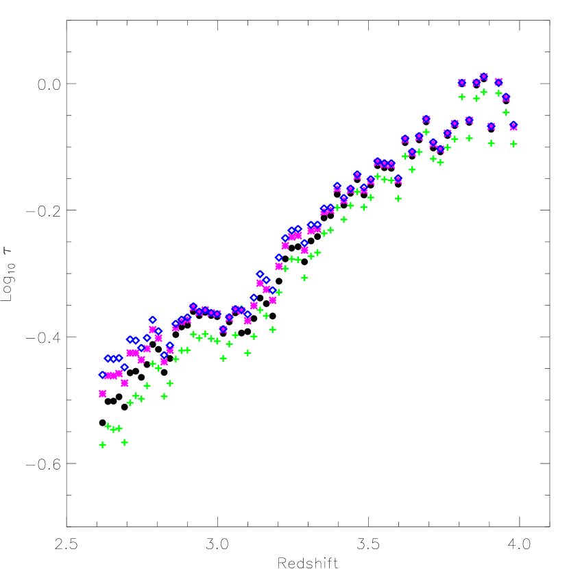
Figure 10 shows the evolution of the effective optical depth in the Ly$\alpha$ forest as a function of smoothing scale. The solid curve shows the evolution derived from applying the $\chi^{2}$ technique to the sample with higher $S/N$ (parameters are in Table 1); dashed curves show the same, but have been offset from the solid curve for clarity. Symbols, which have also been offset for clarity, show the mean $\tau_{\rm eff}$ derived after cutting the spectra in half (top), in quarters (second from top), in eight (third from top), and so on, and plotting versus the median redshift $z_{\alpha}$ in the half-spectrum, the quarter-spectrum, etc. The figure shows that evidence for a feature in $\tau_{\rm eff}$ becomes apparent only when the size over which the measurement is averaged is smaller than the size of the feature. Once the smoothing scale is smaller than $\Delta\lambda_{obs}\approx 40\AA$, i.e., about 3,000 km s^-1, the feature in $\tau_{\rm eff}$ is robust.

Although the evolution of $\tau_{\rm eff}$ inferred from mean value statistics does not depend on the bin size, the estimated evolution from median value statistics does. This is a signature that the underlying distribution of flux decrements is non-Gaussian. [A non-Gaussian distribution is not unexpected; it is seen in hydro-dynamical simulations of the Ly$\alpha$ forest, and there are theoretical models relating it to the non-Gaussian distribution of mildly nonlinear density fluctuations (e.g., Gaztañaga & Croft 1999).] Appendix C summarizes the effects of using median rather than mean value statistics to make all our estimates. It shows that, for the median as for the mean, a feature in $\tau_{\rm eff}(z)$ appears at $z\sim 3.2$.

4.4 Dependence on definition of forest

Figure 11 shows that the feature in $\tau_{\rm eff}$ is not caused by QSOs in one particular redshift range, nor does it depend on the precise wavelength range used to define the forest. The different sets of curves show results for three different choices of the wavelength range spanned by the Ly$\alpha$ forest: the middle curve and associated symbols show results for the wavelength range $1080-1160$ Å; the upper and lower curves, which have been shifted by $\log_{10}\tau=\pm 0.2$ for clarity, show results for the wavelength ranges $1100-1150$ Å and $1060-1180$ Å, respectively. Results for the larger range are more likely to be affected by inaccuracies in our continuum fit which arise from the fact that the Ly$\alpha$ emission line at $\lambda_{\alpha}=1215.67$ Å has a tail which extends to shorter wavelengths (cf. Figures 3 and 5). The shortest wavelength range is more conservative about the accuracy of the continuum fit in the vicinity of the emission line.

In each set of curves, triangles, squares and diamonds show $\log_{10}\tau_{\rm eff}$ estimated from the mean transmission in the pixels of spectra of QSOs in the redshift ranges $z<3.2$, $3.2<z<3.7$, and $z>3.7$. The figure shows that the measurements from the three redshift ranges fit smoothly onto each other and overlap (the amount of overlap depends, of course, on the wavelength range the Ly$\alpha$ forest spans), even though the SDSS sample in the middle redshift range is incomplete (Appendix B). Also, note that the feature in $\tau_{\rm eff}$ does not depend on the wavelength range used to define the Ly$\alpha$ forest—although the dip is perhaps more obvious in our most conservative definition of the forest (top curve) than when the forest overlaps the tails of Ly$\alpha$ emission line (bottom).

4.5 Dependence on the shape and normalization of the continuum

One of the novel features of the continuum we use is the incorporation of non-power-law features (such as the bumps at $\sim 1070$ Å and $\sim 1120$ Å). Other studies of $\tau_{\rm eff}$ using similarly low resolution spectra (e.g. Schneider, Schmidt & Gunn et al. 1991) do not incorporate these features. To compare our results with theirs, we repeated the analysis assuming that the continuum was a featureless power-law with slope $\alpha_{\lambda}=-1.56$ (see, e.g., the smooth solid lines in Figure 1).

Filled circles in Figure 12 show $\tau_{\rm eff}(z)$ for our standard definition of the continuum, and crosses show the result of using the featureless power-law. Since the power-law continuum has less flux than our standard, the inferred mean transmission is always higher, so the associated $\tau_{\rm eff}$ always slightly lower. Retaining features in the continuum, but normalizing by the flux in the range $1350-1370$ Å (the region just blueward of the Si IV emission line) instead of $1450-1470$ Å (diamonds in Figure 12), or normalizing by the flux in both regions (stars in Figure 12), makes little difference at high redshifts, but begins to matter at lower redshifts. A glance at the composite spectra in Figure 14 shows why: a power-law which is normalized to fit the range $1450-1470$ Å only provides a good fit to the region in front of Si IV at higher redshifts, but systematically underestimates the flux there by a small amount at lower redshifts. Changing the normalization increases the flux in the continuum, which reduces the inferred transmission and increases the effective optical depth. Although the evolution of $\tau_{\rm eff}$, particularly at lower redshifts does depend on how we normalize the spectra, the feature in $\tau_{\rm eff}$ is present, at the same redshift, in all cases.

We have also examined (and excluded) the possibility that the feature is produced by intrinsic absorption in a subset of QSO in our sample by 1) determining that the optical depth is not a function of velocity of the absorber from the emission redshift, and 2) determining that the effect is not influenced by the well-known velocity shift of C IV emission (e.g. Richards et al. 2002b).

5 Discussion

When applied to a sample of 1061 QSO spectra drawn from the SDSS database, two methods—which solve simultaneously for the shape of the QSO continuum and for the evolution of the mean transmission—give consistent results. Both methods show that the continuum in the wavelength range between the Ly$\alpha$ and Ly$\beta$ emission lines is not smooth, but has features in it. The two methods also show that although the effective Ly$\alpha$ optical depth decreases smoothly with time, $\tau_{\rm eff}\propto(1+z)^{3.8\pm 0.2}$, it drops by about 10 percent from $z\sim 3.3$ to $z\sim 3.1$, and it recovers to the original smooth scaling by $z\sim 2.9$.

Figure 13: Comparison of measurements of the evolution of the effective optical depth in the Ly$\alpha$ forest. Stars, diamonds, squares and small filled circles show measurements from 42 low resolution spectra by Sargent, Steidel & Bocksenberg (1989), 33 from Schneider, Schmidt & Gunn (1991), 42 from Zuo & Lu (1993), and the subset of 796 QSOs in the SDSS sample which had $S/N>4$ and were studied in this paper. Triangles and large filled circles show measurements in $\sim 10$ higher resolution spectra by McDonald et al. (2000) and Schaye et al. (2000). Dotted line shows the evolution reported by Press, Rybicki & Schneider (1993), and dashed line shows the evolution given in Table 1.

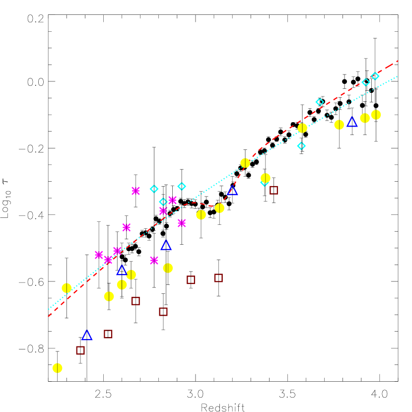
A comparison of our measurement of $\tau_{\rm eff}$ with the findings of other authors is shown in Figure 13. Stars, diamonds, squares and small filled circles show measurements from low resolution spectra of 42 QSOs by Sargent, Steidel & Bocksenberg (1989), 33 QSOs from Schneider, Schmidt & Gunn (1991), 42 QSOs from Zuo & Lu (1993), and 796 QSOs from the SDSS sample studied in this paper (the 796 spectra with $S/N>4$ out of the full sample of 1061 QSOs; the Ly$\alpha$ forest was defined to span the range $1080-1160$ Å). Dotted line shows the evolution in the Schneider, Schmidt & Gunn sample reported by Press, Rybicki & Schneider (1993), and dashed line shows the evolution given in Table 1. Large filled circles and open triangles show measurements from high resolution high signal-to-noise spectra by Schaye et al. (2000) and McDonald et al. (2000)—but note that although the two sets of analyses differed (McDonald et al. quote results in coarser redshift bins than do Schaye et al.), they were performed on essentially the same set of $\sim 10$ QSO spectra.

Figure 13 shows that our measurements are in general agreement with previous work based on low resolution, low signal-to-noise spectra (compare small filled circles with stars and diamonds). However, because our sample is so much larger than any previously available, it is possible to measure the evolution of $\tau_{\rm eff}$ in smaller redshift bins than was possible previously. The figure also shows that our measurement of $\tau_{\rm eff}$ results in about ten percent less transmitted flux than suggested by recent measurements from higher resolution spectra (triangles and large circles). At higher redshifts, where the absorption is large, it becomes increasingly difficult to estimate the continuum reliably for high resolution spectra. This, together with small number statistics may account for some of the discrepancy at $z>3.5$. At lower redshifts, some of the discrepancy may arise because damped Ly$\alpha$ systems and/or metal lines, which become increasingly abundant at low redshifts, have been removed from the higher resolution spectra, but are still present and contributing to the effective optical depth in our sample. Although the mean transmission measured in noisy and low resolution spectra may yield a biased measure of the slope and amplitude of the evolution of the true effective optical depth (e.g., Steidel & Sargent 1987), it is difficult to see why this bias should lead to a feature in $\tau_{\rm eff}(z)$. Thus, whereas the slope and amplitude of the evolution we find should be calibrated against simulations and other measurements, we feel we have strong evidence that the effective optical depth of the IGM changed suddenly around $z\sim 3.2$.

The gradual evolution of the effective optical depth, and the strength of the feature superposed on it, both have implications for how the temperature and the photo-ionization rate evolve (equation 1). It is interesting that the feature we see in $\tau_{\rm eff}$ occurs at the same redshift range as the factor of two increase in temperature that Schaye et al. (2000) detected. Schaye et al. interpreted their measurement as evidence that He II reionized at $z\sim 3.5$. Hydrodynamical simulations show that our measurement of the evolution of $\tau_{\rm eff}$ is consistent with this interpretation (Theuns et al. 2002). The simulations can also help us understand if the mean scaling $\tau_{\rm eff}\propto(1+z)^{3.8\pm 0.2}$ we see leads to reasonable values for the amplitude and evolution of $\Gamma$. It would be a significant accomplishment if the simulations were also able to reproduce the evolution of the skewed distribution around the mean—the latter being quantified by how the median optical depth depends on smoothing scale and on redshift (Figure 23). This is the subject of ongoing work.

The reionization of He II is expected to be proceed more gradually than for H I. The fact that the feature appears relatively gradually in our data can be used to place constraints on how patchy the onset of reionization was. When the SDSS survey is complete, it will be possible to compile a data set which is large enough to study different portions of the sky separately. This will provide an even more direct constraint on the homogeneity of the Universe at the epoch of He II reionization.

Acknowledgments

This project started when Tom Theuns visited Fermilab in September 2001. We would like to thank him for a discussion which led to this measurement, and for helpful correspondence since then. We also thank Paul Hewett, Patrick McDonald, Celine Peroux, and Uros Seljak.

Funding for the creation and distribution of the SDSS Archive has been provided by the Alfred P. Sloan Foundation, the Participating Institutions, the National Aeronautics and Space Administration, the National Science Foundation, the U.S. Department of Energy, the Japanese Monbukagakusho, and the Max Planck Society. The SDSS Web site is http://www.sdss.org/.

The SDSS is managed by the Astrophysical Research Consortium (ARC) for the Participating Institutions. The Participating Institutions are The University of Chicago, Fermilab, the Institute for Advanced Study, the Japan Participation Group, The Johns Hopkins University, Los Alamos National Laboratory, the Max-Planck-Institute for Astronomy (MPIA), the Max-Planck-Institute for Astrophysics (MPA), New Mexico State University, the University of Pittsburgh, Princeton University, the United States Naval Observatory, and the University of Washington.

Appendix A An iterative procedure for estimating the mean continuum

We begin by assuming that the continuum is a power-law,

$$f_{cont}(\lambda_{rest})\propto\lambda_{rest}^{\alpha_{\lambda}},$$ (A1)

normalized to have the same flux as that observed in the restframe wavelength range $1450-1470$ Å:

$$\sum_{1450}^{1470}f_{obs}=\sum_{1450}^{1470}f_{cont}.$$

This wavelength range lies in front of the C IV emission line, and is free of obvious emission and absorption lines (e.g., Press, Rybicki & Schneider 1993).

Figure 14: Restframe normalized spectra (i.e. wavelengths were transformed to the restframe of the QSO, and the flux density of each QSO spectrum was normalized in the wavelength region $1450-1470$ Å, as described in the text); different panels show results for different redshift bins. The solid curve in each panel shows the mean value of the flux density in all the normalized restframe spectra in the redshift bin shown. The lower dotted curve shows the observed rms scatter above the mean value, and upper dotted curve shows the 95 percentile value as a function of restframe wavelength. The thin line in the bottom of each panel shows the typical value of the noise for individual spectra. (The noise on each composite spectrum is a factor of $\sim 1/\sqrt{100}$ smaller.) Subtracting the noise in quadrature from the observed rms scatter (i.e., from the lower of the two dotted curves) gives the dashed curve. The curve which rises smoothly from right to left shows a power-law of slope $\alpha_{\lambda}=-1.56$. The bumpy line was obtained by simply shifting the dashed curve in the region shortward of $\lambda_{\alpha}$ upwards or downwards until its local minima touched the extrapolated power-law. The vertical lines on the left of each panel show three different wavelength regions adopted in defining the Ly$\alpha$ forest: 1060–1180 Å (dashed), 1080-1160 Å (dot-dot-dot-dashed), and 1100–1150 Å (dot-dashed).

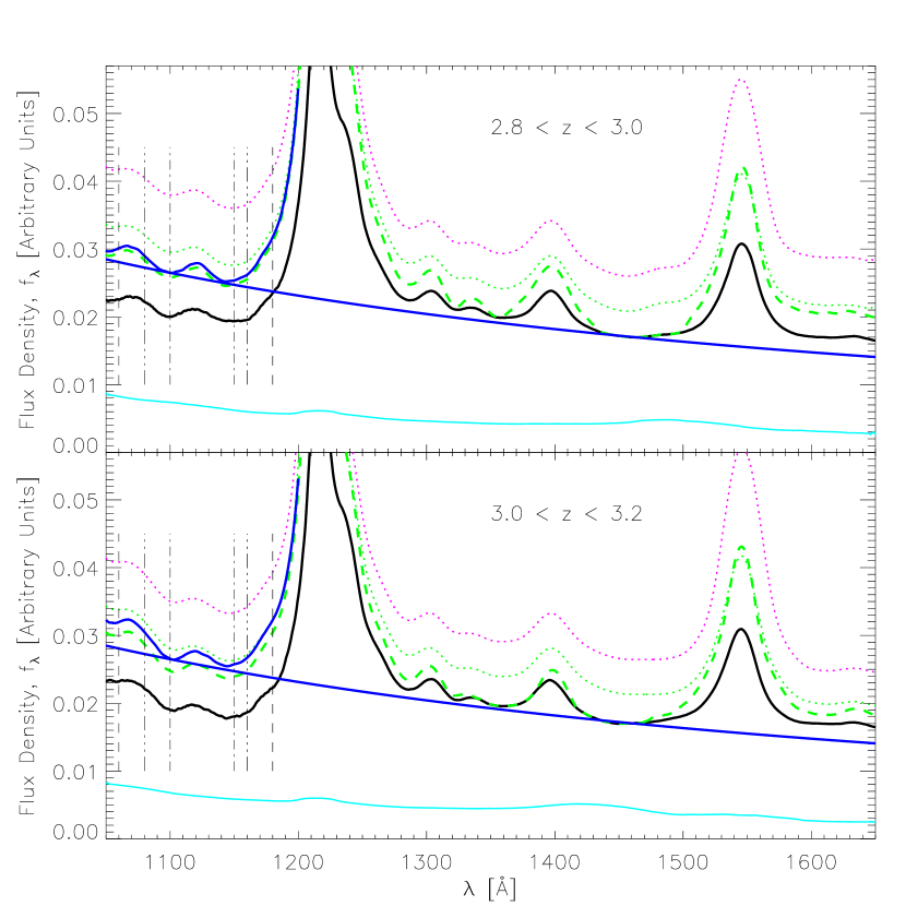
Fig. 14. – Continued.

From a composite spectrum of about 2,400 SDSS QSO spectra which span a range of redshifts, Vanden Berk et al. (2001) estimate that $\alpha_{\lambda}=-1.56$ in the interval $1280-5000$ Å. The smooth lines in Figure 1 show that this power-law continuum shape provides a reasonable description of the individual spectra in our sample. Note that this slope is rather different from the value $\alpha_{\lambda}=-1.07$ used by other authors (see Vanden Berk et al. 2001 for further discussion).

The different panels in Figure 14 show results obtained by averaging over QSOs in the redshift bins indicated in the top right corners. The thick solid line in each panel shows the observed composite spectrum, which we will call $F_{50}$ since it is very close to the median value in each restframe wavelength bin. The $\alpha_{\lambda}=-1.56$ power-law (the same in all panels) provides a reasonable fit redward of the Ly$\alpha$ line, but lies significantly above the composites blueward of $\lambda_{\alpha}$. This difference is larger at higher redshift, qualitatively consistent with the expectation that there is more absorption in the forest at high redshift. The lower dotted curve in each panel shows the rms scatter above the mean composite spectrum, and the upper dotted curve shows the curve traced out by the 95 percentile level. These curves provide estimates of the scatter around the mean spectrum, but almost all of this scatter is due to the noise. The solid curve in the bottom of each panel shows the typical value of the noise: it was obtained by squaring the individual noise estimates for each pixel, computing the average of these squared values at each bin in restframe wavelength, and taking the square root. A comparison of these noise estimates with the observed composites shows that the typical signal-to-noise ratio is $\sim 5$ longward of $\lambda_{\alpha}=1215.67$ Å, and only $\sim 3$ shortward of $\lambda_{\alpha}$. The dashed lines show the result of subtracting the noise in quadrature before computing the rms scatter around the mean curve (i.e., the square root of $\sum_{i}(f_{i}-F_{50})^{2}-n_{i}^{2}$). Except in the vicinity of the emission lines, most of the observed scatter redward of $\lambda_{\alpha}$ is due to the noise. This is consistent with Figure 2 in the main text which showed that the intrinsic scatter around the mean continuum shape is small.

Redward of $\lambda_{\alpha}$, the local minima of the dashed lines track the height of the mean curve, $F_{50}$, reasonably well. If there were no absorption in the forest, one might expect the same to be true blueward of $\lambda_{\alpha}$. Therefore, the next step, and the one which most closely parallels previous work, would be to extrapolate the power-law fit blueward of $\lambda_{\alpha}$, and use it to estimate the transmission. However, as we have already seen, there appear to be emission lines in between the Ly$\alpha$ and Ly$\beta$ emission lines. Using the $\alpha_{\lambda}=-1.56$ power-law fit blueward of $\lambda_{\alpha}$ and ignoring the bumps in the continuum will lead to biases in our estimate of the mean transmission.

Figure 15: Initial step in the iteration process. Smooth solid line shows the power-law which was used as the first guess for the shape of the continuum. Dashed line shows the result of using the power-law continuum to estimate the mean transmission, then using the mean transmission to correct the observed fluxes, and computing a composite using these corrected fluxes. The large differences between the initial solid and final dashed curves indicates that the method has not yet converged. The actual observed composite is the thin solid line at the bottom of each panel. Labels indicate the median redshift of the QSOs in each panel, and the vertical lines show the asssociated Ly$\alpha$ forest redshifts.

Figure 15: Continued. Final step in the iteration process. Thick solid bumpy line shows the input value of the continuum, and dashed line shows the final value. Dotted line shows the continuum shape determined by the $\chi^{2}$ technique described in Section 3.1. All three estimates are in reasonable agreement in all the panels, they are all significantly different from the initial power-law continuum (smooth thick solid line), and they are very different from the actual observed composite spectrum (thin solid line).

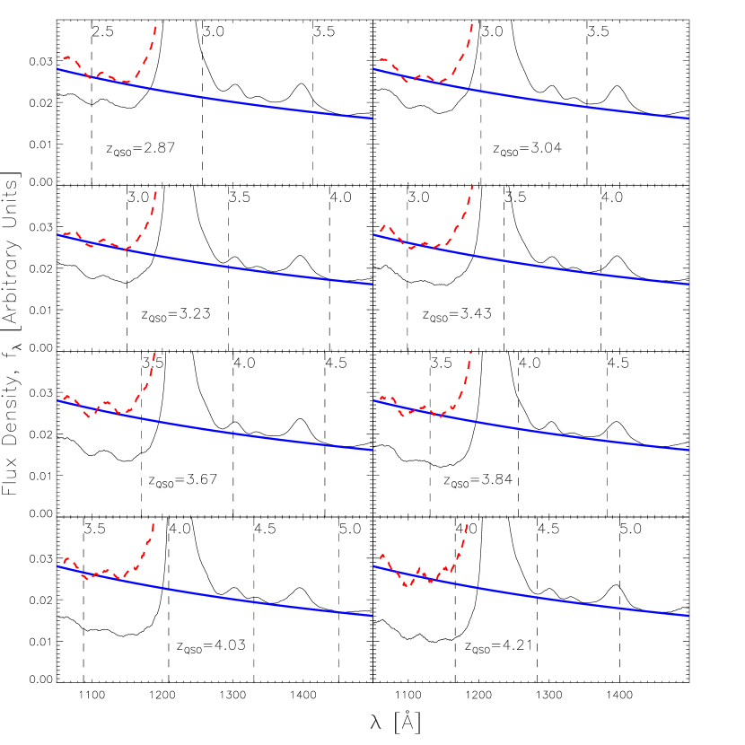
We can correct for this as follows. The extrapolated power-law may have approximately the correct amplitude, but it does not have bumps. On the other hand, the dashed line has bumps in it, but it almost certainly does not have the right amplitude. If the locations of the Ly$\alpha$ forest absorption features in the restframe spectrum of one QSO are uncorrelated with those in most of the others, then if we average many spectra together, the net effect of the forest absorption is to remove flux from the averaged spectrum. If we knew how much was removed, then we could simply add this amount back in to the dashed line. A simple first estimate is to shift the dashed line upwards until it matches the extrapolated continuum. This provides an estimated continuum which has the same amplitude as the power-law fit but has bumps in it. (If we were willing to assume that the continuum does not evolve, then we could simply do this for the lowest redshift bin where the shift is the smallest, and use this shape as the continuum at all other redshifts.) The bumpy solid curves which sit on top of the smooth power-laws in Figure 14 show these estimates of the continuum.

However, these improved estimates of the true continuum are also biased because, in shifting curves upwards by an amount which is independent of $\lambda_{obs}$, we are, in effect, ignoring the evolution of the optical depth over the range in $z_{\alpha}$ spanned by the Ly$\alpha$ forest (recall that this range depends on the redshift bin of the QSOs; Figure 15 shows this dependence explicitly). Since our goal is to measure small changes in the transmission, we must account more carefully for this evolution. Therefore, we have adopted the following iterative procedure.

Our sample of QSOs can be thought of as a collection of pixels. Associated with each pixel $i$ in our sample is a normalized flux density $f_{i}$, an observed frame wavelength $\lambda_{obs,i}$, and a restframe wavelength $\lambda_{rest,i}$. The transmission associated with pixel $i$ is $f_{i}/f_{oldcont}(\lambda_{rest,i})$, where this ratio is computed in the restframe, and $f_{oldcont}(\lambda_{rest})$ denotes our guess for the shape of the continuum. As the initial guess for $f_{oldcont}$, we can use the dashed curves shown in Figure 14, or even the featureless power-law.

The mean transmission $t$ at $z_{\alpha}$ in the Ly$\alpha$ forest is estimated by summing the transmission in those pixels which have the same observed wavelength $\lambda_{obs}=\lambda_{\alpha}(1+z_{\alpha})$ and dividing by the number of such pixels. The estimated mean transmission $t$ is then used to correct the observed flux density in each pixel for the absorption in the forest. That is, we make a new estimate of the continuum associated with each pixel: $f_{newcont,i}=f_{i}/t(\lambda_{obs,i})$, where we have written the transmission as a function of observed wavelength rather than of redshift in the Ly$\alpha$ forest. We then compute a new composite continuum by averaging $f_{newcont,i}$ over all pixels which have the same value of $\lambda_{rest}$, and compare it with the original guess. If the initial guess for the continuum was accurate, then $f_{newcont}\approx f_{oldcont}$ at all $\lambda_{rest}$. If not, we use the new composite as a revised estimate of the continuum (i.e., we set $f_{oldcont}=f_{newcont}$), and iterate until convergence is reached (typically about three or four interations are needed).

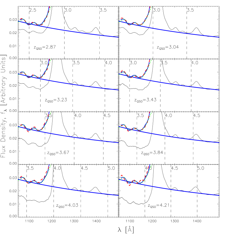
Figure 15 illustrates the process. The different panels show different redshift bins. Vertical dashed lines in each panel show how to translate from restframe wavelength to $z_{\alpha}$. The thin solid line near the bottom of each panel shows the observed composite spectrum. The thick solid line shows the $\alpha_{\lambda}=-1.56$ power-law approximation to the continuum which was used to estimate the mean transmission. The dashed line shows the composite which results from dividing the observed fluxes by the estimated mean transmission and averaging. This new composite is very different from the initial power-law, indicating that the procedure has not converged.

The next set of panels show the result at convergence. The smooth solid line shows the same power-law as before. The bumpy solid line shows the guess for the continuum, and the dashed line shows the composite one gets by correcting all observed fluxes by the mean transmission computed from the bumpy continuum. Notice that the solid and dashed lines are in good agreement with each other. They are also in good agreement with the dotted line which shows the shape of the continuum determined by the $\chi^{2}-$technique described in the main text. All three curves are significantly different from the featureless power-law.

Having determined the mean continuum $f_{cont}$ using this iterative technique, it is possible to measure the mean transmission $\bar{F}\equiv\langle f_{obs}/f_{cont}\rangle$ and therefore $\tau_{\rm eff}\equiv-\ln\bar{F}$ (see Figure 4).

Appendix B Systematic effects

This appendix studies two systematic effects which might give rise to the feature we see in the evolution of the effective depth, and argues that they do not.

B.1 Effect of the SDSS QSO selection algorithm

Figure 16 shows the observed distribution of QSO redshifts in our sample. There is an obvious drop in numbers around $z\sim 3.5$, which, as we describe below, is a consequence of how the colors of quasars change as a function of the SDSS bandpasses. Since the feature we see in $\tau_{\rm eff}(z)$ occurs at slightly lower redshifts (see Figure 4), at least some of the signal comes from the Ly$\alpha$ forests in the spectra of these $z\sim 3.5$ QSOs. This Appendix studies if the feature we see in the optical depth is caused entirely by the QSO selection algorithm. Our approach is to simulate a sample of QSO spectra in which there is no feature in $\tau_{\rm eff}(z)$, select the subset of objects which SDSS would have identified as QSOs, and measure $\tau_{\rm eff}(z)$ in the subset. We then check if the SDSS–selected subset shows any feature in $\tau_{\rm eff}(z)$.

Figure 16: Distribution of QSO redshifts in the SDSS sample. Notice the drop in numbers at $z\sim 3.5$. For QSOs at these redshifts, the Ly$\alpha$ emission line passes from the $g^{*}$ to the $r^{*}$ filter.

The algorithm used by the SDSS collaboration to target QSO candidate objects is described by Richards et al. (2002a). In essence, it uses a stellar locus outlier rejection algorithm, further supplemented with a combination of cuts in the $u^{*}g^{*}r^{*}$, $g^{*}r^{*}i^{*}$, and $r^{*}i^{*}z^{*}$ color-spaces. To test the effects of this selection procedure, we must generate a set of mock QSOs for which redshifts, spectra and colors are known. To generate such a sample using the observed one (which is almost certainly incomplete in the range $3.2<z<3.7$) we must make some assumptions which we describe below.

To generate redshifts of what we will call the complete sample, we draw a straight line in Figure 16 from the observed number at $z=3.2$, $N_{\rm obs}(z=3.2)$, to the observed number, $N_{\rm obs}(z=3.7)$, at $z=3.7$. We then assume that the $N(z)$ distribution of a complete sample would follow $N_{\rm obs}(z)$ over the ranges $z<3.2$ and $z>3.7$, and would follow the smooth straight line we drew for the redshifts in between. Note that this means we are assuming that the observed sample is complete at redshifts $z>3.7$, and also at $z<3.2$. We then generate a distribution of redshifts which follows this model for the complete $N(z)$ distribution.

The SDSS QSO selection is based on color, so our next step is to assign colors to our mock QSOs which are consistent with their redshifts. We do this as follows. Let $z_{\rm sim}$ denote the redshift of a mock QSO. We randomly choose one of the observed QSOs with $z_{\rm obs}>3.7$; we will use it to generate a mock QSO spectrum. The requirement that $z_{\rm obs}>3.7$ insures that none of the QSOs we use to generate our complete sample is from the regime in which we are most worried that the observed sample is incomplete. We then blue- or redshift the observed spectrum to the desired redshift $z_{\rm sim}$.

Figure 17: Comparison of spec-magnitudes obtained by convolving the observed spectra with the SDSS filter response curves, and psf–magnitudes output by the photometric pipeline.

To be specific, suppose that $z_{\rm obs}>z_{\rm sim}$. We are interested in $D_{A}\equiv 1-\langle F\rangle$, the ratio of the flux blueward of Ly$\alpha$ to that of the continuum at the same wavelength. We know that this ratio evolves with redshift (see Figure 4). We would like to generate a sample of spectra in which $\tau_{\rm eff}$ evolves smoothly with $z$, and so we require that $\tau_{\rm eff}$ evolve like a smooth line, e.g. $\tau_{\rm eff}\propto(1+z_{\alpha})^{3.3}$. Let $D_{A}^{\rm fit}(z)$ denote the value of this ratio which gives rise to this smooth evolution in $\tau_{\rm eff}$. Since $\tau_{\rm eff}$ decreases with $z$, the higher-redshift QSO which we have blueshifted to $z_{\rm sim}$ has too little flux in its forest (too much absorption) compared to what we want.

We remedy this as follows. Let $\lambda_{\rm obs}$ denote the observed wavelength of a pixel. It has a Ly$\alpha$ redshift $z_{\rm obs}^{\rm pix}=(\lambda_{\rm obs}/1215.67)-1$. The associated value of the flux decrement is $D_{A}(z_{\rm obs}^{\rm pix})$, and this may be different from $D_{A}^{\rm fit}(z_{\rm obs}^{\rm pix})$. Upon blueshifting, the Ly$\alpha$ redshift we should associate with the pixel is

$$z_{\rm sim}^{\rm pix}=(\lambda_{\rm sim}/1215.67)-1,\qquad{\rm where}\qquad\lambda_{\rm sim}=\lambda_{\rm obs}\,(1+z_{\rm sim})/(1+z_{\rm obs}).$$

Therefore, after fitting the continuum to the blueshifted spectrum, we add $[D_{A}^{\rm fit}(z_{\rm sim}^{\rm pix})-D_{A}^{\rm fit}(z_{\rm obs}^{\rm pix})]\,f_{\rm cont}$ to the flux in each pixel which lies blueward of the Ly$\alpha$ emission line. This ensures that the mean value of $D_{A}(z)$ is consistent with the smooth featureless evolution, but keeps approximately the same statistical fluctuations around the mean that were present at $z_{\rm obs}$. Thus, we have a spectrum in which $f_{\rm sim}/f_{\rm cont}$, in the mean, follows $D_{A}^{\rm fit}(z)$. (In practice, we also add Gaussian noise with rms $\sim 0.05$ chosen to be slightly smaller than that observed.)

Figure 18: Observed and simulated QSO colors as a function of redshift. Dashed lines show the color cuts used by the SDSS collaboration to identify QSO candidates; QSOs on the other side of the lines can also be selected if they meet the stellar locus outlier requirements. In the panels showing simulated colors, fainter symbols show objects which would have been selected, and darker symbols show objects which would not; the selection algorithm is least complete in the range $3.2<z<3.6$.

By convolving this spectrum with the SDSS filter curves, we could, in principle, generate mock luminosities and hence, mock colors. In practice, there are two reasons why we cannot do this quite yet. First, the SDSS spectra cover only a finite range in wavelength. By shifting a higher redshift spectrum blueward to simulate one at lower redshift, it may be that we have no spectrum left from which to estimate the flux in the reddest band $z^{*}$. To remedy this, we randomly choose a low-redshift QSO from among those observed with $z_{\rm obs}<3.2$, shift its spectrum to $z_{\rm sim}$, correct its flux blueward of Ly$\alpha$ to the required mean $D_{A}^{\rm fit}(z)$, and add Gaussian noise with rms $\sim 0.05$ if desired.

Figure 19: $N(z)$ distributions in the mock complete and SDSS–selected subsamples (solid and dashed histograms, respectively). Notice the selection effect at $z\sim 3.5$, which is similar to that seen in the observations (compare Figure 16).

Figure 20: Evolution of $\tau_{\rm eff}(z)$ in the simulated complete (diamonds) and SDSS–selected subsample (triangles). The complete sample follows the smooth input evolution (solid curve) as it should. The evolution in the subsample is very similar. Notice in particular that the subsample does not show a feature at $z_{\alpha}\sim 3.2$, even though this is the regime in which the selection effects are strongest.

Although this spectrum can be used to estimate the $z^{*}$ band flux, it may not cover the full wavelength range spanned by the bluest filter, $u^{*}$. By averaging the two shifted spectra (normalized as described in Section 3 of the main text) in the range in which they overlap, and by simply using one spectrum in the regime where the other does not extend, we have a final simulated spectrum which spans the full required range in wavelengths. (In practice, it sometimes happens that we still do not have enough wavelength coverage for the $u^{*}$ band. This does not happen often, but when it does, we transform the spectrum of a $z_{\rm obs}>4.8$ QSO as described above, and we only add that piece of the spectrum which is needed to compute the $u^{*}$ band flux.)

We can now perform the required convolutions with the five SDSS filter response curves, and so generate mock magnitudes for the five different bands. Since these magnitudes are estimated from the spectra, we will refer to them as ‘spec–magnitudes’. Before computing mock ‘spec–colors’ using these mock spec–magnitudes, we must ‘flux–calibrate’: we must check if the spec–magnitudes of the observed sample do indeed match the measured apparent magnitudes output by the SDSS photometric pipeline. The finite length of the SDSS spectra means that we can only compute spec-magnitudes for the $g^{*}$, $r^{*}$ and $i^{*}$ bands, so this comparison can only be done for these three bands.

The SDSS photometric pipeline outputs a variety of different measures of magnitude, two of which are useful for our purposes. The first is the psf–magnitude, which is appropriate for point sources (see Stoughton et al. 2002 for details), and is the one used by the collaboration to define the colors which are used to determine whether or not an object is a QSO candidate. The second, the fiber–magnitude, is an estimate of the light in a 3 arcsec aperture. Since the spectra are taken with fibers of this size, spec–magnitudes are perhaps best compared with fiber–magnitudes.

A comparison of the spec– and fiber–magnitudes of the objects in our sample shows a linear relation with rms scatter around the mean of 0.14 mags. However, although a comparison of the psf– and fiber–magnitudes of the objects shows the expected linear relation, there is a mean offset of 0.2 mags (the rms scatter around the mean is 0.07 mags). This offset is approximately the same in all three bands. The spec– versus psf–magnitude comparison also shows a mean offset: $\langle{\rm fibermag-psfmag}\rangle\approx 0.2$ mags. Figure 17 shows the difference between the spec–magnitudes measured from the spectra and the psf–magnitudes output by the SDSS photometric pipeline in the three bands, after this offset has been removed. The plots show that the difference between the two does not correlate with psf–magnitude, and that the scatter between the two is $\sim 0.14$ mags. This shows that by subtracting 0.2 mags from the spec–magnitude one gets a reasonable estimate of the psf–magnitude. Thus, we can use the spec–magnitudes to compute spec–colors which are analogous to the psf–colors. Since we can compute spec–colors from our simulated spectra, this allows us to compute mock $g^{*}-r^{*}$ and $r^{*}-i^{*}$ colors with which to model the effects of the SDSS selection algorithm.

The SDSS QSO selection algorithm also makes use of the $u^{*}$ and $z^{*}$ band light. We cannot compute spec-magnitudes in these bands from the observed spectra, but we can compare the psf– and fiber–magnitudes in these bands. They show the same offset as in the other three bands. So, although we cannot test if the spec– and fiber–magnitudes are the same in these bands, it is likely that the spec– and psf–magnitudes differ similarly to how the did in the other band. In principle, then, we could use the same procedure as for the other bands to convert from spec–magnitudes to mock $u^{*}$ and $z^{*}$ band psf–magnitudes, and hence to mock psf–colors.

In practice, we have taken a different approach. Namely, a plot of the observed $u^{*}-g^{*}$ psf–color versus the simulated $u^{*}_{spec}-g^{*}_{spec}$ spec–color shows a linear relation (with small scatter), but with an offset which we attribute to offset${}_{u^{*}}$ (recall that we had previously calibrated and applied an offset to $g^{*}_{spec}$). An estimate of offset${}_{z^{*}}$ is obtained analogously.

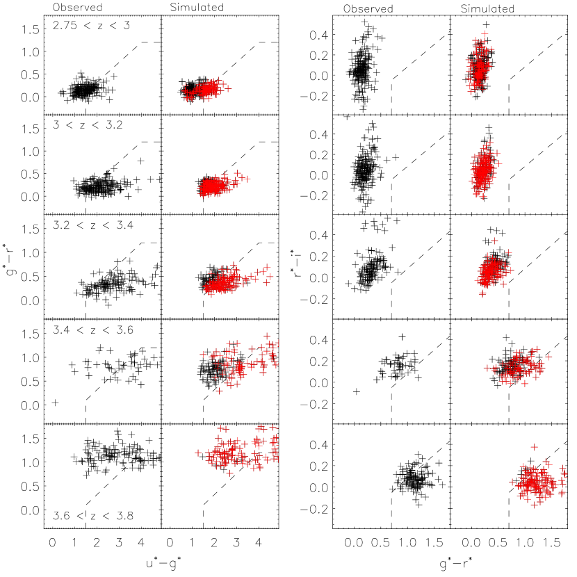
Thus, we now have a mock QSO catalog with redshifts, luminosities in five bands, and hence colors. The different panels in Figure 18 show the distribution of observed (left) and simulated (right) colors in different redshift bins. The dashed lines show some of the SDSS selection cuts (the total set of selection criteria is described in Richards et al. 2002a). In the panels which show the simulated colors, fainter symbols show objects which would have been targetted for observation by the SDSS collaboration, and darker symbols show objects which the collaboration would not have observed.

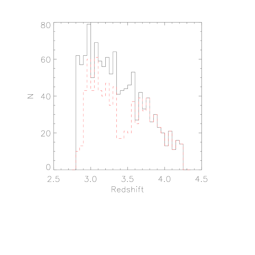
On the whole, the simulated and observed samples are rather similar, although there are significant differences around $3.2<z<3.6$, and smaller differences at $z<3$. To quantify this, Figure 19 compares the $N(z)$ distribution of the simulated complete sample (solid line) with the distribution of the subsample selected following the SDSS selected procedure (dashed line). Notice how the simulated SDSS–subsample is missing objects in the range $3.2<z<3.6$. Comparison with Figure 16 shows that the resulting mock $N(z)$ distribution is rather similar to that seen in the data, suggesting that our mock catalogs are a reasonable model of the selection effect.

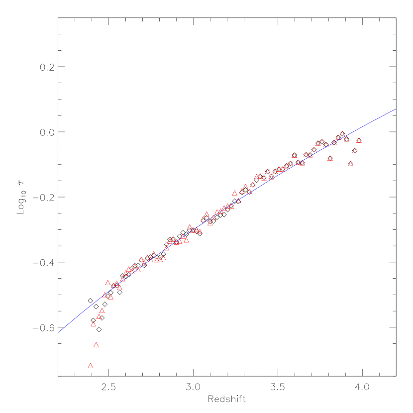
Our concern is that this selection effect may be responsible for the feature we see in $\tau_{\rm eff}(z)$ (Figure 4). To address this, Figure 20 compares $\tau_{\rm eff}(z)$ in the simulated complete sample with $\tau_{\rm eff}(z)$ in the SDSS–selected subsample. The figure shows that the evolution of $\tau_{\rm eff}$ in both cases is very similar, even in the regime in which the SDSS–selected subsample contains many fewer objects than the complete sample. This suggests that the QSO selection does not give rise to the feature we see in Figure 4.

B.2 The spectrograph

The feature in the Ly$\alpha$ forest at $z\sim 3.2$ occurs in the observed wavelength range $\lambda\sim 5000$ Å. Our measurement makes strong demands on how well the SDSS spectrograph is calibrated. The rest wavelength range $1430-1500$ Å immediately blueward of the C IV emission line of most QSO spectra is relatively flat—indeed, as described in the main text, it is from within this region that we normalize the flux in each spectrum. We used this region to test whether inaccuracies in the spectrograph could have caused the feature we detected as follows.

Figure 21: The mean transmission in the Ly$\alpha$ forest (stars; rest wavelength range $1080-1160$ Å) and the C IV forest (triangles; rest wavelength range $1430-1480$ Å) of QSOs at $2<z<3$, as a function of observed wavelength. There is no feature at $\lambda_{obs}\sim 5000$ Å in the mean C IV transmission (triangles), but there is a feature in the Ly$\alpha$ transmission (stars).

Figure 22: Mean transmission in the C IV forest (rest wavelength range $1430-1480$ Å) of QSOs at $1.75<z<2.5$, as a function of observed wavelength. Spectra were normalized by the flux redward of C IV. There is a sudden drop in the observed flux at $\lambda_{obs}<4400$ Å. The magnitude of the drop is similar to that seen in the Ly$\alpha$ forest of QSOs at $z\sim 2.8$, redshifted to the same observed wavelength. This similarity suggests that there is a problem with the spectroscopic calibrations: $\lambda_{obs}\sim 4400$ Å is close to the blue end of the spectrograph.

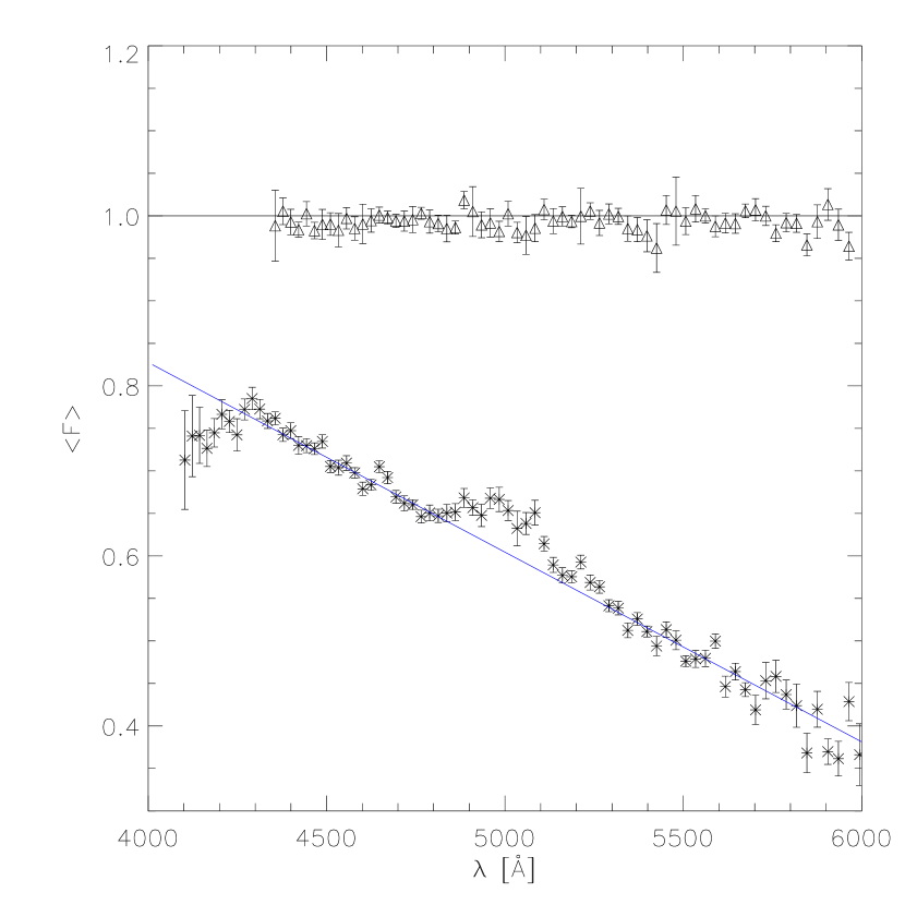
Since the wavelength region blueward of the C IV emission line lies $\sim 300$ Å redward of the Ly$\alpha$ forest, to cover the same observed wavelength range it was necessary to use a sample of QSOs at lower redshift than the sample used in this paper. Therefore, we extracted from the SDSS database 600 QSOs in the redshift interval $2<z<3$ (excluding BALs and/or low quality spectra). We normalized each spectrum by the flux in the rest wavelength range $1350-1370$ Å(the region blueward of Si IV). We then fit a continuum as described in the main text, and measured the mean transmission relative to this continuum in the wavelength range $1440-1480$ Å, what we will call the C IV forest. Figure 21 compares the mean transmission versus observed wavelength in the Ly$\alpha$ forest (stars) and the C IV forest (triangles). Notice that there is no feature in the C IV forest. This indicates that calibration problems are not responsible for the feature we see in the Ly$\alpha$ forest.

We stated in the main text that flux calibration problems near the blue end of the spectrograph limit the redshift range over which we can study the Ly$\alpha$ forest. To illustrate the problem, we first selected 1000 QSOs at $1.75<z<2.5$. We then calibrated each spectrum as follows. Since C IV is at the blue end of the spectrum for the lower redshift QSOs, the region blueward of Si IV (the restframe wavelength $1350-1370$ Å) is not measured, and so it cannot be used to calibrate. The Vanden Berk et al. (2001) composite spectrum shows that the closest region redward of C IV which is not contaminated by emission lines is far away—at about 5000 Å in the restrame! On the other hand, although the region just redward of C IV is contaminated by emission, it is relatively featureless, and it does not appear to change very much in the redshift range $1.75<z<2.5$. Therefore, we used this region to calibrate the low redshift spectra, and we then measured the mean transmission in the C IV forest. Figure 22 shows that the mean transmission is relatively constant redward of $\lambda_{obs}\sim 4400$ Å; it is less than unity because the region just redward of C IV contains more flux than the region just blueward of C IV (cf. Figure 14). However, the transmitted flux decreases by slightly more than ten percent between 4400 Å and 4000 Å.

A drop of slightly more than ten percent is also seen in the Ly$\alpha$ forest at these same wavelengths. There is no reason to believe that the Ly$\alpha$ optical depth at $z_{\alpha}\sim 4400/1215.67-1$ should be correlated with the C IV optical depth at $z\sim 2$, so the occurence of the feature almost certainly reflects a problem with the spectroscopic calibrations.

Appendix C A skewed distribution for $\tau$

Figure 23: Comparison of the mean (solid lines) and median (dotted lines) values of $\tau_{\rm eff}$ in the wavelength range $1080-1160$ Å as a function of redshift. From bottom to top, dotted curves show $\tau_{\rm eff}$ computed splitting the Ly$\alpha$ forest using different bin sizes: 150 kms^-1, 300 kms^-1, 450 kms^-1, 600 kms^-1, and 750 kms^-1. The mean values are insensitive to the bin size, whereas the median is strongly affected—this is a signature of the fact that the scatter around the mean is asymmetric.

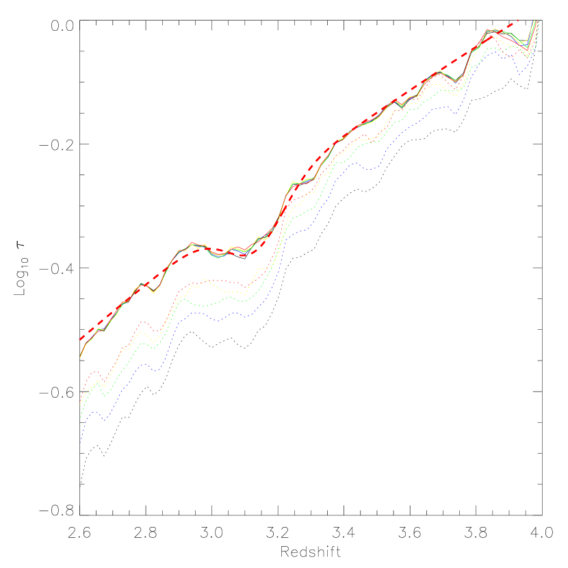
In the main text we showed that our estimate of the mean transmission did not depend strongly on the length of the segments over which the measurement was averaged, provided this length was small. Although the bin size is not important for mean statistics, the bin size does matter for median statistics.

The solid curves in Figure 23 show the evolution of $\tau_{\rm eff}$ computed using $\langle\bar{F}\rangle$, the mean value of $\bar{F}$, as the bin size is increased from 150 kms^-1 (bottom), to 300 kms^-1, 450 kms^-1, 600 kms^-1, and 750 kms^-1 (top). The curves are indistinguishable from each other, illustrating that our results do not depend on the size of the bin. The dotted lines show the same, but for the evolution of $\tau_{\rm eff}$ computed using the median value of $\bar{F}$ rather than the mean. The Figure shows that, in this case, the bin size does matter — the estimate from the median becomes increasingly similar to that from the mean as the bin size increases. Nevertheless, the $\tau_{\rm eff}$ does show a feature at $z\sim 3.2$, whatever the smoothing scale.

That the median optical depth is smaller than the mean is a consequence of the well known fact that the distribution of flux decrements is skewed. Smoothing makes the fluxes in different pixels similar, so the median and mean values become increasingly alike as the smoothing scale is increased.

References

- (1) Boksenberg, A. 1998, Structure and Evolution of the IGM from QSO Absorption Line Systems, eds. P. Petitjean & S. Charlot (Paris: Ed. Frontières), 85
- (2) Croft, R. A. C., Weinberg, D. H., Katz, N. & Hernquist, L. 1997, ApJ, 488, 532
- (3) Francis, P. J., Hewett, P. C., Foltz, C. B. & Chaffee, F. H. 1992, ApJ, 398, 476
- (4) Frieman, J., et al. 2002, in preparation
- (5) Fukugita, M., Ichikawa, T., Gunn, J. E., Doi, M., Shimasaku, K., & Schneider, D. P. 1996, AJ, 111, 1748
- (6) Gaztañaga, E. & Croft, R. A. C., 1999, MNRAS, 309, 885
- Gunn & Peterson (1965) Gunn, J. E. & Peterson, B. A. 1965, ApJ, 142, 1633
- (8) Gunn, J. E. et al. 1998, AJ, 116, 3040
- (9) Heap, S. R., Williger, G. M., Smette, A., Hubeny, I., Sahu, M. S., Jenkins, E. B., Tripp, T. M., & Winkler, J. N. 2000, ApJ, 534, 69
- (10) Hernquist, L., Katz, N.., Weinberg, D.H., Miralda-Escudé, J., 1996, ApJ, 457, L51
- (11) Jenkins, E. B., Ostriker, J. P. 1991, ApJ, 376, 33
- (12) Kim, T., Cristiani, S., & D’Odorico, S. 2002, A&A, 383, 747
- (13) Kriss, G. A. et al. 2001, Science, 293, 1112
- (14) Kulkarni, V. P., Huang, K.-L., Green, R. F., Bechtold, J., Welty, D. E., & York, D. G. 1996, MNRAS, 279, 197
- (15) Lupton, R., Gunn, J. E., Ivezić, Z., Knapp, G. R., & Kent, S. 2001, in ASP Conf. Ser. 238, Astronomical Data Analysis Software and Systems X, ed. F. R. Harnden, Jr., F. A. Primini, and H. E. Payne (San Francisco: Astr. Spc. Pac.), p. 269 (astro-ph/0101420)
- (16) Lynds, R. 1971, ApJL, 164, 73
- (17) McDonald, P., Miralda-Escudé, J., Rauch, M., Sargent, W. L. W., Barlow, T. A., Cen, R., Ostriker, J. P. 2000, ApJ, 543, 1
- (18) McDonald, P., Miralda-Escudé, J., Rauch, M., Sargent, W. L. W., Barlow, T. A., & Cen, R. 2001, ApJ, 562, 52
- (19) McDonald, P. & Miralda-Escudé, J. 2001, ApJ, 549, L11
- (20) Meiksin, A. 1994, ApJ, 431, 109
- (21) Oke, J. B., & Koryansky, D. G., 1982, ApJ, 255, 11
- (22) Peebles, P. J. E. 1993, Principles of physical cosmology, Princeton University Press
- (23) Press, W. H., Rybicki, G, B. & Schneider, D. P. 1993, ApJ, 414, 64
- (24) Rauch, M., Miralda-Escudé, J., Sargent, W. L. W., Barlow, T. A., Weinberg, D. H., Hernquist, L., Katz, N., Cen, R., & Ostriker, J. P. 1997, ApJ, 489, 7
- (25) Rauch, M., 1998, ARA&A, 36, 267
- (26) Reimers, D., Kohler, S., Wisotzki, L., Groote, D., Rodeiguez-Pascual, P., & Warmsteker, W., 1997, A&A, 327, 890
- (27) Richards, G. T., York, D. G., Yanny, B., Kollgaard, R. I., Laurent-Muehleisen, S. A., & Vanden Berk, D. E. 1999, ApJ, 513, 576
- (28) Richards, G. T., et al. 2002a, AJ, 123, 2945
- (29) Richards, G. T., et al. 2002b, AJ, 124, 1
- (30) Ricotti, M., Gnedin, N. Y., & Shull, J. M. 2000, ApJ, 534, 41
- (31) Sargent, W. L. W., Steidel, C. C., & Bocksenberg, A. 1989, ApJS, 69, 703
- (32) Schaye, J., Theuns, T., Rauch, M., Efstathiou, G., & Sargent, W. L. W. 2000, MNRAS, 318, 817
- (33) Schneider, D. P., Schmidt, M., & Gunn, J. E. 1991, AJ, 101, 2004
- (34) Songaila, A. & Cowie, L. L. 1996, AJ, 112, 335
- (35) Songaila, A. 1998, AJ, 115, 2184
- (36) Songaila, A. & Cowie, L. L. 2002, AJ, 123, 2183
- (37) Steidel, C. C. & Sargent, W. L. W. 1987, ApJ, 313, 171
- (38) Stoughton, C. et al. 2002, AJ, 123, 485
- (39) Theuns, T., Schaye, J., Zaroubi, S., Kim, T., Tzanavaris, P., & Carswell, B. 2002a, ApJL, 567, 103
- (40) Theuns, T., Zaroubi, S., Kim, T., Tzanavaris, P., & Carswell, R. F. 2002b, MNRAS, 332, 367
- (41) Theuns, T., Bernardi, M., Frieman, J., Hewett, P., Schaye, J., Sheth, R. K., & Subbarao, M. 2002, ApJL, 574, 111
- (42) Vanden Berk, D. E. et. al. 2001, AJ, 122, 549
- (43) York, D. G. et al. 2000, AJ, 120, 1579
- (44) Zaldarriaga, M., Hui, L., & Tegmark, M. 2001, ApJ, 557, 519
- (45) Zheng, W., Kriss, G. A., Telfer, R. C., Grimes, J. P., & Davidsen, A. F. 1997, ApJ, 475, 469
- (46) Zuo, L., & Lu, L. 1993, ApJ, 418, 601