Wind Accretion and State Transitions in Cygnus X-1

Abstract

We present the results of a spectroscopic monitoring program (from 1998 to 2002) of the H$\alpha$ emission strength in HDE 226868, the optical counterpart of the black hole binary, Cyg X-1. The feature provides an important probe of the mass loss rate in the base of the stellar wind of the supergiant star. We derive an updated ephemeris for the orbit based upon radial velocities measured from He I $\lambda 6678$. We list net equivalent widths for the entire H$\alpha$ emission/absorption complex, and we find that there are large variations in emission strength over both long (years) and short (hours to days) time spans. There are coherent orbital phase related variations in the profiles when the spectra are grouped by H$\alpha$ equivalent width. The profiles consist of (1) a P Cygni component associated with the wind of the supergiant, (2) emission components that attain high velocity at the conjunctions and that probably form in enhanced outflows both towards and away from the black hole, and (3) an emission component that moves in anti-phase with the supergiant’s motion. We argue that the third component forms in accreted gas near the black hole, and the radial velocity curve of the emission is consistent with a mass ratio of $M_{\rm X}/M_{\rm opt}\approx 0.36\pm 0.05$. We find that there is a general anti-correlation between the H$\alpha$ emission strength and X-ray flux (from the Rossi X-ray Timing Explorer All Sky Monitor instrument) in the sense that when the H$\alpha$ emission is strong ($W_{\lambda}<-0.5$ Å) the X-ray flux is weaker and the spectrum harder. On the other hand, there is no correlation between H$\alpha$ emission strength and X-ray flux when H$\alpha$ is weak. We argue that this relationship is not caused by wind X-ray absorption nor by the reduction in H$\alpha$ emissivity by X-ray heating. Instead, we suggest that the H$\alpha$ variations track changes in wind density and strength near the photosphere. The density of the wind determines the size of X-ray ionization zones surrounding the black hole, and these in turn control the acceleration of the wind in the direction of the black hole. During the low/hard X-ray state, the strong wind is fast and the accretion rate is relatively low, while in the high/soft state the weaker, highly ionized wind attains only a moderate velocity and the accretion rate increases. We argue that the X-ray transitions from the normal low/hard to the rare high/soft state are triggered by episodes of decreased mass loss rate in the supergiant donor star.

1 Introduction

Cygnus X-1 has been one of the most intensively studied X-ray sources in the sky since its discovery and identification with the O9.7 Iab supergiant star, HDE 226868 (Bolton, 1972; Webster & Murdin, 1972). This system provided the first evidence for the existence of stellar mass black holes when it was discovered to be a 5.6 day binary with a massive, unseen companion. Gies & Bolton (1986a) used the spectroscopic orbit (Gies & Bolton, 1982; LaSala et al., 1998; Brocksopp et al., 1999a), light curve (Kemp et al., 1983; Karitskaya et al., 2001), photospheric line broadening, and a range in the assumed degree of Roche-filling of the supergiant star to obtain mass estimates of $M_{\rm opt}=23-43~{}M_{\odot}$ and $M_{\rm X}=10-21~{}M_{\odot}$. Herrero et al. (1995) derived physical parameters for the visible supergiant based upon a spectroscopic analysis of the line spectrum, and they adopted a system inclination of $i=35^{\circ}$ (based upon published estimates) to arrive at mass estimates of 18 and $10~{}M_{\odot}$ for the supergiant and black hole, respectively (the derived masses scale as $\sin^{-3}i$ over the probable range of $i=30^{\circ}-40^{\circ}$; Gies & Bolton (1986a); Wen et al. (1999)). The X-ray source in Cyg X-1 is powered mainly by accretion from the strong stellar wind of the supergiant star (Petterson, 1978; Kaper, 1998). In fact, Cyg X-1 probably represents a situation intermediate between pure, spherical wind accretion and accretion by Roche lobe overflow. Observations of the optical emission lines (Gies & Bolton, 1986b; Ninkov et al., 1987) indicate that the wind departs from spherical symmetry and that there exists an enhanced wind flow (or “focused wind”) in the direction of the companion. The intense X-ray emission is believed to be produced close to the black hole in an accretion disk that emits soft X-ray photons and in a hot corona that inverse-Compton scatters low energy photons to higher energies (Liang & Nolan, 1984; Tanaka & Lewin, 1995). Ultraviolet radiation from close to the black hole has been detected through High Speed Photometer observations with the Hubble Space Telescope (Dolan, 2001). Radio jets were recently discovered in Cyg X-1 (Stirling et al., 2001; Fender, 2001) indicating a collimated outflow with a speed in excess of $0.6c$, so that Cyg X-1 joins the group of Galactic microquasars, small scale versions of active galactic nuclei (Mirabel & Rodríguez, 1999). The target is also a candidate $\gamma$-ray transient source (Golenetskii et al., 2002); the $\gamma$-rays are probably created through inverse-Compton scattering in the jets.

Cyg X-1 is generally found in either a low/hard state (the more common case of low 2-10 keV flux and a hard energy spectrum) or a high/soft state (in which the soft X-ray flux increases dramatically and the spectrum softens; Zhang et al. (1997); Zdziarski et al. (2002)). Every few years Cyg X-1 makes a transition from the low/hard to the high/soft state, and it remains in this active state for weeks to months before returning to the low/hard state. The last well documented high/soft state occurred in 1996 (Brocksopp et al., 1999b), and in 2001 September Cyg X-1 once again entered a high/soft state in which it still remains at the time of writing (2002 September). This recent transition into the high/soft state was accompanied by a sudden decrease in radio flux (Pooley, 2001) (the opposite of the radio brightening that accompanied the return to the low/hard state in 1971 and that led directly to the identification of the visible star associated with the X-ray source; Hjellming et al. (1971)). There are many theories about the causes of the transitions (Chakrabarti & Titarchuk, 1995; Poutanen et al., 1997; Meyer et al., 2000; Wen et al., 2001; Young et al., 2001; Robertson & Leiter, 2002) which generally relate to the physical conditions of the gas surrounding the black hole. For example, Esin et al. (1998) describe the transitions in terms of an advection-dominated accretion flow (ADAF) model in which the transitions are related to changes in the inner radius of the geometrically thin, optically thick, Keplerian disk. In the usual low/hard state, the inner disk radius is relatively large, but during the high/soft state the inner radius extends inwards close to the last stable orbit around the black hole. The transition to the high/soft state is generally believed to be the result of a moderate increase in the mass accretion rate.

However, there is no clear observational evidence available to support the claim of enhanced mass transfer during the high/soft state. In fact, the evidence collected so far hints that the supergiant mass loss rate may actually decline during the high/soft state. Wen et al. (1999) present a model for the X-ray light curve of Cyg X-1 during the prolonged low/hard state based upon the accumulated data from the Rossi X-ray Timing Explorer Satellite (RXTE) All Sky Monitor (ASM) instrument (see also Karitskaya et al. (2001)). They find that the decreased X-ray flux observed when the supergiant is in the foreground can be explained by the X-ray absorption caused by the wind outflow from the supergiant. However, during the high/soft state the orbital variation in X-ray flux disappears, and Wen et al. argue that the wind absorption declines because of increased photoionization of the wind by the stronger X-ray source and a decrease in the wind density (implying a factor of 2 decrease in the mass loss rate). Voloshina et al. (1997) found that the H$\alpha$ emission associated with the wind loss also declined during the 1996 high/soft state. Taken at face value, these observations suggest that the wind mass loss actually declines during a high/soft state, in contradiction to the theoretical expectations.

In this paper we report on multiple year observations of the H$\alpha$ emission line in HDE 226868 (§2) which we find to show significant long term and short term variability (§3), presumably reflecting changes in the wind close to the supergiant. The RXTE/ASM instrument has provided continuous X-ray flux measurements of the binary throughout this period, and we show that temporal variations in the X-ray flux are broadly anti-correlated with the H$\alpha$ emission strength (§4). We discuss the implications of this result, and we suggest that the state transitions may result from changes in the wind velocity that are related to the ionization state of the wind (§5).

2 Observations and Orbit

The 115 optical spectra were made from three different sites over the period from 1998 August to 2002 May, and we list in the final column of Table 1 the specific telescope and spectrograph combination associated with each observation. The majority of the spectra were obtained with the Kitt Peak National Observatory 0.9-m Coude Feed Telescope in conjunction with a program on SS 433. Details about these observations are given in Gies et al. (2002). During the observing runs in 1998 and 2000, we used the long collimator, grating B (in second order with order sorting filter OG550), camera 5, and a Ford $3072\times 1024$ CCD (F3KB) detector. This arrangement produced a resolving power, $R=\lambda/\Delta\lambda=9530$, and covered a range of 829 Å around H$\alpha$. The KPNO Coude Feed runs in 1999, however, relied upon the short collimator, grating RC181 (in first order with a GG495 filter to block higher orders), and camera 5 with the same F3KB detector, and this set up provided lower resolving power, $R=4630$, but broader spectral coverage (1330 Å). We usually obtained two consecutive exposures of 30 minutes duration and co-added these spectra to improve the S/N ratio. We also observed the rapidly rotating A-type star, $\zeta$ Aql, which we used for removal of atmospheric water vapor lines. Each set of observations was accompanied by numerous bias, flat field, and Th Ar comparison lamp calibration frames.

We also obtained in 1999 several high dispersion echelle spectra using the University of Texas McDonald Observatory 2.1-m telescope and Sandiford Cassegrain Echelle Spectrograph (McCarthy et al., 1993). The detector was a Reticon $1200\times 400$ CCD (RA2) with $27\mu$m square pixels which recorded 27 echelle orders covering the region blueward from H$\alpha$ with a resolving power of $R=42000$. The exposure times were typically 30 minutes. The observations from 2001 to 2002 were made with the University of Toronto David Dunlap Observatory (DDO) 1.9-m telescope. The DDO spectra were obtained with the Cassegrain spectrograph and a Thomson $1024\times 1024$ CCD. All but one of these spectra were made with a 1800 grooves mm^-1 grating that yielded a resolving power of $R=11200$. The exposure times were usually 20 minutes.

The spectra were extracted and calibrated using standard routines in IRAF. All the spectra were rectified to a unit continuum by the fitting of line-free regions using the IRAF task continuum (and in the case of the echelle spectra, the resulting orders were then linked together using the task scombine). The removal of atmospheric lines was done by creating a library of telluric standard spectra from each run, removing the broad stellar features from these, and then dividing each target spectrum by the modified atmospheric spectrum that most closely matched the target spectrum in a selected region dominated by atmospheric absorptions. The spectra from each run were then transformed to a common heliocentric wavelength grid. The higher resolution spectra were smoothed to the nominal, two pixel resolution of the lower resolution spectra obtained with the KPNO Coude Feed and the RC181 grating. This degradation in resolution is inconsequential for the analysis of the broad structures in H$\alpha$ that we describe here.

We discuss below the spectral variations related to orbital phase, and in order to determine an accurate ephemeris for the orbit, we decided to measure radial velocities using the photospheric line He I $\lambda 6678$. The red wing of this feature is blended with He II $\lambda 6683$, which occasionally is filled in with weak, P Cygni type emission (also observed in He I $\lambda 5876$). We measured radial velocities by fitting a Gaussian function to the central line core in order to avoid some of these problems with the line wings, but our final results are probably influenced by the varying strength of the P Cygni emission. We also measured the position of the interstellar line at 6613.56 Å in order to correct for small differences in the wavelength calibration from the different spectrographs (this line is clear of the nearby N II $\lambda 6610$ emission line of the supergiant). We measured these differences by cross-correlating the profile of the interstellar line in each spectrum with the same profile obtained at KPNO on HJD 2,451,425.8079, and the measured stellar radial velocities were adjusted according to these cross-correlation shifts. The final radial velocity measurements are listed in Table 1.

We made a solution of the orbital elements using the nonlinear, least-squares fitting program of Morbey & Brosterhus (1974). All the radial velocities were assigned the same weight in computing the solution, and we assumed a circular orbit (Gies & Bolton, 1982). A first trial solution with a fitted period resulted in an orbital period that was the same within errors as that derived by Brocksopp et al. (1999a) based upon all the available radial velocity data, and since the data used by Brocksopp et al. (1999a) span a 26 year interval, we decided to fix the period at their value, $P=5.599829\pm 0.000016$ d. We then solved for the remaining parameters: the epoch of supergiant inferior conjunction, $T$(IC), the semiamplitude, $K$, and systemic velocity, $V_{0}$. The measurements and radial velocity curve are shown in Figure 1, and our solution is compared to that of Brocksopp et al. (1999a) in Table 2. This table also lists the r.m.s. residuals from the fit, $\sigma$, the mass function, $f(m)$, and the projected component of the semimajor axis, $a_{1}\sin i$. The individual observed minus calculated residuals, $(O-C)$, and orbital phases, $\phi$, are given in Table 1. Our derived epoch is $0\fd 043\pm 0\fd 013$ later than that predicted by ephemeris of Brocksopp et al. (1999a), and we will use our new result in what follows. The semiamplitude is in good agreement with prior work (Gies & Bolton, 1982; LaSala et al., 1998; Brocksopp et al., 1999a), but the systemic velocity is somewhat low due to the subtle P Cygni emission in He I $\lambda 6678$ (which causes the absorption core to appear slightly blue-shifted). Thus, our estimate of $V_{0}$ is probably smaller than the physical systemic velocity of the binary.

3 H$\alpha$ Variability

The H$\alpha$ feature is regarded as a reliable source for the determination of the mass loss rate in luminous hot stars (Puls et al., 1996). The line appears as an absorption profile in stars with small mass loss rates, and it grows into a strong emission profile in stars with well developed winds. The emission forms by recombination, and since this process depends on the square of the gas density, the H$\alpha$ feature serves as a probe of the dense, basal wind near the stellar photosphere. The observational evidence to date demonstrates that the H$\alpha$ emission is also time variable, especially in luminous supergiants like the visible star in Cyg X-1. Kaper et al. (1998) show an example of large H$\alpha$ emission variations over the course of a few days in the O9.5 Ib star, $\zeta$ Ori, which presumably result from changes in the wind density and structure. Kaper et al. (1997) discuss several cases of cyclical variability in H$\alpha$ that is related to the rotational period of the star. The H$\alpha$ feature in Cyg X-1 appears to be cyclically variable with the orbital period (Hutchings et al., 1974, 1979; Ninkov et al., 1987; Sowers et al., 1998), but these earlier investigations were too limited in time coverage to reveal the large variations that can occur that are unrelated to orbital phase. Both kinds of variability offer important clues about the structure and density of the wind outflow that is the ultimate source of the accretion fed X-ray luminosity.

The H$\alpha$ profiles in Cyg X-1 are often complex in appearance, and we decided to begin our analysis by measuring the overall emission strength through a simple numerical integration of the line intensity (including both emission and absorption portions). This equivalent width, $W_{\lambda}$, was measured over a 40 Å range centered on H$\alpha$, and our results are listed in the fifth column of Table 1. The measurement errors can be estimated from the values obtained during the final KPNO Coude Feed run when Cyg X-1 was usually observed twice each night. Since the emission variations generally occur on longer time scales (days), the scatter within a night mainly reflects measurement errors. The mean of the differences in equivalent width within each night indicate typical measurement errors of $\pm 0.08$ Å.

We find that the equivalent width varied from $+0.3$ Å (absorption stronger than emission) to $-1.7$ Å (emission much stronger than absorption) over the course of our observations (see Fig. 10 below). The variations have both a long term component (significant differences between the mean equivalent widths of the individual observing runs) and a rapid component (large night-to-night changes). The emission generally weakened between 1998 and 2002. A periodogram search indicated a possible small amplitude variation with a period of $156\pm 8$ d, which is similar to the long X-ray and radio period of $142\pm 7$ d found by Brocksopp et al. (1999b). However, our sampling is too fragmentary to characterize accurately variations on timescales of months, and we focus here on profile variations that are related to orbital phase. We found that these were best seen when the profiles were grouped into samples with similar H$\alpha$ equivalent width. Figures 2, 3, and 4 illustrate the profiles as a function of heliocentric radial velocity and orbital phase for times between 1998 and 2000 of strong ($W_{\lambda}<-0.9$ Å), moderate ($-0.9<W_{\lambda}<-0.4$ Å), and weak ($W_{\lambda}>-0.4$ Å) H$\alpha$ emission, respectively. Figure 5 shows the same for the DDO spectra (2001 – 2002), obtained during the high/soft X-ray state when the H$\alpha$ emission was generally weak. The upper panel in each diagram shows the observed profiles while the lower panel is a gray-scale representation of the profiles made through a linear interpolation in orbital phase. The thick line in Figure 4 depicts the H$\alpha$ profile observed on HJD 2,451,466.6863, just 3 hours prior to the midpoint of the recent Chandra observation of high resolution X-ray spectroscopy (Schulz et al., 2002). The emission was weak at that time, and the relatively low column density found by Schulz et al. (2002) probably results from the lower density in the wind at that epoch (or possibly from higher X-ray ionization of the wind; see §5).

Each diagram shows the orbital motion of the supergiant star as a backwards “S” curve in the grayscale image, and there is clear evidence of this orbital motion in a blue-shifted absorption and a red-shifted emission feature (perhaps best seen in the weaker emission profiles in Figs. 4 and 5). This is the characteristic P Cygni-type shape that is the hallmark of mass loss in luminous stars (Lamers & Cassinelli, 1999), and the association of this component with the wind of the supergiant in Cyg X-1 was demonstrated in earlier observations by Ninkov et al. (1987) and Sowers et al. (1998). The overall shape and intensity of the P Cygni component is comparable to that observed in other O-type supergiants (Ebbets, 1982; Kaper et al., 1998).

The next striking feature in these diagrams is the appearance of large emission features in the wings of the profiles observed near the orbital conjunction phases, $\phi=0.0$ and 0.5. These are most evident in the moderate and strong emission profiles (Figs. 3 and 2). Furthermore, we find that the central absorption component only appears at these conjunction phases in the strong emission case (Fig. 2). The light curve solutions for Cyg X-1 (Gies & Bolton, 1986a) indicate that the supergiant is close to filling its critical Roche surface, and in such a situation the wind is predicted to develop enhanced mass outflow in the directions opposite and especially towards the black hole companion (the focused stellar wind model of Friend & Castor (1982)). We suggest that in the strong emission case the wind is substantially enhanced along the axis joining the stars and that at the conjunction phases we see the resulting emission with the largest values of projected radial velocity. These streams are also seen in partial projection against the disk of the star at the conjunctions (which creates the strong absorption seen then) while at other phases the emission is seen projected against the sky, resulting in an emission filling of the absorption core. The presence of clumps in the stream flowing towards the black hole may partially explain the temporal variations we observe and the prevalence of X-ray dips found near phase $\phi=0.0$ (Balucinska-Church et al., 2000; Feng & Cui, 2002).

All the sets of profiles show some evidence of very blue-shifted absorption near and shortly following $\phi=0.5$, supergiant superior conjunction. At this orientation we view the focused outflow in the foreground, and we suggest that the blue-shifted absorption forms in the lower density, high latitude part of the flow we see projected against the stellar disk while the lower velocity blue-shifted emission originates in the denser equatorial part of the flow that is mainly projected against the sky. If we assume that the outflow velocity is the same in both the equatorial and our direction at $\phi=0.5$, then the emission component radial velocity is equal to $\sin i$ times the absorption component radial velocity (where $i$ is the orbital inclination). For $V_{r}({\rm abs.})=-380\pm 50$ km s^-1 and $V_{r}({\rm em.})=-190\pm 30$ km s^-1, we derive an inclination of $i=30^{\circ}\pm 7^{\circ}$, which is consistent with the range of values derived from the light curve analysis ($i=28^{\circ}-38^{\circ}$; Gies & Bolton (1986a)) and with the best fit model for X-ray light curve ($i=10^{\circ}-40^{\circ}$; Wen et al. (1999)). The assumption of equal outflow velocities in these two directions is probably not fully valid. For example, Friend & Castor (1982) find that the wind outflow is faster at high latitudes than in the high density equatorial domain, so our estimate of the inclination is probably a lower limit.

The other important feature in the profile figures is the appearance of a blue-shifted emission component near $\phi=0.25$. This emission component was also found in earlier observations, and it could originate in the focused wind flow (Ninkov et al., 1987; Sowers et al., 1998) and/or in high density gas near the black hole (Hutchings et al., 1974, 1979). In our earlier study of H$\alpha$ (Sowers et al., 1998), we presented a simplified scheme to isolate this moving component of emission based upon a Doppler tomography algorithm. The basic assumption is that each profile represents the sum of a spectral component that moves with the established radial velocity curve of the supergiant (the P Cygni component discussed above) and a second component that moves with a sinusoidal radial velocity curve parameterized by a semiamplitude, $K_{\rm em}$, and an orbital phase of radial velocity maximum, $\phi_{0}$. The tomography algorithm then uses an iterative corrections scheme (Bagnuolo et al., 1994) to reconstruct the spectral line profiles for each component. We performed tomographic reconstructions over a grid of possible $K_{\rm em}$ and $\phi_{0}$ values to find a solution that minimized the differences between the observed and reconstructed composite profiles. Since we now have nearly an order of magnitude more spectra than presented in Sowers et al. (1998), we have repeated this procedure with one key difference. We showed above that the conjunction phase profiles have shapes that are dominated by enhanced outflow along the axis joining the stars, and this part of the emission will appear broader at conjunctions than at other phases. Rather than introducing a third component with phase variable width, we decided to include only the non-conjunction phase observations ($\phi=0.1-0.4$ and $0.6-0.9$) in which the emission contributions from the axial outflow will be narrow and more concentrated towards the line center (reducing any confusion with the moving component seen blue-shifted near $\phi=0.25$).

The results of our tomographic grid search for the parameters of the moving component are illustrated in Figure 6 in a plot of the root-mean-square (rms) residuals of the reconstruction fits. There are three regions in the parameter space that offer plausible solutions (and all make comparably good fits). We show the reconstructed profiles for each set of parameters in Figure 7. The first, and in our opinion most plausible, solution (marked “A”) occurs for $\phi_{0}=0.79\pm 0.04$ and $K_{\rm em}=218\pm 30$ km s^-1 (solid line). The reconstructed profiles show a well developed P Cygni profile for the component moving with the supergiant, while the second component is a single emission peak that moves with a large but approximately anti-phase motion (probably associated with gas near the black hole; see below). This radial velocity curve is shown as an “S” curve in the grayscale images of Figures 2 – 5.

A second solution (marked “B”) is found near $\phi_{0}=0.81\pm 0.06$ and $K_{\rm em}=56\pm 30$ km s^-1 (dotted line), and in this case the anti-phase moving component (right hand panel) is broader and double-peaked. This is close to the solution advocated in Sowers et al. (1998) ($\phi_{0}=0.86$ and $K_{\rm em}=68$ km s^-1) for which the Doppler shifts resemble those observed in the He II $\lambda 4686$ emission line (Gies & Bolton, 1986b; Ninkov et al., 1987). Nevertheless, the adoption of this solution for the moving component in H$\alpha$ is problematical. First, the double-peaked structure of the reconstructed moving component suggests that it is a numerical artifact of a forced solution in which the slower moving emission is compensating for deeper blue absorption in the supergiant component. Second, the enhanced axial outflow discussed above is not treated in this simple two-component approach, and this emission will tend to favor low velocity amplitude solutions (indeed, if the conjunction phase profiles are included in the reconstructions, this solution becomes more favorable). For both of these reasons, we believe this second, low velocity solution is untenable.

The final solution (marked “C”) is another numerical artifact in which the moving component moves in phase with the supergiant but with a higher velocity ($\phi_{0}=0.23\pm 0.05$ and $K_{\rm em}=185\pm 50$ km s^-1, dashed line). In this case, the moving component is a complex absorption line that modulates a double-peaked emission profile for the supergiant. We can rule out this last solution since there is almost certainly no physical scenario consistent with such properties.

The simple, two-component model for the H$\alpha$ profiles suggests that the feature results from wind loss from the supergiant (the primary’s P Cygni profile) and gas emission with an anti-phase radial velocity curve. We can use the derived kinematical parameters of the second component to explore its location in the system. The orbital geometry is sketched in Figure 8 in which we plot the system dimensions assuming that the supergiant is close to Roche filling (Gies & Bolton, 1986a). The projected radial velocity vector derived for the moving component is the sum of an orbital velocity vector (dependent on location in the system) and a possible gas flow vector. The two simplest possibilities for these vector combinations are shown in the right side of the diagram. In the first case, we assume that the emitting gas cloud is centered along the axis joining the stars and that a small vector component of gas flow from the supergiant to the black hole is responsible for the slight phase shift of the emission. This might correspond, for example, to high density gas from the focused wind encountering the disk around the black hole. Then, the black hole will be situated close to or somewhat beyond this emission location, implying a mass ratio of $q=M_{\rm X}/M_{\rm opt}\leq K_{\rm opt}/(K_{\rm em}\sin(-\phi_{0}))$. On the other hand, if we assume that the observed motion is entirely due to orbital motion, then the emission source is located slightly off axis, trailing the black hole. This could correspond to the location of a photoionization wake (Blondin et al., 1990) or a stream - disk interaction zone. The minimum disk radius estimate in the latter case would place the black hole at a position consistent with $q=(K_{\rm opt}\sin(-\phi_{0}))/K_{\rm em}$. All these possibilities suggest $q\approx 0.36\pm 0.05$, which is consistent with the range of mass ratios admitted by the light curve solutions (Gies & Bolton, 1986a), but which is lower than the estimate derived from spectroscopic analysis of the supergiant by Herrero et al. (1995).

If the moving emission component does originate in gas accreted near the black hole, then it is important to determine how the emission flux varies as the wind of the supergiant varies. We illustrate in Figure 9 the reconstructed spectra of the supergiant and moving spectral components for the same four groupings of emission equivalent width shown earlier in Figures 2 – 5. We see that there is a reasonably good correlation between the strength of the supergiant P Cygni emission (related to the wind mass loss rate) and the strength of the moving emission component (presumably related to the gas accreted by the black hole). We will return to the issue of wind accretion in §5.

4 Correlated X-ray Variability

The H$\alpha$ emission and associated stellar wind variations could be related to the X-ray flux variations, since the wind is probably the main source of material accreted by the black hole. Here we investigate the temporal variations through a comparison of the H$\alpha$ equivalent width with the X-ray flux observed with the RXTE/ASM instrument (Levine et al., 1996). The ASM records the X-ray flux in three bands (1.5 – 3 keV, 3 – 5 keV, and 5 – 12 keV), and we begin by plotting the daily average of the low energy band flux with the H$\alpha$ equivalent width in Figure 10. Our first runs occurred during the low/hard X-ray state when the soft X-ray flux was small. However, the observations made near HJD 2,451,896 correspond to a time of X-ray flaring, while the DDO runs cover the recent, extended high/soft state of Cyg X-1. The general trend appears to be an anti-correlation between $W_{\lambda}$(H$\alpha$) and the soft X-ray flux, and this same relationship is also found in some of the rapid variations. Figure 11 shows a detailed view of the co-variations observed during the third run in 1999, this time depicting the higher time resolution, dwell by dwell, X-ray fluxes. The H$\alpha$ emission strength shows a general night-to-night trend, which was interrupted during one night (HJD 2,451,426.8) when the emission dropped significantly. We see that a small X-ray flare occurred at the same time as the H$\alpha$ decrease. Figure 12 shows an example of the reverse trend observed during our run with the best time coverage from 2000 December. Here we see that the local maximum in H$\alpha$ emission strength occurred at nearly the same time as a well documented minimum in soft X-ray flux (HJD 2,451,898.6). There appear to be no obvious time lags between the H$\alpha$ and X-ray events, although our time resolution is limited by the near diurnal sampling of the H$\alpha$ observations.

We show the nature of the anti-correlation in all three X-ray bands in Figure 13. Here we have made a linear time interpolation in the dwell by dwell X-ray fluxes in order to make the best approximation of the flux values at the specific times of the H$\alpha$ observations. Note that the X-ray flux varies significantly on timescales shorter than dwell by dwell sampling rate (median interval of $\approx 0.8$ hours) and that the X-ray and optical observations are often non-contemporaneous, so that our time-interpolation estimate of the X-ray flux may have large errors. The DDO observations made during the high/soft state are plotted as diamonds while all the earlier measurements are shown as plus signs. These plots show that whenever we observed the H$\alpha$ emission to be stronger than $W_{\lambda}<-0.5$ Å, the X-ray flux was relatively low (especially in the lower energy bands). On the other hand, when the H$\alpha$ emission was weaker than this value, the X-ray flux appeared to vary over a wide range nearly independent of $W_{\lambda}$. We show a spectral hardness ratio in Figure 14 which confirms the impression that the X-ray spectrum is generally harder when the H$\alpha$ emission is stronger. These trends were first observed by Voloshina et al. (1997) (based on data obtained during the 1996 high/soft state), and they also find confirmation in an important long term monitoring program of H$\alpha$ made at the Crimean Astrophysical Observatory (A. E. Tarasov 2002, private communication).

5 Discussion

Our results indicate that X-ray flux appears to be related to the state of the wind (as observed in the H$\alpha$ emission strength). When the H$\alpha$ emission is strong the X-ray flux is consistently low, but when the emission is relatively weak the X-ray flux can cover a wide range in values. There are three processes that can potentially explain these observations: (1) X-ray photoionization of the wind leading to a decrease in H$\alpha$ emissivity; (2) wind-related changes in column density towards the X-ray source; and (3) variations in wind strength that result in changes in accretion rate. Here we argue that all three processes are required to help explain our results and that changes in the wind accretion rate may trigger the X-ray transitions in Cyg X-1.

The first possible explanation is that increased X-ray emission leads to heating of the wind and a corresponding decrease in H$\alpha$ emissivity (Brocksopp et al., 1999b). van Loon et al. (2001) show how the X-ray ionization of the wind in the low/hard state causes orbital variations in the ultraviolet P Cygni lines formed in the wind (e.g., the Hatchett-McCray effect; Hatchett & McCray (1977)). The X-ray ionization effects become more severe in the high/soft state, and Wen et al. (1999) describe how the wind absorption effects decrease significantly in such highly ionized conditions. Hydrogen is expected to be nearly fully ionized in the base of the wind irrespective of the X-ray state, but if the gas is heated by an elevated soft X-ray flux, then the H$\alpha$ emissivity will drop ($\propto T^{-1.2}$; Richards & Ratliff (1998)).

The best evidence for ionization-related variability is the reduction in H$\alpha$ equivalent width we observed during the mini-flare of X-ray flux around HJD 2,451,426.8 (Fig. 11). The increase in soft X-ray flux and reduction in H$\alpha$ occurred more-or-less simultaneously (within the time resolution of the data), as expected for the small light-travel time between the X-ray source and the facing hemisphere of the supergiant ($\approx 54$ s). On the other hand, the characteristic wind crossing time between components is approximately 10 hours, and our data, although sparse in time coverage, does not indicate any time lag of this order between the H$\alpha$ and X-ray variations. This event occurred near orbital phase $\phi=0.77$, and the two spectra we obtained then show H$\alpha$ profiles with unusually deep absorption cores (see Fig. 4) compared to observations on the preceding and following nights. At this orientation the wind between the stars was moving tangentially to our line of sight and the emission from this region, if present, would have filled in the line core. However, if this inner region was significantly photoionized by the X-ray mini-flare, then the residual emission in the line core would have vanished to produce the deeper absorption core. Thus, the timing and line properties of this event suggest it was caused by X-ray photoionization.

On the other hand, there are several lines of evidence that X-ray photoionization is not the dominant cause of the H$\alpha$ variations. First, we would expect the anti-correlation between H$\alpha$ emission and X-ray flux to be better defined than exhibited in Figure 13 if X-ray photoionization drove the emission variations (although the scatter may be partially the result of the poor time resolution and poor overlap of the H$\alpha$ and X-ray observations). There are several examples (especially during the X-ray low/hard state) where we observed large excursions in the H$\alpha$ emission while the X-ray flux was essentially constant (Fig. 10). Second, if X-ray photoionization significantly altered the H$\alpha$ emissivity of the gas above the hemisphere facing the X-ray source, then we should observe changes in the shape of the supergiant’s P Cygni component with orbital phase. The variations would be largest in the high/soft X-ray state and would result in decreased blue absorption near $\phi=0.5$ and decreased red emission near $\phi=0.0$. The spectra observed in the high/soft X-ray state (Fig. 5) show that the predicted changes may be present but are relatively minor in nature. Third, we find evidence of large scale variations in the H$\alpha$ emission that forms in the X-ray shadow above the hemisphere facing away from the X-ray source where no X-ray photoionization should occur. This region in the wind is best isolated in the radial velocity distribution of the emission near orbital phase $\phi=0.5$ when this backside outflow is the dominant contributor to the red-shifted peak of the P Cygni profile. However, given the probable low orbital inclination, this part of the profile also includes some contributions from the X-ray illuminated hemisphere. We show in Figure 15 the red peak emission height for spectra obtained near this phase plotted against X-ray flux. These diagrams show that the strength of the emission component from the X-ray shadow region is generally independent of the X-ray flux level in both the low/hard (plus signs) and high/soft (diamonds) X-ray states, as expected for an emitting region sheltered by the supergiant. In contrast, we show in Figure 16 the peak intensity of the blue emission peak isolated near orbital phase $\phi=0.25$ that displays evidence of an anti-correlation between H$\alpha$ emission and X-ray flux as expected for irradiated gas close to the black hole (§3). The large range in the strength of the H$\alpha$ emission from the X-ray shadow region suggests that variations are caused by factors other than changes in X-ray photoionization. Since the emission strength is very sensitive to gas density ($\propto n^{2}$), we conclude that the main source of the H$\alpha$ emission variations is the fluctuation in basal wind density rather than ionization state.

If the H$\alpha$ variations primarily reflect changes in wind density close to the supergiant, then it is possible that the X-ray flux is partially modulated by the changing absorption in the stellar wind (particularly important for soft X-rays). We doubt that wind absorption plays a major role in explaining the general anti-correlation between H$\alpha$ and X-ray emission because the scatter in their temporal variations (Fig. 13) is much larger than we would expect for a direct cause-and-effect relationship. Furthermore, the amplitude of the wind density fluctuations implied by the H$\alpha$ changes is too small to explain the range in X-ray variability. Wen et al. (1999) show that the X-ray light curve can be explained by the changing column density of the line of sight to the black hole as we peer through different portions of the supergiant’s wind (strongest absorption at supergiant inferior conjunction, $\phi=0.0$). Their ASM 1.5 – 3 keV orbital light curve for the low/hard state shows a 25% decrease at $\phi=0.0$ relative to $\phi=0.5$. Balucinska-Church et al. (2000) also studied the variation in column density with orbital phase, and they suggest that the orbital modulation in X-ray flux corresponds to a fluctuation of $6-10\times$ in column density (depending on the assumed ionization of the wind). However, the observed variations in the emission strength generally indicate column density changes of a factor of $<2$ (see below). Wind column density changes of this order are too small to account for the large changes in X-ray flux. Thus, wind absorption variations are insufficient to explain the general anti-correlation between the H$\alpha$ emission strength and X-ray flux. Nevertheless, we might expect the wind absorption processes to appear most prominent near inferior conjunction of the supergiant when the X-ray light curve attains a minimum and a peak occurs in the frequency of rapid X-ray dips (Wen et al., 1999; Balucinska-Church et al., 2000; Feng & Cui, 2002). It is noteworthy in this regard that the case of the simultaneous H$\alpha$ maximum and X-ray flux minimum shown in Figure 12 did indeed occur near this phase (at $\phi=0.02$).

If we ignore the effects of X-ray ionization on the H$\alpha$ emissivity, then we can make an approximate estimate of how the wind mass loss rate and density vary as a function of the H$\alpha$ emission strength (Puls et al., 1996). Herrero et al. (1995) show predictions of how the H$\alpha$ profile will vary as a function of mass loss rate (see their Fig. 4), and we measured the equivalent widths of their profiles to calibrate the mass loss rate as a function of H$\alpha$ equivalent width (prorated to their final estimate of mass loss rate for the time of their observations, $3.0\times 10^{-6}$ $M_{\odot}$ y^-1). The functional fit in this case is

$$-\dot{M}=(1.85-1.01~{}W_{\lambda}-0.04~{}W_{\lambda}^{2})~{}\times 10^{-6}~{}M_{\odot}~{}{\rm y}^{-1}.$$ (1)

We grouped our equivalent width data according to the X-ray state at the time of observation (setting aside the results obtained near HJD 2,451,896 that may correspond to a “failed transition”), and the mean equivalent width for each group yields mass loss rates of $(2.57\pm 0.05)\times 10^{-6}$ and $(2.00\pm 0.03)\times 10^{-6}$ $M_{\odot}$ y^-1 for the low/hard and high/soft states, respectively (the quoted errors are based on the standard deviation of the mean and do not include the larger errors associated with the calibration of the $W_{\lambda}-\dot{M}$ relationship and with our neglect of the multiple component nature of the H$\alpha$ emission). This suggests that the mass loss rate is $\approx 22\%$ lower during the rare high/soft state compared to the more common low/hard state. Since this calculation ignores the X-ray photoionization that may be more important in the high/soft state and since photoionization will decrease H$\alpha$ emission strength, our estimate for the mass loss rate during the high/soft state is best regarded as a lower limit. Nevertheless, the general decrease in wind strength during the high/soft state is also observed in the emission from the X-ray shadow region (Fig. 15) that should be relatively free from the effects of photoionization. We find that the mean residual emission intensity of the red peak near phase $\phi=0.5$ is $0.139\pm 0.008$ and $0.114\pm 0.006$ for the low/hard and high/soft states, respectively. Wen et al. (1999) also found that the wind mass loss rate is lower in the high/soft state based upon their analysis of the X-ray orbital light curve.

Taken at face value, our results present a paradox: the X-ray flux decreases when the wind mass loss rate increases. We suggest that the resolution of this quandary lies in how the wind velocity changes with wind ionization state (originally proposed by Ho & Arons (1987) and developed in more physical terms by Stevens (1991)). When the wind mass loss rate is high, the wind density is also proportionally high, and therefore the X-ray ionization effects on the wind are confined to the region close to the black hole since the size of the surrounding ionized region depends on wind density as $n^{-1}$ (Stevens, 1991; van Loon et al., 2001). Most of the wind volume surrounding the star will contain the many important ions that propel the radiative driving of the wind, so that it reaches a terminal velocity of approximately 2100 km s^-1 (Herrero et al., 1995). However, the wind flow close to the black hole will become ionized, and these advanced ionization states will generally have transitions at frequencies much higher than the peak of the stellar flux distribution. Consequently there are fewer absorbing transitions at frequencies where the stellar flux is concentrated and radiative driving of the wind becomes less effective. Stellar wind gas leaving the part of the supergiant facing the X-ray source will be accelerated by radiative driving, reaching a significant fraction of the terminal velocity before crossing the distant ionization boundary (Stevens, 1991). Models of wind accretion by the black hole suggest that the mass accretion rate is proportional to $\dot{M}/v^{4}$ (Bondi & Hoyle, 1944; Lamers et al., 1976; Stevens, 1991), and since the flow velocity $v$ is relatively large, only modest mass accretion occurs. It is easy to imagine that some of the outflow from the supergiant to the black hole bypasses the black hole altogether, and absorption by the gas beyond the black hole could explain the presence of a secondary minimum in the low/hard state X-ray light curve at orbital phase $\phi=0.5$ (Karitskaya et al., 2001).

However, when the mass loss rate drops, the X-ray ionization zone will become larger because of the reduced wind density. The dominant ions that provide the resonant transitions that in turn drive the stellar wind will disappear with increased ionization, and the wind outflow will experience only a modest acceleration and reach a speed of just a few hundred km s^-1 (before the flow dynamics become dominated by the gravitational acceleration of the black hole). This altered outflow will be denser and slower in the vicinity of the black hole, and since the accretion rate varies as $\dot{M}/v^{4}$, the overall accretion rate will increase significantly because of the slower outflow (and despite a real decline in $\dot{M}$).

If this basic scenario is correct, then transitions from the low/hard to the high/soft state are triggered when the supergiant undergoes an episode of reduced mass loss. Stevens (1991) demonstrates that the decrease in the wind force multiplier occurs rather suddenly once a specific gas density is reached, and we would argue that this is the reason why the transitions are relatively fast and the X-ray states are bimodal. Once the transition occurs, the system tends to remain in the high/soft state because the increased accretion rate and associated larger X-ray fluxes make it easier to keep the wind in the highly ionized state (even with modest increases in mass loss rate). The line of sight to the black hole then passes through mainly ionized gas all around the orbit, and the wind absorption of the X-ray flux decreases so much that the X-ray light curve modulation vanishes (Wen et al., 1999). The increased mass accretion in this state causes the optically thick, geometrically thin (Keplerian) accretion disk to extend further inwards towards the black hole, producing more soft X-rays, while the coronal (ADAF or sub-Keplerian) region, which produces the bulk of the hard X-rays, becomes smaller, and thus the X-ray spectrum softens (Ebisawa et al., 1996; Esin et al., 1998; Brocksopp et al., 1999b). The enhanced soft X-ray flux heats the accreting gas, which reduces the H$\alpha$ emission from the accretion flow (Fig. 9, 16). It is only once the supergiant can maintain a strong mass outflow that the wind becomes dense enough to reduce the ionization effects and to create the high speeds which then lower the mass accretion rate and force the system back to the low/hard state. The long term variations in the mass loss rates of massive supergiant stars are not well documented, but there is circumstantial evidence of significant variations on time scales of years (Ebbets, 1982; Markova, 2002). Thus, we suggest that the high/soft states that occur every 5 years or so in Cyg X-1 correspond to quasi-cyclic minima in the mass loss rate of the supergiant.

Figure 1: Radial velocity curve (solid line) derived from measurements of He I $\lambda 6678$ (filled circles). Phase 0.0 is inferior conjunction of the supergiant.

Figure 2: Upper frame: Strong emission H$\alpha$ profiles ($W_{\lambda}<-0.9$ Å) as a function of heliocentric radial velocity. The profiles are arranged in order of increasing orbital phase and each is placed in the $y$ ordinate so that the continuum equals the phase of observation. Lower frame: A gray-scale representation of the profiles above. The profile at each phase is calculated by a linear interpolation between the closest observed phases (marked by arrows on the right hand side). The gray intensity is scaled between spectral intensity 0.94 (black) and 1.15 (white) here and in Figs. 3 – 5. The first and last 20% of the orbit have been reproduced at the bottom and top of the image, respectively, to improve the sense of phase continuity. The white lines show the radial velocity curves of the supergiant and anti-phase moving component.

Figure 3: Moderate emission H$\alpha$ profiles ($-0.9<W_{\lambda}<-0.4$ Å) in the same format as Fig. 2.

Figure 4: Weak emission H$\alpha$ profiles ($W_{\lambda}>-0.4$ Å) in the same format as Fig. 2. The spectrum obtained just 3 hours prior to the Chandra observation (Schulz et al., 2002) is shown as a thick line.

Figure 5: H$\alpha$ profiles obtained during the 2001–2002 X-ray high/soft state (in the same format as Fig. 2).

Figure 6: Root-mean-square residuals from the fit of a two component tomographic reconstruction. The first component is assumed to move with the orbital motion of the supergiant star while the second component is parameterized by an orbital phase of maximum radial velocity, $\phi_{0}$, and a semiamplitude, $K_{\rm em}$. The smallest residuals are shown in white, the largest in black.

Figure 7: Reconstructed spectra of the component moving with the supergiant (left panel) and the component moving with parameters than minimize the rms residuals (right panel). The three parameter sets illustrated are (A) $\phi_{0}=0.79$ and $K_{\rm em}=218$ km s^-1 (solid line), (B) $\phi_{0}=0.81$ and $K_{\rm em}=56$ km s^-1 (dotted line), and (C) $\phi_{0}=0.23$ and $K_{\rm em}=185$ km s^-1 (dashed line). The continua levels are offset for clarity by $-0.15$ and $-0.30$ for cases B and C, respectively.

Figure 8: A diagram of the system geometry as viewed from above the orbital plane. The figure of the supergiant was calculated (ignoring radiation pressure) for a mass ratio, $q=0.36$, and a primary fill-out factor, $\rho=0.97$ (see Gies & Bolton 1986a). Orbital phases are listed around the periphery. The arrow at the stellar origin indicates the projected orbital velocity while the center-of-mass position is indicated by CM. The projected velocity vectors at positions near the secondary show the observed semiamplitude $K_{\rm em}$ of the anti-phase moving component and its derived orbital and flow components for two cases discussed in the text.

Figure 9: Reconstructed spectra of the component moving with the supergiant (left panel) and the anti-phase moving component (right panel). The different plots correspond to samples for times of (from top to bottom) strong emission (Fig. 2), moderate emission (Fig. 3), weak emission (Fig. 4), and the X-ray high/soft state (Fig. 5). The continua levels are each offset by 0.10.

Figure 10: A comparison of the H$\alpha$ equivalent width with the daily average RXTE/ASM count rate in the 1.5 – 3 keV range over the entire course of our observations. The error bar in the upper panel gives the typical measurement error for $W_{\lambda}({\rm H}\alpha)$.

Figure 11: A detailed comparison of the H$\alpha$ equivalent width with the dwell RXTE/ASM count rate in the 1.5 – 3 keV range showing an emission weakening episode near an X-ray mini-flare (HJD 2,451,426.8).

Figure 12: A detailed comparison of the H$\alpha$ equivalent width with the dwell RXTE/ASM count rate in the 1.5 – 3 keV range showing an emission strengthening – X-ray weakening event near HJD 2,451,898.7.

Figure 13: The H$\alpha$ equivalent widths versus the time-interpolated dwell RXTE/ASM count rates in the 1.5 – 3 keV (top), 3 – 5 keV (middle), and 5 – 12 keV ranges (bottom). Diamonds correspond to the high/soft state data while pluses correspond to the low/hard state data.

Figure 14: The H$\alpha$ equivalent widths versus the ratio of the 5 – 12 keV to 1.5 – 3 keV band time-interpolated dwell RXTE/ASM count rates. Diamonds correspond to the high/soft state data while pluses correspond to the low/hard state data.

Figure 15: The residual intensities of the red peak of the H$\alpha$ P Cygni profile for spectra obtained near orbital phase $\phi=0.5$ versus the time-interpolated dwell RXTE/ASM count rates (in the same format as Fig. 13). This part of the H$\alpha$ emission forms in a region where X-rays are mostly blocked by the supergiant so that photoionization effects are minimized.

Figure 16: The residual intensities of the blue peak of the H$\alpha$ profile for spectra obtained near orbital phase $\phi=0.25$ versus the time-interpolated dwell RXTE/ASM count rates (in the same format as Fig. 13). This part of the H$\alpha$ emission forms in a region close to the black hole where X-ray photoionization does appear to affect the emission strength. The outlying points probably result from time interpolation of the X-ray flux in intervals when the optical and X-ray observations are non-contemporaneous.

Table 1: Radial Velocity and Equivalent Width Measurements

HJD	Orbital	$V_{r}$	$(O-C)$	$W_{\lambda}$	Observatory/Telescope/
(-2,450,000)	Phase	(km s-1)	(km s-1)	(Å)	Grating/CCD
1053.7473	0.157	0+$52.5$	0$-3.5$	$-0.73$	KPNO/0.9m/B/F3KB
1053.7687	0.160	0+$58.1$	0+$1.1$	$-0.83$	KPNO/0.9m/B/F3KB
1055.7247	0.510	00$-4.5$	0+$7.1$	$-0.91$	KPNO/0.9m/B/F3KB
1055.7830	0.520	00$-9.1$	0+$7.4$	$-0.91$	KPNO/0.9m/B/F3KB
1056.7695	0.696	0$-79.0$	0$-0.7$	$-1.57$	KPNO/0.9m/B/F3KB
1056.7908	0.700	0$-81.3$	0$-2.4$	$-1.71$	KPNO/0.9m/B/F3KB
1057.7653	0.874	0$-68.2$	0$-7.5$	$-1.53$	KPNO/0.9m/B/F3KB
1057.7864	0.878	0$-66.0$	0$-6.6$	$-1.66$	KPNO/0.9m/B/F3KB
1058.7556	0.051	0+$23.2$	0+$6.4$	$-0.71$	KPNO/0.9m/B/F3KB
1058.7766	0.055	0+$25.6$	0+$7.1$	$-0.90$	KPNO/0.9m/B/F3KB
1061.7516	0.586	0$-49.2$	0$-3.3$	$-0.73$	KPNO/0.9m/B/F3KB
1061.7733	0.590	0$-48.5$	0$-1.1$	$-0.74$	KPNO/0.9m/B/F3KB
1062.8785	0.787	0$-86.0$	0$-5.5$	$-0.96$	KPNO/0.9m/B/F3KB
1063.8615	0.963	0$-28.0$	0$-3.5$	$-1.22$	KPNO/0.9m/B/F3KB
1065.7631	0.302	0+$57.7$	0$-6.8$	$-0.56$	KPNO/0.9m/B/F3KB
1065.7846	0.306	0+$55.2$	0$-8.7$	$-0.75$	KPNO/0.9m/B/F3KB
1066.7063	0.471	00$-0.9$	0$-7.7$	$-0.72$	KPNO/0.9m/B/F3KB
1066.7276	0.475	00$-3.0$	0$-8.0$	$-0.92$	KPNO/0.9m/B/F3KB
1354.8761	0.931	0$-41.2$	0$-2.6$	$-0.39$	KPNO/0.9m/RC181/TI5
1355.8228	0.100	0+$33.5$	0$-4.1$	$-0.89$	KPNO/0.9m/RC181/F3KB
1356.7938	0.274	0+$75.5$	0+$7.7$	$-0.49$	KPNO/0.9m/RC181/F3KB
1357.6648	0.429	0+$17.8$	0$-7.7$	$-1.00$	KPNO/0.9m/RC181/F3KB
1358.8837	0.647	0$-67.2$	0+$0.0$	$-1.16$	KPNO/0.9m/RC181/F3KB
1359.7987	0.810	0$-87.7$	$-10.5$	$-1.00$	KPNO/0.9m/RC181/F3KB
1360.7959	0.988	0$-16.0$	0$-3.5$	$-0.92$	KPNO/0.9m/RC181/F3KB
1361.6782	0.146	0+$48.6$	0$-4.4$	$-1.35$	KPNO/0.9m/RC181/F3KB
1362.7495	0.337	0+$57.0$	0$-0.5$	$-0.80$	KPNO/0.9m/RC181/F3KB
1363.6586	0.500	00+$0.3$	0+$7.1$	$-1.39$	KPNO/0.9m/RC181/F3KB
1394.8165	0.064	0+$15.1$	0$-7.4$	$-0.83$	McD/2.1m/Echelle/RA2
1396.8232	0.422	0+$23.2$	0$-5.4$	$-0.96$	McD/2.1m/Echelle/RA2
1398.8853	0.790	0$-80.1$	0+$0.0$	$-0.34$	McD/2.1m/Echelle/RA2
1399.8281	0.959	0$-34.0$	0$-7.6$	+$0.00$	McD/2.1m/Echelle/RA2
1420.8900	0.720	0$-73.1$	0+$8.1$	$-0.11$	KPNO/0.9m/RC181/F3KB
1421.7939	0.881	0$-62.0$	0$-3.7$	$-0.30$	KPNO/0.9m/RC181/F3KB
1421.8155	0.885	0$-62.8$	0$-5.9$	$-0.30$	KPNO/0.9m/RC181/F3KB
1423.8200	0.243	0+$75.3$	0+$6.8$	$-0.37$	KPNO/0.9m/RC181/F3KB
1425.8079	0.598	0$-41.4$	0+$9.2$	$-0.46$	KPNO/0.9m/RC181/F3KB
1426.7688	0.770	0$-76.4$	0+$5.6$	$-0.17$	KPNO/0.9m/RC181/F3KB
1426.7920	0.774	0$-77.0$	0+$4.7$	$-0.12$	KPNO/0.9m/RC181/F3KB
1427.7710	0.949	0$-27.7$	0+$3.2$	$-0.60$	KPNO/0.9m/RC181/F3KB
1428.7417	0.122	0+$50.4$	0+$5.0$	$-0.50$	KPNO/0.9m/RC181/F3KB
1429.7366	0.300	0+$66.4$	0+$1.4$	$-0.44$	KPNO/0.9m/RC181/F3KB
1429.7576	0.303	0+$66.3$	0+$1.9$	$-0.45$	KPNO/0.9m/RC181/F3KB
1464.6959	0.543	0$-30.3$	0$-3.4$	$-0.70$	KPNO/0.9m/RC181/F3KB
1465.7047	0.723	0$-79.9$	0+$1.5$	$-0.67$	KPNO/0.9m/RC181/F3KB
1466.6863	0.898	0$-53.0$	0$-0.9$	$-0.29$	KPNO/0.9m/RC181/F3KB
1467.6950	0.078	0+$25.5$	0$-3.2$	$-0.25$	KPNO/0.9m/RC181/F3KB
1467.7170	0.082	0+$29.3$	0$-1.0$	$-0.40$	KPNO/0.9m/RC181/F3KB
1469.6884	0.434	0+$13.3$	$-10.1$	$-0.70$	KPNO/0.9m/RC181/F3KB
1469.7095	0.438	0+$15.0$	0$-6.8$	$-0.62$	KPNO/0.9m/RC181/F3KB
1491.6827	0.362	0+$43.4$	0$-7.3$	$-0.89$	KPNO/0.9m/RC181/F3KB
1492.6604	0.536	0$-25.4$	0$-1.3$	$-0.68$	KPNO/0.9m/RC181/F3KB
1493.6465	0.712	0$-86.4$	0$-6.0$	$-0.97$	KPNO/0.9m/RC181/F3KB
1494.6562	0.893	0$-60.8$	0$-6.7$	$-1.31$	KPNO/0.9m/RC181/F3KB
1495.6573	0.072	0+$23.9$	0$-2.0$	$-1.19$	KPNO/0.9m/RC181/F3KB
1496.6541	0.250	0+$74.2$	0+$5.6$	$-0.91$	KPNO/0.9m/RC181/F3KB
1497.6574	0.429	0+$27.8$	0+$2.0$	$-1.01$	KPNO/0.9m/RC181/F3KB
1817.6317	0.569	0$-42.0$	0$-3.4$	$-0.38$	KPNO/0.9m/B/F3KB
1818.6805	0.756	0$-86.9$	0$-4.4$	$-0.28$	KPNO/0.9m/B/F3KB
1819.6634	0.932	0$-37.0$	0+$1.5$	$-0.73$	KPNO/0.9m/B/F3KB
1820.6465	0.107	0+$42.3$	0+$2.2$	$-0.43$	KPNO/0.9m/B/F3KB
1821.6565	0.287	0+$68.2$	0+$1.7$	$-0.47$	KPNO/0.9m/B/F3KB
1822.6660	0.468	00+$0.8$	0$-7.4$	$-0.22$	KPNO/0.9m/B/F3KB
1823.6554	0.644	0$-63.0$	0+$3.5$	$-0.78$	KPNO/0.9m/B/F3KB
1824.6356	0.819	0$-70.5$	0+$4.9$	$-0.56$	KPNO/0.9m/B/F3KB
1890.5663	0.593	0$-45.2$	0+$3.5$	$-0.15$	KPNO/0.9m/B/F3KB
1890.5879	0.597	0$-48.5$	0+$1.7$	$-0.05$	KPNO/0.9m/B/F3KB
1891.5880	0.776	0$-83.9$	0$-2.3$	+$0.23$	KPNO/0.9m/B/F3KB
1892.5719	0.951	0$-27.9$	0+$1.8$	+$0.30$	KPNO/0.9m/B/F3KB
1892.5933	0.955	0$-24.6$	0+$3.4$	+$0.26$	KPNO/0.9m/B/F3KB
1893.6007	0.135	0+$46.7$	0$-3.0$	+$0.05$	KPNO/0.9m/B/F3KB
1893.6217	0.139	0+$48.4$	0$-2.5$	$-0.29$	KPNO/0.9m/B/F3KB
1894.5918	0.312	0+$72.4$	0+$9.5$	$-0.21$	KPNO/0.9m/B/F3KB
1894.6129	0.316	0+$73.8$	+$11.6$	$-0.24$	KPNO/0.9m/B/F3KB
1895.5601	0.485	00+$3.5$	0+$3.3$	$-0.34$	KPNO/0.9m/B/F3KB
1895.5811	0.489	00+$2.4$	0+$4.0$	$-0.37$	KPNO/0.9m/B/F3KB
1896.5645	0.664	0$-69.0$	0+$2.8$	$-0.09$	KPNO/0.9m/B/F3KB
1896.5856	0.668	0$-71.6$	0+$1.1$	+$0.06$	KPNO/0.9m/B/F3KB
1897.5610	0.842	0$-65.6$	0+$4.6$	$-0.28$	KPNO/0.9m/B/F3KB
1897.5822	0.846	0$-65.0$	0+$4.2$	$-0.35$	KPNO/0.9m/B/F3KB
1898.5674	0.022	00+$7.8$	0+$4.4$	$-0.83$	KPNO/0.9m/B/F3KB
1898.5886	0.026	00+$9.5$	0+$4.3$	$-0.87$	KPNO/0.9m/B/F3KB
1899.5713	0.201	0+$63.6$	0$-1.5$	$-0.14$	KPNO/0.9m/B/F3KB
1899.5923	0.205	0+$60.2$	0$-5.4$	$-0.33$	KPNO/0.9m/B/F3KB
1900.5674	0.379	0+$46.6$	0+$1.5$	$-0.38$	KPNO/0.9m/B/F3KB
1900.5885	0.383	0+$44.8$	0+$1.1$	$-0.34$	KPNO/0.9m/B/F3KB
1901.5718	0.558	0$-41.3$	0$-7.2$	$-0.27$	KPNO/0.9m/B/F3KB
2191.6387	0.358	0+$56.8$	0+$4.9$	$-0.43$	DDO/1.9m/831/Thomson1KB
2192.6443	0.537	0$-15.8$	0+$8.7$	$-0.41$	DDO/1.9m/1800/Thomson1KB
2193.5913	0.706	$\cdots$	$\cdots$	$-0.34$	DDO/1.9m/1800/Thomson1KB
2198.4833	0.580	$\cdots$	$\cdots$	$-0.27$	DDO/1.9m/1800/Thomson1KB
2200.4987	0.940	$\cdots$	$\cdots$	$-0.26$	DDO/1.9m/1800/Thomson1KB
2201.4713	0.114	$\cdots$	$\cdots$	$-0.27$	DDO/1.9m/1800/Thomson1KB
2202.5888	0.313	$\cdots$	$\cdots$	$-0.20$	DDO/1.9m/1800/Thomson1KB
2203.4851	0.473	$\cdots$	$\cdots$	$-0.20$	DDO/1.9m/1800/Thomson1KB
2204.7099	0.692	0$-74.8$	0+$2.8$	+$0.01$	DDO/1.9m/1800/Thomson1KB
2205.4764	0.829	0$-66.9$	0+$6.5$	$-0.21$	DDO/1.9m/1800/Thomson1KB
2205.5825	0.848	0$-66.6$	0+$2.1$	+$0.02$	DDO/1.9m/1800/Thomson1KB
2220.4714	0.507	00$-2.5$	0+$7.6$	$-0.44$	DDO/1.9m/1800/Thomson1KB
2344.9493	0.735	0$-86.1$	0$-3.9$	+$0.03$	DDO/1.9m/1800/Thomson1KB
2361.9052	0.763	0$-75.4$	0+$6.9$	$-0.47$	DDO/1.9m/1800/Thomson1KB
2371.9104	0.550	0$-31.2$	0$-0.8$	$-0.17$	DDO/1.9m/1800/Thomson1KB
2371.9291	0.553	$\cdots$	$\cdots$	+$0.17$	DDO/1.9m/1800/Thomson1KB
2376.9030	0.442	0+$10.0$	$-10.1$	+$0.14$	DDO/1.9m/1800/Thomson1KB
2382.8795	0.509	00$-6.5$	0+$4.7$	$-0.11$	DDO/1.9m/1800/Thomson1KB
2388.8805	0.581	0$-41.7$	0+$1.9$	$-0.06$	DDO/1.9m/1800/Thomson1KB
2404.6914	0.404	0+$36.6$	0+$0.7$	+$0.08$	DDO/1.9m/1800/Thomson1KB
2404.8684	0.436	0+$13.9$	0$-8.9$	$-0.13$	DDO/1.9m/1800/Thomson1KB
2410.7116	0.479	00$-2.1$	0$-5.0$	$-0.03$	DDO/1.9m/1800/Thomson1KB
2410.7443	0.485	00+$4.5$	0+$4.3$	$-0.21$	DDO/1.9m/1800/Thomson1KB
2413.7035	0.013	00+$6.1$	0+$6.7$	$-0.18$	DDO/1.9m/1800/Thomson1KB
2414.7121	0.194	0+$65.4$	0+$1.5$	+$0.02$	DDO/1.9m/1800/Thomson1KB
2414.7522	0.201	0+$65.8$	0+$0.8$	$-0.01$	DDO/1.9m/1800/Thomson1KB
2414.7836	0.206	0+$69.4$	0+$3.6$	$-0.10$	DDO/1.9m/1800/Thomson1KB
2414.8197	0.213	0+$70.7$	0+$4.2$	$-0.23$	DDO/1.9m/1800/Thomson1KB

Table 2: Circular Orbital Elements

Element	Brocksopp et al. (1999)	This Work
$P$ (d)	5.599829 (16)	5.599829
$T$(IC) (HJD)	2,441,874.707 (9)	2,451,730.449 (8)
$K_{1}$ (km s-1)	74.9 (6)	75.6 (7)
$V_{0}$ (km s-1)	$\cdots$	$-$7.0 (5)
$\sigma$ (km s-1)	$\cdots$	5.3
$f(m)$ ($M_{\odot}$)	0.244	0.251 (7)
$a_{1}\sin i$ ($R_{\odot}$)	$\cdots$	8.36 (8)

Note. — Numbers in parentheses give the error in the last digit quoted.

Figure 1:

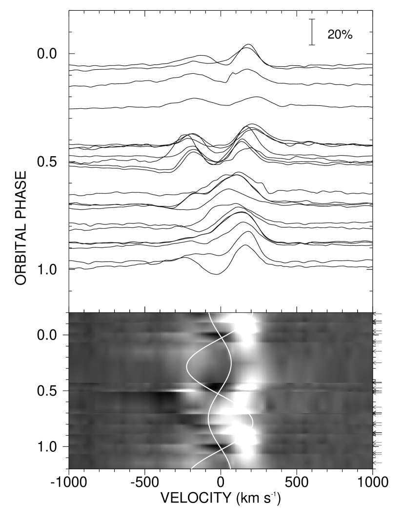
Figure 2:

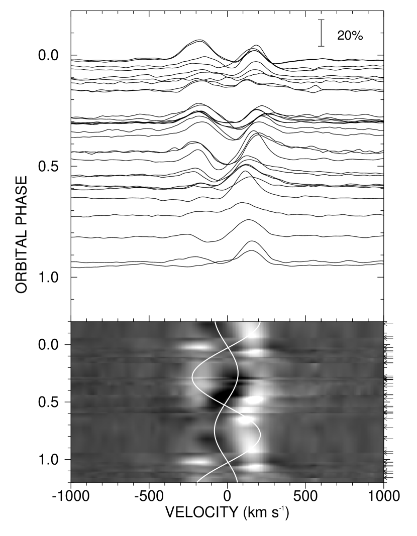
Figure 3:

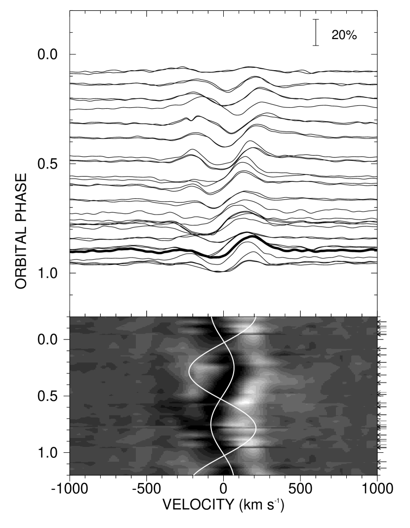
Figure 4:

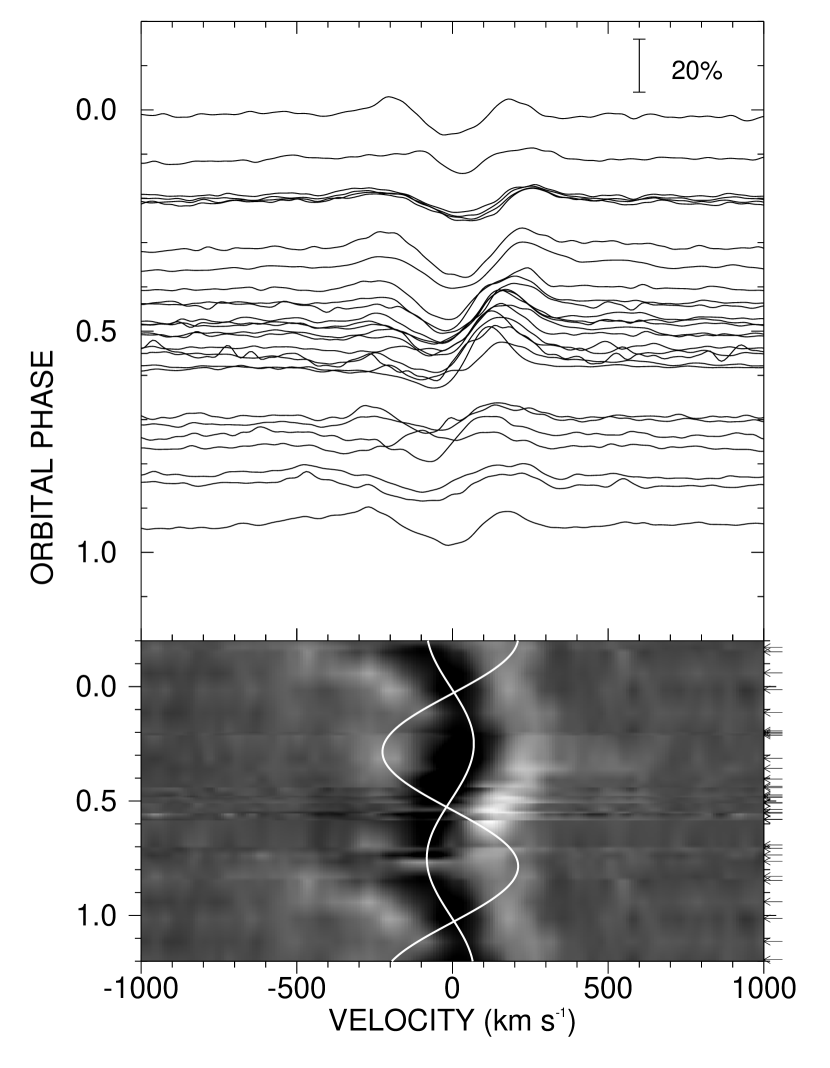
Figure 5:

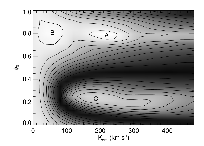
Figure 6:

Figure 7:

Figure 8:

Figure 9:

Figure 10:

Figure 11:

Figure 12:

Figure 13:

Figure 14:

Figure 15:

Figure 16:

References

- Bagnuolo et al. (1994) Bagnuolo, W. G., Jr., Gies, D. R., Hahula, M. E., Wiemker, R., & Wiggs, M. S. 1994, ApJ, 423, 446
- Balucinska-Church et al. (2000) Balucinska-Church, M., Church, M. J., Charles, P. A., Nagase, F., LaSala, J., & Barnard, R. 2000, MNRAS, 311, 861
- Blondin et al. (1990) Blondin, J. M., Kallman, T. R., Fryxell, B. A., & Taam, R. E. 1990, ApJ, 356, 591
- Bolton (1972) Bolton, C. T. 1972, Nature, 235, 271
- Bondi & Hoyle (1944) Bondi, H., & Hoyle, F. 1944, MNRAS, 104, 273
- Brocksopp et al. (1999b) Brocksopp, C., Fender, R. P., Larionov, V., Lyuty, V. M., Tarasov, A. E., Pooley, G. G., Paciesas, W. S., & Roche, P. 1999b, MNRAS, 309, 1063
- Brocksopp et al. (1999a) Brocksopp, C., Tarasov, A. E., Lyuty, V. M., & Roche, P. 1999a, A&A, 343, 861
- Chakrabarti & Titarchuk (1995) Chakrabarti, S., & Titarchuk, L. G. 1995, ApJ, 455, 623
- Dolan (2001) Dolan, J. F. 2001, PASP, 113, 974
- Ebbets (1982) Ebbets, D. 1982, ApJS, 48, 399
- Ebisawa et al. (1996) Ebisawa, K., Titarchuk, L., & Chakrabarti, S. K. 1996, PASJ, 48, 59
- Esin et al. (1998) Esin, A. A., Narayan, R., Cui, W., Grove, J. E., & Zhang, S.-N. 1998, ApJ, 505, 854
- Fender (2001) Fender, R. P. 2001, MNRAS, 322, 31
- Feng & Cui (2002) Feng, Y. X., & Cui, W. 2002, ApJ, 564, 953
- Friend & Castor (1982) Friend, D. B., & Castor, J. I. 1982, ApJ, 261, 293
- Gies & Bolton (1982) Gies, D. R., & Bolton, C. T. 1982, ApJ, 260, 240
- Gies & Bolton (1986a) Gies, D. R., & Bolton, C. T. 1986a, ApJ, 304, 371
- Gies & Bolton (1986b) Gies, D. R., & Bolton, C. T. 1986b, ApJ, 304, 389
- Gies et al. (2002) Gies, D. R., McSwain, M. V., Riddle, R. L., Wang, Z., Wiita, P. J., & Wingert, D. W. 2002, ApJ, 566, 1069
- Golenetskii et al. (2002) Golenetskii, S., Aptekar, R., Mazets, E., & Frederiks, D. 2002, GCN GRB Observation Report #1258
- Hatchett & McCray (1977) Hatchett, S., & McCray, R. 1977, ApJ, 211, 552
- Herrero et al. (1995) Herrero, A., Kudritzki, R. P., Gabler, R., Vilchez, J. M., & Gabler, A. 1995, A&A, 297, 556
- Hjellming et al. (1971) Hjellming, R. M., Wade, C. M., Hughes, V. A., & Woodsworth, A. 1971, Nature, 234, 138
- Ho & Arons (1987) Ho, C., & Arons, J. 1987, ApJ, 316, 283
- Hutchings et al. (1974) Hutchings, J. B., Cowley, A. P., Crampton, D., Fahlmann, G., Glaspey, J. W., & Walker, G. A. H. 1974, ApJ, 191, 743
- Hutchings et al. (1979) Hutchings, J. B., Crampton, D., & Bolton, C. T. 1979, PASP, 91, 796
- Kaper (1998) Kaper, L. 1998, in Boulder-Munich II: Properties of Hot, Luminous Stars (ASP Conf. Series, Vol. 131), ed. I. D. Howarth (San Francisco: ASP), 427
- Kaper et al. (1998) Kaper, L., Fullerton, A., Baade, D., de Jong, J., Henrichs, H., & Zaal, P. 1998, in Cyclical Variability in Stellar Winds, ed. L. Kaper & A. W. Fullerton (Berlin: Springer Verlag), 103
- Kaper et al. (1997) Kaper, L., et al. 1997, A&A, 327, 281
- Karitskaya et al. (2001) Karitskaya, E. A., et al. 2001, Astr. Rep., 45, 350
- Kemp et al. (1983) Kemp, J. C., et al. 1983, ApJ, 271, L65
- Lamers & Cassinelli (1999) Lamers, H. J. G. L. M., & Cassinelli, J. P. 1999, Introduction to Stellar Winds (Cambridge: Cambridge Univ. Press)
- Lamers et al. (1976) Lamers, H. J. G. L. M., van den Heuvel, E. P. J., & Petterson, J. A. 1976, A&A, 49, 327
- LaSala et al. (1998) LaSala, J., Charles, P. A., Smith, R. A. D., Balucinska-Church, M., & Church, M. J. 1998, MNRAS, 301, 285
- Levine et al. (1996) Levine, A. M., Bradt, H., Cui, W., Jernigan, J. G., Morgan, E. H., Remillard, R., Shirey, R. E., & Smith, D. A. 1996, ApJ, 469, L33
- Liang & Nolan (1984) Liang, E. P., & Nolan, P. L. 1984, Space Sci. Rev., 38, 353
- Markova (2002) Markova, N. 2002, A&A, 385, 479
- McCarthy et al. (1993) McCarthy, J. K., Sandiford, B. A., Boyd, D., & Booth, J. 1993, PASP, 105, 881
- Meyer et al. (2000) Meyer, F., Liu, B. F., & Meyer-Hofmeister, E. 2000, A&A, 354, L67
- Mirabel & Rodríguez (1999) Mirabel, I. F., & Rodríguez, L. F. 1999, ARA&A, 37, 409
- Morbey & Brosterhus (1974) Morbey, C. L., & Brosterhus, E. B. 1974, PASP, 86, 455
- Ninkov et al. (1987) Ninkov, Z., Walker, G. A. H., & Yang, S. 1987, ApJ, 321, 438
- Petterson (1978) Petterson, J. A. 1978, ApJ, 224, 625
- Pooley (2001) Pooley, G. 2001, IAU Circ., 7729, 3
- Poutanen et al. (1997) Poutanen, J., Krolik, J. H., & Ryde, F. 1997, MNRAS, 292, L21
- Puls et al. (1996) Puls, J., et al. 1996, A&A, 305, 171
- Richards & Ratliff (1998) Richards, M. T., & Ratliff, M. A. 1998, ApJ, 493, 326
- Robertson & Leiter (2002) Robertson, S. L., & Leiter, D. J. 2002, ApJ, 565, 447
- Schulz et al. (2002) Schulz, N. S., Cui, W., Canizares, C. R., Marshall, H. L., Lee, J. C., Miller, J. M., & Lewin, W. H. G. 2002, ApJ, 565, 1141
- Sowers et al. (1998) Sowers, J. W., Gies, D. R., Bagnuolo, W. G., Jr., Shafter, A. W., Wiemker, R., & Wiggs, M. S. 1998, ApJ, 506, 424
- Stevens (1991) Stevens, I. R. 1991, ApJ, 379, 310
- Stirling et al. (2001) Stirling, A. M., Spencer, R. E., de la Force, C. J., Garrett, M. A., Fender, R. P., & Ogley, R. N. 2001, MNRAS, 327, 1273
- Tanaka & Lewin (1995) Tanaka, Y., & Lewin, W. H. G. 1995, in X-Ray Binaries, ed. W. H. G. Lewin, J. van Paradijs, & E. P. J. van den Heuvel (Cambridge: Cambridge Univ. Press), 126
- van Loon et al. (2001) van Loon, J. Th., Kaper, L., & Hammerschlag-Hensberge, G. 2001, A&A, 375, 498
- Voloshina et al. (1997) Voloshina, I. B., Lyuti, V. M., & Tarasov, A. E. 1997, Astr. Lett., 23, 293
- Webster & Murdin (1972) Webster, B. L., & Murdin, P. 1972, Nature, 235, 37
- Wen et al. (2001) Wen, L., Cui, W., & Bradt, H. V. 2001, ApJ, 546, L105
- Wen et al. (1999) Wen, L., Cui, W., Levine, A. M., & Bradt, H. V. 1999, ApJ, 525, 968
- Young et al. (2001) Young, A. J., Fabian, A. C., Ross, R. R., & Tanaka, Y. 2001, MNRAS, 325, 1045
- Zdziarski et al. (2002) Zdziarski, A. A., Poutanen, J., Paciesas, W. S., & Wen, L. 2002, ApJ, in press (astro-ph/0204135)
- Zhang et al. (1997) Zhang, S. N., Cui, W., Harmon, B. A., Paciesas, W. S., Remillard, R. E., & van Paradijs, J. 1997, ApJ, 477, L95