GAMMA-RAY BURST SPECTRA AND LIGHT CURVES AS SIGNATURES OF A RELATIVISTICALLY EXPANDING PLASMA

Abstract

Temporal and spectral characteristics of prompt emission of gamma-ray burst (GRB) pulses are the primary observations for constraining the energizing and emission mechanisms. In spite of very complex temporal behavior of the GRBs, several patterns have been discovered in how some spectral characteristics change during the decaying phase of individual, well defined long ($>$ few seconds) pulses. In this paper we compare these observed signatures with those expected from a relativistically expanding, shock heated, and radiation emitting plasma shell. Within the internal shock model and assuming a short cooling time, we show that the angular dependence in arrival time from a spherical expanding shell can explain the general characteristics of some well defined long GRB pulses. This includes the pulse shape, with a fast rise and a slower decay, $\propto(1+t/\tau)^{2}$, where $\tau$ is a time constant, and the spectral evolution, which can be described by the hardness-intensity correlation (HIC), with the intensity being proportional to the square of the hardness measured by the value of the peak, e.g. $E_{\rm p}$ of the $\nu F_{\nu}$ spectrum. A variation of the relevant time scales involved (the angular spreading and the dynamic) can explain the broad, observed dispersion of the HIC index. Reasonable estimates of physical parameters lead to situations where the HIC relation deviates from a pure power law; features that are indeed present in the observations. Depending on the relative values of the rise and decay times of the intrinsic light curve, the spectral/temporal behavior, as seen by an observer, will produce the hard-to-soft evolution and the so called tracking pulses. In our model the observed spectrum is a superposition of many intrinsic spectra arriving from different parts of the fireball shell with varying spectral shifts. Therefore, it will be broader than the emitted spectrum and its spectral parameters could have complex relations with the intrinsic ones. Furthermore, we show that the softening of the low-energy power-law index, that has been observed in some pulses, can be explained by geometric effects and does not need to be an intrinsic behavior.

1 INTRODUCTION

The mechanism underlying the prompt $\gamma$-radiation in gamma-ray bursts (GRBs) is still an unsolved puzzle. There is, however, a growing consensus about some aspects of it. The large energies and the short time scales involved require the $\gamma$-rays to be produced in a highly relativistic outflow, an expanding fireball. In the standard fireball model $\gamma$-rays arise from shocks internal to the outflow at a distance of $R\sim 10^{13}-10^{17}$ cm from the initial source. The episodic nature of the outflow causes inhomogeneities in the wind (or shells) to collide and thus creating the shocks. These tap the bulk kinetic energy and transform it into random energy of leptons which radiate. The dominant emission mechanisms are most probably non-thermal synchrotron (Tavani, 1996; Lloyd & Petrosian, 2000) and/or inverse Compton emission (Panaitescu & Mészáros, 2000), but there have been other suggestions, for instance, thermal, saturated Comptonization (Liang, 1997).

The fundamental process of a burst is thus an individual shock episode which gives rise to a pulse in the $\gamma$-ray light curve. Superposition of many such pulses create the observed diversity and complexity of light curves (Fishman et al., 1994). The spectral and temporal characteristics of these pulses hold the key to the understanding of the prompt radiation of GRBs. However, there is no consensus on what effects lie behind the observed pulse shapes and their temporal and spectral evolution.

The overall spectra of most GRBs can be described by a simple broken power law with a low and a high energy index, say $\alpha$ and $\beta$, and a break energy $E_{b}$. Often $\alpha\geq-2$ and $\beta\leq-2$, so that the $\nu F_{\nu}$ or $EF_{E}$ spectrum peaks at a photon energy $E_{p}\sim E_{b}$. The total light curves of GRBs, on the other hand, are very diverse and not readily describable by a simple formula. Nevertheless, many attempts have been made to decompose the complex light curves into pulses and analyze their characteristics (Norris et al., 1996; Lee et al., 2000a, b). No simple patterns have emerged from these studies of the population as a whole. However, some relations have emerged from investigations of GRBs with simple light curves; those described by a single pulse or a few, well separated pulses (Kargatis et al., 1995; Ryde & Svensson, 2000, 2002; Borgonovo & Ryde, 2001) (hereafter BR01). The pulse shapes and evolution of spectra seem to obey some simple relations. Motivated by these results, in this paper we explore possible explanations for these behaviors.

Several different possibilities exist. The simplest scenario is to assume an impulsive heating of the leptons and a subsequent cooling and emission. The rise phase of the pulse is attributed to the energizing of the shell which we will refer to as the dynamic time and the decay phase reflects the cooling and its time scale. The instantaneous spectrum reflects the cooling of the lepton distribution. The primary problem with this interpretation is that, in general, the cooling time for the relevant parameters is too short to explain the pulse durations and the resulting cooling spectra are in drastic disagreement with the above observed form (Gissellini et al., 2000). A more plausible model is one where the pulse duration is set by the dynamic time of say the shell crossing, which could be much larger than the microscopic acceleration and/or emission-cooling times. In this case there is a continuous acceleration of particles during shell crossings; the acceleration and the cooling occur in situ and simultaneously and give rise to the observed behavior. The pulse shape then is a reflection of the energizing mechanism of the electrons. A third possibility is that the above picture operates only during the rise phase of the pulse and that the decay shape is due to geometric and relativistic effects in an outflow with a Lorentz factor of $\Gamma{\lower 2.15277pt\hbox{$\;\buildrel>\over{\sim}\;$}}100$. The curvature of the fireball shell will make radiation, emitted off the line of sight (LOS, for short) delayed and affected by a varying relativistic Doppler boost, due to the different light paths the photons have to travel.

The aim of this paper is to investigate to what extent, and how, the last model affects the observed light curve and spectral evolution during the individual pulses; in particular to determine whether the resultant behavior can explain the observed relations found for simple pulses mentioned above. We want to point out that the discussion of the observable signatures due to the curvature effect is independent of the process underlying the intrinsic pulses of radiation. Colliding shells and internal shocks are one example. However, other possibilities exist, for instance, as Lyutikov & Blackman (2001) pointed out, if the outflow is Poynting-flux dominated, the intrinsic radiation could be caused by a non-linear breakdown of large-amplitude electromagnetic waves at a distance of approximately $10^{14}$ cm from the progenitor. Furthermore, we emphasize that the description is for individual emission episodes, i.e. single pulses and one must bear in mind the possibility that these actually could consist of several heavily overlapping pulses; see further discussion in BR01 and Norris et al. (1996). The observations relevant to our discussion will be described in §2 and the appropriate time scales in §3. In §4 we derive the spectral and temporal structure expected in a simplified version of the proposed model. A more realistic model including both the dynamic and curvature effects is discussed in §5. Some other complications and caveats are discussed in §6 and a brief summary and discussion of the conclusions are given in §7.

In the following, primed quantities are evaluated in the comoving frame at rest with the outflowing material in the shock front. The rest frame will denote the inertial frame at rest with the progenitor. The cosmological time dilation and spectral redshift, which are constant factors for individual pulses and bursts, will be ignored.

2 OBSERVATIONAL SIGNATURES

In this section we describe the observational signatures of GRBs with simple light curves that we wish to explain. Most GRBs exhibit complex light curves and only a small fraction have sufficiently long (say longer than few seconds) and smooth pulses to allow for detailed temporal and spectral investigations. Many studies have analyzed such small samples of bursts and pulses and drawn some important conclusions, which give us clues to the underlying physical processes for the creation of these pulses.

2.1 Hardness Intensity Correlation (HIC)

One of the most important observational signatures is the correlation between the bolometric energy flux, $F_{\rm bol}(t)\equiv\int F(E,t)\,dE$ and the hardness of the spectrum during the time evolution of individual pulses, where, $F(E,t)$ is the flux of the energy (not photon) spectrum. This relation, referred to as the hardness-intensity correlation (or HIC for short), was first discovered by Golenetskii et al. (1983), using the temperature from thermal spectral fits as the measure of the hardness. Subsequent observations have shown that the thermal spectra do not provide a good fit to a majority of GRBs. More recently BR01, representing the ’hardness’ of the spectrum by the peak photon energy $E_{\rm p}$ of the $\nu F_{\nu}\equiv EF_{\rm E}$ spectrum, find the simple power-law relation

$$F_{\rm bol}=F_{\rm bol,0}(E_{\rm p}/E_{\rm p,0})^{\eta},$$ (1)

where $E_{\rm p,0}$ and $F_{\rm bol,0}$ are some fudicial values of the peak photon energy and the bolometric energy flux, usually taken at the beginning of the decay phase. The time evolution of the spectrum is mostly from hard and intense to soft and dim. Figures 1a and 2 show examples of the HIC for pulse decays observed by the Burst and Transient Source Experiment (BATSE) on the Compton Gamma-ray Observatory (CGRO). More examples can be found by BR01. The distribution of the power-law index $\eta$ of long GRB pulses is somewhat broad. The original study by Golenetskii et al. (1983), using a thermal fit and $kT$ for $E_{\rm p}$, found the power law index to vary between $1.5-1.7$. Kargatis et al. (1995) studied 26 GRBs with prominent pulses and found a power-law HIC behavior for 28 pulse decays in 15 of these bursts. Their distribution was centered on $\eta=1.7$. BR01 studied a sample of 82 GRB pulse decays and found them to be consistent with a power-law HIC in, at least, 57% of the cases and for these found $\eta=2.0\pm 0.7$ (see their Figure 3, depicting the sample of 47 pulses with good power-law HICs.) An example of a pulse in this sample with $\eta<2$ is shown in Figure 2d. Other such examples can be found in Figures 4c, 6c,f in BR01. In the BR01-sample, 11 cases have $\eta>2.0$ by two standard deviations or more. All of these differ somewhat from a perfect power-law with most having a concave shape. Three examples of these are given in Figure 2a, b, and c. Here, whenever possible, the HIC relation for the rise phase is included (see Fig. 3 for the time interval used in the different cases). In Figures 2b and 2d we observe a monotonic evolution of $E_{\rm p}$ for both the rise and the decay phase, which is characteristic for the so-called hard-to-soft pulses, while Figure 2c illustrates the so-called tracking pulses where $E_{\rm p}$ and $F_{\rm bol}$ track each other over the whole pulse, albeit with a slight shift in time (Ford et al., 1995).

One essential difference in the BR01 study compared to the earlier ones is the use of a bolometric flux measure (see also Ryde, Borgonovo, & Svensson (2000)) in which the $\nu F_{\nu}$ value at the peak is used as a measure for this flux. This method was shown to be better than integrating the spectral flux over the BATSE band, as long as the peak of the $\nu F_{\nu}$ spectrum is in the BATSE window and the power-law indexes, $\alpha$ and $\beta$, do not vary significantly throughout the pulse. BR01 also showed that the average distribution of the HIC index is the same whether the flux was integrated over the observed band or estimated by the peak of the $\nu F_{\nu}$ flux, indicating that the bolometric correction for the energy flux in most cases does not alter the outcome. The necessity of including a bolometric correction is more important for the photon number flux than for the energy flux and is especially true for spectra with soft low-energy photon distributions. The usefulness of this method is further developed in Borgonovo et al. (2002). The observational results and data used in this paper rely on the BR01 approach, so that the discussion will be instrument-independent as long as one can find a bolometric correction for the data from the instrument used.

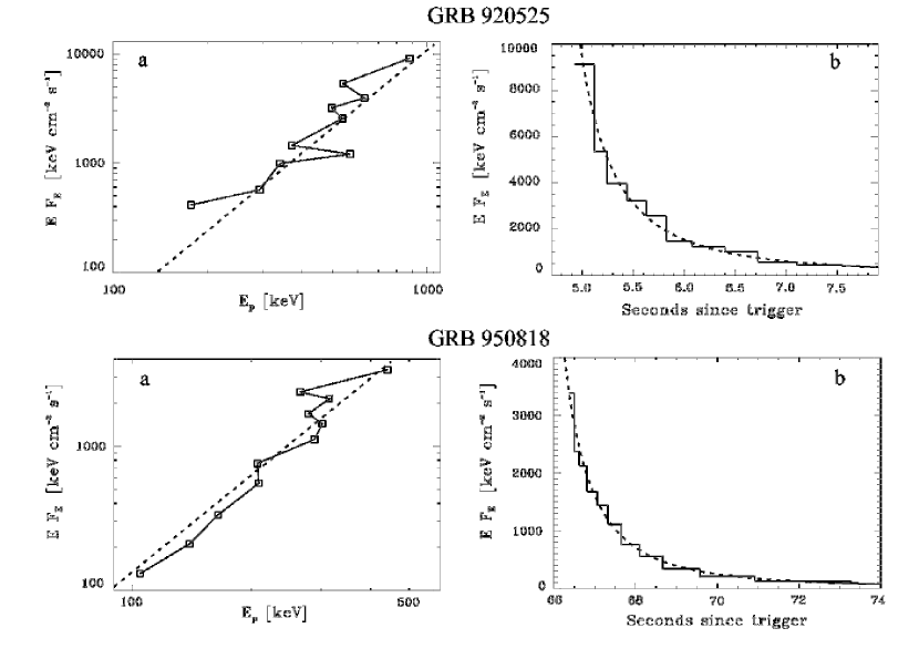
Figure 1: Examples of GRBs (squares and histograms) which follow the relations in equation (1) and (2) (dashed lines). (a) the HIC relations and (b) the pulse shapes for the decay phases of GRB 920525 (trigger 1625) with $\eta=2.4\pm 0.5$ and $d=2.0\pm 0.4$ and of GRB 950818 (trigger 3765) with $\eta=2.2\pm 0.3$ and $d=2.1\pm 0.4$.

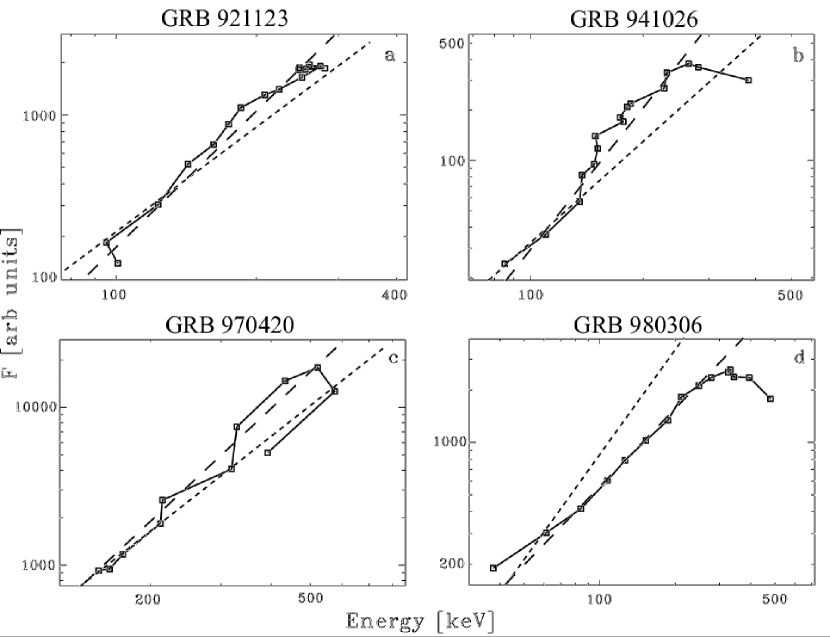
Figure 2: Hardness-intensity correlations (HICs) for four BATSE triggers with $\eta$ indexes deviating significantly from $\eta=2.0$. (a) GRB 921123 (trigger 2067) $\eta=2.60\pm 0.15$ (b) GRB 941026 (trigger 3257) $\eta=2.80\pm 0.20$ (c) GRB 970420 (trigger 6198) $\eta=2.38\pm 0.15$ (d) GRB 980306 (trigger 6630) $\eta=1.49\pm 0.04$. (see BR01 for details). The long-dashed lines show these power-law fits to the pulse decay-phase HICs. Note that the rise-phase HIC is included in the figures. The short-dashed lines show the $\eta=2$ power-law showing that the later phases of the pulse in (a,b,c) obey this relation (see discussion in §5).

2.2 Pulse Decay Shape

Investigations of the light curve (over the whole, observed spectral range) during pulse decay phases by Ryde & Svensson (2000) have shown that the observed photon flux, $F(E)/E$ or $F(\nu)/\nu$, can often be described by a reciprocal function in time. Ryde, Kocevski & Liang (2002) derive the corresponding decay shape for the bolometric energy flux ($F_{\rm bol}$), which in general can be described by

$$F_{\rm bol}(t)=F_{\rm bol,0}\left(1+\frac{t}{\tau}\right)^{-d}.$$ (2)

There is, however, an ambiguity in fitting such a light curve to the data. The values of the power-law index $d$ and the time constant $\tau$ are coupled and, consequently are often not well constrained by the fitting. Furthermore, a subjective judgement must be made in choosing the transition moment between the rise and the decay phases. As a result the pulse shape fitting does not provide as clear a signal as the HIC relation. This ambiguity is illustrated by F. Ryde, D. Kocevski, et al. (in preparation), who revisit the BR01 sample and analyze the deconvolved light curves and fit the light curves with equation (2). The parameters are indeed unconstrained in approximately half of the cases. Two of the constrained cases are shown in Figure 1b. Kocevski & Liang (2001) and Ryde, Kocevski & Liang (2002) introduce an approach to overcome this ambiguity by defining various analytical shapes for the whole pulse that include the rise phase (whenever present) and asymptotically approaches equation (2) in the decay phase. Kocevski & Liang (2001) studied a sample of 22 pulses with good rise phases and found $d=2.2\pm 0.7$.

A corollary of the above two relations is that $E_{\rm p}$ also decays following the above form with a different exponent.

$$E_{\rm p}(t)=E_{\rm 0}\left(1+\frac{t}{\tau}\right)^{-d/\eta}.$$ (3)

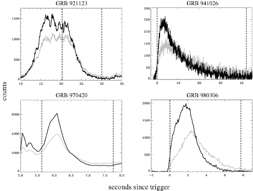
Figure 3: Background-subtracted, count light-curves (64 ms resolution) for the four triggers in Figure 2. For each trigger the light curve for two different spectral bands are shown; in gray, BATSE channel 2 (55 - 110 keV) and, in black, BATSE channel 3 (110 - 325 keV). The time interval used for the HICs in Figure 2 are indicated by the dashed lines.

2.3 Change of Pulse Shape with Spectral Band

In this paper we will mainly focus on the observed behavior of the spectral evolution as described by the HIC and the shape of the pulse decay phase. There are, however, several other approaches that can be used to present the observed evolution. One way is to study the change in pulse shape and width over different spectral bands and the time lag between these bands (see, e.g., Norris, Marani, & Bonnell (2000)). To illustrate this we present in Figure 3 the light curves of the four cases shown in Figure 2. For each case we show the light curve in two energy bands. For more detailed discussion on this approach we refer to F.Ryde, D.Kocevski, et al. (in preparation).

3 TIME SCALES

There are many time scales in a GRB. In this paper we are interested in the effects of the curvature of the emission front and the time scale it introduces in the pulse shape. In order to find the importance of this effect its time scale should be compared to the radiative cooling time and the dynamic time for the crossing (or merger) of two shells.

Estimation of the cooling time, which we assume is comparable or longer than the acceleration time, requires a knowledge of the emission and energy loss processes of electrons. The details of the acceleration mechanism are not known, but it is generally assumed that the dissipation of the kinetic energy of the fireball gives rise to a power law distribution of electrons. The minimum random Lorentz factor of the electrons is proportional to the relative Lorentz factor; $\gamma_{\rm{e}}=\xi_{\rm{e}}(m_{\rm{p}}/m_{\rm{e}})(\Gamma_{\rm{rel}}-1)$, where $m_{\rm{e}}$ and $m_{\rm{p}}$ are the electron and the proton masses, respectively, and $\Gamma_{\rm{rel}}=\Gamma_{\rm{1}}\Gamma_{\rm{2}}(1-\beta_{1}\beta_{2})\sim\Gamma_{\rm{1}}/(2\Gamma_{\rm{2}})$, which is of the order of $10$ or lower, is the relative Lorentz factor between the two interacting shells ($\Gamma_{\rm{1}}>\Gamma_{\rm{2}}$). $\xi_{\rm{e}}$, and $\xi_{\rm{B}}$ introduced below, are the fractions of the post-shock, random energy density that resides in the electrons and the magnetic field. The magnetic field strength is given by $B=(32\pi\xi_{\rm{B}}n^{\prime}m_{\rm{p}}c^{2}\Gamma_{\rm{rel}})^{1/2}\sim 2\times 10^{4}$ Gauss, where we assume equipartition and a comoving electron density $n^{\prime}=L_{\rm{kin}}/4\pi R^{2}\Gamma^{2}m_{\rm{p}}c^{3}\sim 2\times 10^{10}$ cm^-3, for an assumed kinetic luminosity of $L_{\rm{kin}}\sim 10^{53}$ erg/s, distance $R$ of $10^{15}$ cm, and a shock compression ratio of 4.

In the rest frame of the progenitor the cooling time scale for a particle of comoving energy $E^{\prime}$ and loss rate $\dot{E^{\prime}}$ is dilated to $\tau_{\rm loss}=\Gamma E^{\prime}/\dot{E^{\prime}}$. As the emitting material is moving towards the observer the rest-frame time scales will be compressed by a factor $(1-\beta)^{-1}\sim 2\Gamma^{2}$ in the observer frame (see below). If the pulse shape is determined solely by the radiative cooling process then, for the above parameters and assumptions, the observed decay time scale of the pulse will be

$$\tau_{\rm cool} = \frac{E}{2\Gamma|\dot{E_{\rm s}}+{\dot{E_{\rm{IC}}}}|}=\frac{3\pi m_{\rm{e}}c}{\Gamma\sigma_{\rm{T}}\gamma_{\rm{e}}B^{2}(1+U_{\rm{rad}}/U_{\rm{B}})}$$ (4)

$$\sim 6\times 10^{-5}\,{\rm s}(\Gamma_{\rm{rel}}-1)^{-2}\left(\frac{R}{10^{15}{\rm cm}}\right)^{2}\left(\frac{\Gamma}{100}\right)\left(\frac{L_{\rm kin}}{10^{53}}\right)^{-1}$$

Here subscripts s and IC refer to the cooling rates due to synchrotron and inverse Compton losses in radiation and magnetic field energy densities of $U_{\rm rad}$ and $U_{B}=B^{2}/(8\pi)$. This is a much shorter time scale compared to the dynamic and curvature times discussed below.

The curvature time scale arises from relativistic effects in a sphere expanding with a high bulk Lorentz factor $\Gamma$. Due to the curvature of the shell there will be a time delay between the photons emitted simultaneously in the comoving frame from different points on the surface. Figure 4 shows the geometry of the situation. Due to the relativistic aberration of light, isotropically emitted radiation in the comoving frame will be beamed into a cone with opening angle $\theta\sim\Gamma^{-1}$. Only photons emitted from the fireball surface within a narrow cone of opening angle $\sim\Gamma^{-1}$ around the LOS will be detectable by the observer. The typical time delay is thus $\tau_{\rm ang}=R[1-\cos(1/\Gamma)]/c$ which for large $\Gamma$ is approximately $R/(2\Gamma^{2})c$. This gives a lower bound for the observed duration of a pulse:

$$\tau_{\rm ang}=1.7{\rm s}\left(\frac{R}{10^{15}{\rm cm}}\right)\left(\frac{\Gamma}{10^{2}}\right)^{-2}.$$ (5)

The dynamic time scale for a single pulse is the actual crossing (or merger) time of one shell with another. Often the shell collision is assumed to be an inelastic collision and the merged shells expand as a single shell. The shell crossing time is $\tau_{\rm dyn}^{\prime}=\Delta^{\prime}/v^{\prime}_{\rm sh}$, where ${v^{\prime}_{\rm sh}}$ is the velocity of the shock in the comoving frame of the preshocked flow. The initial value, and the evolution with radius, of the shell width $\Delta^{\prime}$ are not well understood and depend, among other factors, on the structure and internal dynamics of the shell and on its interaction with the external medium. If the Lorentz factor is constant over the shell, or if the shell is confined by some mechanism, then the shell width will be independent of radius and time, $\Delta=\Delta_{0}$. But if there exists a differential flow with a faster leading and a slower trailing edge with velocities $\beta_{\rm r}$ and $\beta_{\rm s}$, and corresponding Lorentz factors $\Gamma_{\rm r}$ and $\Gamma_{\rm s}$, respectively, then

$$\Delta(R)=R(\beta_{\rm r}-\beta_{\rm s})=\frac{R}{2\Gamma_{\rm s}^{2}}\left[1-\left(\frac{\Gamma_{\rm s}}{\Gamma_{\rm r}}\right)^{2}\right]\sim\frac{R}{2\Gamma_{\rm s}^{2}},$$ (6)

where for the last relation we have assumed that $\Gamma_{\rm s}\ll\Gamma_{\rm r}$. In the comoving frame $\Delta^{\prime}(R)=R/(2\Gamma_{\rm s})$. This relation will be applicable at radii $R>R_{\rm b}=\Delta_{0}\Gamma^{2}$, where the spread will exceed the initial width. The shell crossing time is then $\tau_{\rm dyn}^{\prime}=\Delta^{\prime}/v^{\prime}_{\rm sh}=R/(\Gamma_{\rm s}v^{\prime}_{\rm sh})$. In the observer frame these times will be time-dilated and affected by the motion of the fireball towards the observer:

$$\tau_{\rm dyn}=\frac{\tau_{\rm dyn}^{\prime}}{2\Gamma}=\frac{R}{4\Gamma_{\rm s}\Gamma v_{\rm sh}^{\prime}}=1\,{\rm s}\,\beta^{\prime-1}_{\rm sh}\left(\frac{R}{10^{15}}\right)\left(\frac{\Gamma}{100}\right)^{-2}\left(\frac{\Gamma}{\Gamma_{\rm s}}\right).$$ (7)

For the assumptions described above the dynamic time scale is somewhat shorter than (and has a similar dependence on $R$ and $\Gamma$) as the curvature time scale; $\tau_{\rm ang}\sim 2(\Gamma_{\rm s}/\Gamma)\tau_{\rm dyn}$. However, at smaller values of $R<R_{b}$, where the spreading is negligible, the dynamic time scale may exceed the angular one by $R_{b}/R$. Since, in general, the pulse width is proportional to $R$, the latter situation is more likely to arise in shorter pulses.

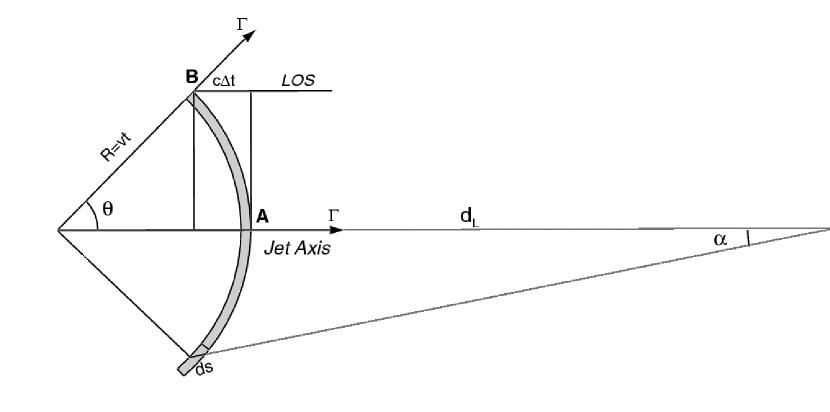
Figure 4: Geometrical sketch of the visible part of the fireball. Due to the relativistic aberration of light, the main part of the radiation comes out within a small cone with half opening angle $\theta\sim\Gamma^{-1}$. Note that the line of sight (or LOS) and the jet axis do not need to be parallel. The photons from A are boosted by $2\Gamma$ but those from B, which are delayed by $\Delta t=R/c(1-\mu)$, are boosted by $[\Gamma(1-\beta\mu)]^{-1}$, where $\mu=\cos\theta$.

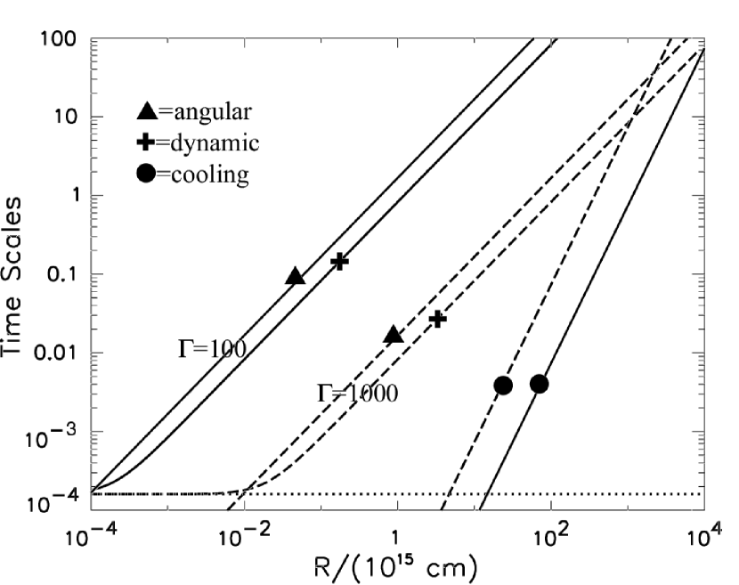
Figure 5: The radial dependence of the various time scales. The solid lines are for a bulk Lorentz factor of $\Gamma=100$, while the dashed lines are for $\Gamma=1000$. For the cooling time we have used eq. (4) with $\Gamma_{\rm rel}=10$ and a kinetic luminosity $L_{\rm kin}=10^{53}$ erg/s, and the angular time is given by equation (5). For the dynamic time we have used equation (7) with $\Gamma_{s}\sim\Gamma=100$ and $\beta^{\prime}_{\rm sh}=1$. If the shell width is constant, $\Delta=\Delta_{0}$, then there will be a minimum dynamic time scale at all $R$ and be represented by a horizontal line in the figure; Assuming $\Delta_{0}=10^{9}$ cm, $\tau_{\rm dyn}=1.6\times 10^{-4}$ s ${\beta^{\prime}_{\rm sh}}^{-1}(\Gamma/100)^{-1}(\Delta_{0}/10^{9}$ cm).

Figure 5 shows the radial dependence of the three time scales, $\tau_{\rm cool}$(eq. 4), $\tau_{\rm ang}$(eq. 5), $\tau_{\rm dyn}$ (eq. 7), for two values of the bulk Lorentz factor $\Gamma$, for $\Gamma\sim\Gamma_{\rm s}$, and for $R_{b}=10^{11}$ cm. From this we conclude that in situations with sufficiently narrow shells, the curvature effects can indeed be the determining factor for the pulse decay time scale. Correspondingly, if these effects are shown to be important in the observed pulses, this could set a constraint on the thickness (value of $\Gamma_{\rm s}/\Gamma_{\rm r}$) and the spreading of the shell (values of $R_{b}$ and $\Gamma_{\rm s}$) and/or on the distance $R$ where the radiation is emitted. The curvature effect becomes important if $\tau_{\rm ang}>\tau_{\rm dyn}$. This happens for shell widths $\Delta^{\prime}\lower 2.15277pt\hbox{$\;\buildrel<\over{\sim}\;$}\beta^{\prime}_{\rm sh}R/\Gamma$. Even in the case with linearly increasing shell-width the angular effect will be noticeable and can be totally dominating if the shell is narrower (e.g. if the shell-width stays constant). Spada, Panaitescu, & Mészáros (2000) simulated internal shocks and found that with a linear shell broadening, as above, the angular spreading and the shock crossing times are comparable.

In the following we consider a scenario where the rise phase of a pulse corresponds to the merging phase or the dynamic evolution, while the decay phase arises as a purely kinematical effect due to the curvature of the relativistically expanding shell. The acceleration and radiative cooling times are assumed to be much shorter than or at most comparable to the dynamic time.

4 RELATIVISTIC KINEMATICS

The radiation from a relativistically expanding plasma sphere (fireball) will have a unique signature in the observer frame. We start by studying the radiation observed from an infinitely thin spherical shell and thereafter generalize the problem to broader shells. We assume that the visible part of the fireball is spherically symmetric and homogeneous, i.e., only one parameter is enough to characterize the properties of a patch of emission. This type of problem has previously been discussed by, among others, Fenimore et al. (1996), Granot et al. (1999) and Eriksen & Grøn (2000).

4.1 Lorentz Boosting and Spectrum Evolution

The Lorentz boosting factor for transformation from the comoving frame to the observer frame of photons emitted into the LOS from different locations on the surface, defined by the angle $\theta\equiv\arccos\mu$ shown in Figure 4 is

$${\cal D}(\Gamma,\mu)=\frac{1}{\Gamma(1-\beta\mu)}=\Gamma(1+\beta\mu^{\prime}).$$ (8)

For small angles this reduces to ${\cal D}(\Gamma)=2\Gamma$, which is the boost factor used in discussing GRB emission, when the angular dependence is not considered important (e.g. flat shell perpendicular to LOS).

If we set $\theta=0$ at the point where the flow velocity is parallel to LOS (point A in Fig. 4), then the difference in light travel time $\Delta t$ between photons emitted along the LOS from this point and a point at an angle $\theta$ (point B in Fig. 4) is $\Delta t=R_{0}(1-\mu)/c$ , which gives $\mu=1-c\Delta t/R_{0}$. Inserting this into equation (8) we find

$${\cal D}(\Gamma,\Delta t)=\frac{1}{\Gamma(1-\beta+\beta c\Delta t/R_{0})}.$$ (9)

For highly relativistic outflows $\beta=1-(2\Gamma^{2})^{-1}$, and

$${\cal D}(\Gamma,\Delta t)=2\Gamma(1+\Delta t/\tau_{\rm ang})^{-1},\,\,\,\tau_{\rm ang}\equiv R_{0}/(2\Gamma^{2}c).$$ (10)

An obvious outcome of this is that if the emitted spectra from different parts of the shell are identical, then the observed spectrum will be boosted (gradually redshifted) in time by a factor ${\cal D}$ as different parts of the surface come into view. In particular the peak energy will evolve as

$$E_{\rm p}(t)=E^{\prime}_{\rm p}{\cal D}=\frac{E_{\rm 0}}{(1+t/\tau_{\rm ang})},$$ (11)

where $E^{\prime}_{\rm p}$ is the peak energy in the comoving frame (which is the same at all angles), $E_{\rm 0}=E^{\prime}_{\rm p}2\Gamma$, and we have set $\Delta t=t$, which assumes that $t=0$ for radiation observed from point A in Figure 4.

4.2 Energy Flux and the Light Curve

We want to determine the pulse shape, in bolometric energy flux, assuming it to be entirely caused by the above angular dependence of the Lorentz boost variation. This means we are considering a situation where $\tau_{\rm dyn}$ and $\tau_{\rm cool}\ll\tau_{\rm ang}$. We, therefore, initially assume a simple isotropic volume emissivity.

$$j^{\prime}=\Sigma^{\prime}\,\delta(t^{\prime}-t_{0})\,\delta(R^{\prime}-R_{0}),$$ (12)

where $\Sigma^{\prime}$ is the total, rest frame, energy surface-brightness. More complex temporal and spatial distributions will be discussed in the next section. [We follow the formalism outlined in Granot et al. (1999) and refer to Figure 4.] We also introduce the following variables: the luminosity distance $d_{\rm L}$, the viewing angle $\alpha=\sin\theta R/d_{\rm L}=(1-\mu^{2})^{1/2}R/d_{\rm L}$ so that $\alpha d\alpha=(R/d_{\rm L})^{2}\mu\,d\mu$. Using the Lorentz invariance of $j/\nu^{3}$ (Rybicki & Lightman, 1979) we can write the observed intensity (neglecting cosmological redshift factors) as

$$I=\int jds=\int j^{\prime}{\cal{D}}^{3}dR/\mu$$ (13)

and the observed bolometric energy flux as

$$F_{\rm bol}=\int\mu Id\Omega=\int\int\int j^{\prime}{\cal{D}}^{3}dR\sin\alpha d\alpha d\Phi$$ (14)

where $ds$ is the element of length through the shell along the LOS, $\Phi$ is the azimuthal angle and $d\Omega$ is the solid angle of the source as seen by the observer. Assuming azimuthal symmetry around the jet axis ($\int d\Phi=2\pi$) we get

$$F_{\rm bol}(t)=\frac{1}{2d_{\rm L}^{2}}\int_{0}^{\infty}R^{2}dR\int_{-1}^{1}\;\mu\,d\mu\,{\cal{D}}^{3}(4\pi j^{\prime}).$$ (15)

Using the transformations $|dR/dR^{\prime}|=\Gamma^{-1}$, $|dt_{\rm obs}/dt^{\prime}|={\cal D}^{-1}$, and that $dt=(R/c)\,d\mu$ we get $\delta(t^{\prime}-t_{0})\delta(R^{\prime}-R_{0})=c\,(R\Gamma{\cal{D}})^{-1}\,\delta(\mu-\mu_{0})\delta(R-R_{0})$. The observed flux then can be written as

$$F_{\rm bol}(t)=F_{0}\mu{\cal{D}}^{2}(\mu)/\Gamma^{2},\,\,{\rm with}\,\,F_{0}\equiv{2\pi\Sigma^{\prime}R_{0}c\Gamma}/{d_{\rm L}^{2}},$$ (16)

where the time dependence arises from the relation $\mu=1-ct/R_{0}$. For a highly relativistic outflow (where $\theta_{\rm max}\sim 1/\Gamma$) the projection factor $\mu=\cos\theta$ in equation (16) is less than $1-(2\Gamma^{2})^{-1}$ and can be ignored so that $F_{\rm bol}(t)=F_{0}{\cal D}^{2}(\mu)/\Gamma^{2}$. Note that the above result is independent of whether the outflow is completely spherical or confined or collimated into a jet of opening angle $\theta_{\rm jet}$, as long as $\theta_{\rm jet}>\Gamma^{-1}$.

Now with the help of equation (9), and identifying the time delay $\Delta t$ with the time $t$ as above, we get

$$F_{\rm bol}(t)=F_{0}/(1+t/\tau_{\rm ang})^{2}.$$ (17)

This surprisingly is very similar to the observed behavior of the small sample of well-isolated pulses described in §2.

4.3 Flux-Spectrum Correlation; HIC

In the $\delta$-function approximation, and if the bulk Lorentz factor and if the rest frame flux and spectrum are independent of position along the surface of the shell (i.e. we have a homogeneous source), then equations (11 and 17) will describe the spectral and flux evolutions adequately. This can be translated into a measurable hardness-intensity correlation if we represent the hardness by the value of $E_{\rm p}$. The observed HIC (eq. [1]) follows directly: $F\propto E_{\rm p}^{\eta}$, with a power-law index of $\eta=2$, which is equal to the observed average value found in BR01.

Another way to look at this relation is through the time evolution of the energy fluence defined as ${\cal{E}}(t)\equiv\int_{0}^{t}F(\tilde{t})d\tilde{t}$. Using equation (17) it can easily be shown that

$${\cal{E}}(t)={F_{0}\tau}\left[1-(1+t/\tau_{\rm ang})^{-1}\right],$$ (18)

which when inserted into equation (11) gives

$$E_{\rm p}=E_{\rm p,0}-\frac{{\cal E}E_{\rm p,0}}{F_{\rm 0}\tau_{\rm ang}},$$ (19)

which is the so-called hardness-fluence correlation (HFC). The inverse of its proportionality constant is usually denoted by $\Phi_{\rm 0}$ (Liang & Kargatis, 1996; Ryde & Svensson, 2000), so in this description $\Phi_{\rm 0}=F_{\rm 0}\tau_{\rm ang}/E_{\rm p,0}$.

5 FINITE DYNAMICAL TIME

The above analysis assumes a very short dynamic, as well as cooling, time scales relative to the curvature time delay. This allows the delta function time profile approximation used in §4.2. However, as mentioned above and shown in Figure 5, the dynamic time $\tau_{\rm dyn}$, which in our model defines the rise time of the pulse, could be comparable to (and in short pulses it may exceed) the curvature time scale. Therefore we must examine the effects of finite $\tau_{\rm dyn}$.

5.1 Bolometric Light Curves

For a shell shining continuously for a finite period of time the resulting pulse profile will be a convolution of the comoving frame emissivity time profile, say $j^{\prime}(t^{\prime})=\Sigma^{\prime}f(t^{\prime})$, with $\int f(t^{\prime})dt^{\prime}=1$, and the profile due to the curvature effect (eq. [11]) obtained from an impulsive intrinsic emission profile, $f=\delta(t^{\prime}-t^{\prime}_{0})$. The emissivity profile, when transformed to the observer frame, retains its form but its characteristic time scale is scaled by the boost factor; $\tau_{\rm dyn}^{\prime}=\tau_{\rm dyn}{\cal D}$. The resultant pulse profile then becomes

$$F_{\rm bol}(t)=F_{\rm 0}\int_{t}^{+\infty}f(t-x)dx/(1+x/\tau_{\rm ang})^{2}$$ (20)

Figure 6 illustrates the effects of the finite emission time scale for the intrinsic pulses. In the three top panels the intrinsic pulses were modeled as decaying exponentials with time scale $\tau_{\rm dyn}$. The shape of the convolved light curve is determined by the ratio of the intrinsic emission time scale $\tau_{\rm ang}$ to that of the curvature $\tau_{\rm dyn};{\cal R}=\tau_{\rm ang}/\tau_{\rm dyn}$. In general the convolved pulse will resemble a FRED (fast rise and exponential decay). Different ratios of the time scales give rise to pulse shapes that encompass the actual observed pulse shapes by BATSE. For long duration pulses the convolved light curves will asymptotically reach the $d=2$ form of equation (2) and manifest the curvature effect. But for short and weak bursts this stage may not be observable and one sees a pulse shape determined by the dynamics of the shell crossing. The general behavior is well illustrated by these three cases. However, other intrinsic pulse shapes do give rise to some variations. For instance, including an intrinsic rise phase will broaden the rise phase of the convolved light curve, as illustrated by the bottom panels in which the intrinsic pulses were modeled by symmetric Gaussians of half width $\tau_{\rm dyn}$.

It should be emphasized again that in the discussion above, and in equation (20) in particular, we are dealing with the bolometric flux, using the approach introduced in BR01, who represent this flux by $EF_{\rm E}$ evaluated at $E_{\rm p}$. In general, however, for a finite observation band there will be a time dependence term beyond what is shown in equation (20). If, over a finite dynamic time, the spectrum evolves, i.e. the $E_{\rm p}$ changes, the flux contribution within the observed band, and consequently the bolometric correction will change (the amount of changes depending on the values and/or evolution of indexes $\alpha$ and $\beta$). This will affect the above light curve as well as the HIC relation described next. In an approach different from BR01, to account for this issue, Fenimore & Sumner (1997); Fenimore et al. (1996) instead assumed a photon number spectrum described by a single power law with index equal to the averaged value $(\alpha+\beta)/2$, and calculated the observed photon flux over a certain band pass which thus changes in the observer frame with time. The relation between the photon flux and the peak energy found by this method was studied by Soderberg & Fenimore (2001) who concluded that a long cooling time was necessary to explain the data.

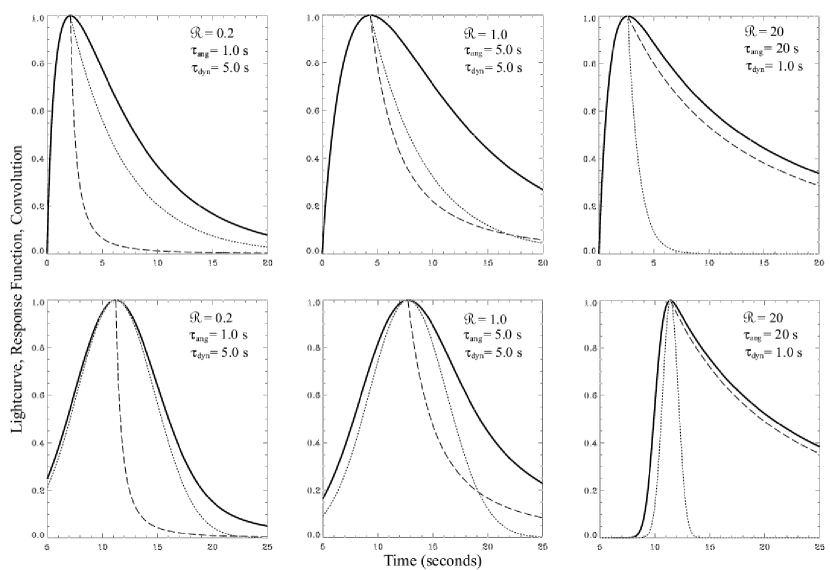
Figure 6: Light curve behaviors in the observer frame, with varying parameter combinations of the exponential decay constant $\tau_{\rm dyn}$ and the angular time scale $\tau_{\rm ang}$. The dotted, dashed, and solid lines represent the comoving light curve, the relativistic angular spread function and the convolved light curve. Top panels for a one-sided (zero rise time) exponential intrinsic light curve $f\propto\exp(-t/\tau_{\rm dyn}),\,\,t>0$. Note that the convolved light curve has a finite rise time. The lower panels for a symmetric Gaussian intrinsic light curve, $f\propto\exp(-t/\tau_{\rm dyn})^{2}$, for $-\infty<t<\infty$. The comoving light curves and the angular spread functions are normalized to have the $t=0$ at the peak of the observed (convolved) pulse.

5.2 Spectra and HICs

The effects of a finite emission pulse on the spectral behavior are more complicated. This is because the instantaneous spectra, as seen by the observer, will be a superposition of spectra from several annuli emitted at different times having different $\mu=\cos\theta$, boost factor ${\cal D}(\mu)$, and perhaps different spectral hardness (say different $E_{\rm p}$) and shape (different indexes $\alpha$ and $\beta$). Let us assume that the intrinsic spectrum, as observed in the rest frame, can be described by two spectral indexes $\alpha$ and $\beta$ and a break or peak energy $E_{\rm p}$, say a Band et al. (1993) function, ${\cal B}_{\alpha,\beta}(E/E_{\rm p})$, with $\int_{0}^{\infty}{\cal B}\,dE=1$. To simplify matters, we further assume that $\alpha$ and $\beta$ are constant so that the only spectral variation is due to changes in $E_{\rm p}$. We will represent the evolution of $E_{\rm p}$ by an intrinsic HIC relation with index $\eta_{\rm int}$, $F\propto{E_{\rm p}}^{\eta_{\rm int}}$, which means that $E_{\rm p}(t)=E_{\rm p,0}[f(t)]^{(-1/\eta_{\rm int})}$. The observed flux spectrum at any time can thus be written as

$$F(E,t)=F_{0}\int_{t}^{\infty}\frac{f(t-x)}{(1+x/\tau_{\rm ang})^{2}}{\cal B}_{\alpha,\beta}\left(\frac{E}{E_{\rm p}(t,x)}\right)\,dx,\,\,\,$$ (21)

with

$$E_{\rm p}(t,x)=E_{\rm p,0}(1+x/\tau_{\rm ang})^{-1}[f(t-x)]^{(-1/\eta_{\rm int})}$$ (22)

When integrated over all energy, equation (21) reduces to equation (20). Note that the resultant spectra or light curves depend primarily on the ratio of the time scales, ${\cal R}=\tau_{\rm ang}/\tau_{\rm dyn}$ defined above. Secondary factors are the intrinsic pulse shape and HIC relation.

Before showing the resultant HIC for different cases we first discuss the details of the formation of the observed spectra. For the purpose of illustration we assume $\alpha=-2/3,\beta=-2.5$ and three different values for the index $\eta_{\rm int}$. To simplify the description of how the contributing spectra make up the integrated spectrum we start with the case of an intrinsic light curve with an abrupt rise phase and a simple exponential decay phase: $f(t)={\tau_{\rm dyn}}^{-1}\exp(-t/\tau_{\rm dyn}),\,\,{\rm for}\,\,t>0$. The effects of intrinsic pulses with a finite rise phase are discussed below. Note that an intrinsic pulse with only a decay phase will still produce a rise phase for the observer due to the convolution described above. For such an intrinsic pulse, the upper limits of the integrals in eq. (20) and (21) are zero, so that at any given time $t$ the observer receives signals from annuli extending from $\theta=0$ to $\theta=\theta_{\rm max}(t)$ or $1<\mu<\mu_{\rm min}=(1-\beta ct/R_{0})$. Different angles $\theta$ sample different stages of the intrinsic spectral evolution due to the angular spreading of the signal, with the spectrum from $\theta_{\rm max}(t)$ being that emitted at the beginning of the pulse and the spectrum from $\theta=0$ reflecting that of a later time in the pulse. Equation (21) gives the convolved spectrum as a superposition of different spectra from different angles or different times.

In the absence of the curvature effect (i.e. for a flat shell, $R_{0}\rightarrow\infty$, or $\tau_{\rm ang}$ and ${\cal R}\rightarrow 0$) one would observe the intrinsic HIC relation. It follows then that for a finite $\tau_{\rm ang}$ but for ${\cal R}\ll 1$, this is the HIC relation that will be observed except for a short time $t\sim\tau_{\rm ang}$ at the beginning (and the rising phase) of the observed pulse. In the opposite limit of ${\cal R}\gg 1$, the delta function approximation result with the HIC relation $F_{\rm bol}\propto E_{\rm p}^{2}$ is obtained, again except for a short time $t\sim\tau_{\rm dyn}$ at the beginning (and the rising phase) of the observed pulse.

For ${\cal R}$ of the order of unity, one expects a combination of these two behaviors. For the assumed exponential intrinsic light curve, which (for ${\cal{R}}\sim 1$) dies more quickly than the light curve shape induced by the curvature effect, we expect an initial phase when the HIC obeys the intrinsic form ($\eta\sim\eta_{\rm int}$) followed eventually by the relation expected from the curvature effect ($\eta=2$). This transition can be seen in Figure 7 for the three cases with ${\cal R}=0.5,1$ and 2, from the top to the bottom panels. In each panel we show total spectra for four different observed times $t$ (solid curves). The circles show the peak flux and the photon energy at the peak (i.e. the observed $E_{\rm p}$) for these four and several more total spectra. This is what the observed HIC will look like. The light dotted lines show the assumed intrinsic, $\eta_{\rm int}=1$, and the curvature-induced, $\eta=2$, HIC relations. Each one of the total spectra is a sum of the spectra from different angles $0<\theta<\theta_{\rm max}(t)$ with different $E_{\rm p}$’s having suffered different boosts. The peak flux and the peak energy of spectra from several angles are shown by the crosses for each of the four observer times. The crosses furthest to the left represent the $\theta=0$ spectrum which is identical to the intrinsic spectrum (of course boosted by $2\Gamma^{2}$) and, therefore, lies on the dotted line with slope $\eta_{\rm int}=1$. As we move to the right we see spectra from successively larger $\theta$s (with varying boosts) till the crosses furthest to the right which are for $\theta_{\rm max}$, i.e., the radiation emitted at $t=0$, with the flux and $E_{\rm p}$ boosted according the relations described in the previous section, and lies on the dotted line with the slope $\eta=2$.

For the lower panel, ${\cal R}=2$, the most intense radiation comes from $\theta_{\rm max}$. Consequently, the total spectra obey the large ${\cal R}$, or delta function, HIC relation ($\eta=2$), except for a relatively short but noticeable initial phase. For smaller ${\cal R}$ this initial phase increases in length. As evident from the relative position of the crosses in the panel for ${\cal R}=0.5$, for the first two times shown, the emission is dominated by the radiation from $\theta=0$ and we obtain a well defined HIC with $\eta=\eta_{\rm int}=1$. But by the time corresponding to the fourth total spectrum the emission from $\theta_{\rm max}$ dominates and the HIC reverts to the $\eta=2$ case. The location of the crosses and the final HIC relation for the ${\cal R}=1$ case is intermediate between the above two cases.

In order to further demonstrate the relative effects of the intrinsic and curvature-induced HIC relations, in Figure 8 we show two cases with ${\cal R}=1$ but with intrinsic power law indexes, $\eta_{\rm int}=0.5$ and $\eta_{\rm int}=\infty$. The latter corresponds to a constant $E_{\rm p}$ independent of the flux. In Figure 9 we show only the resultant HIC relation for five different values of ${\cal R}$ for the above three intrinsic HIC indexes $\eta_{\rm int}=.5,1$ and $\infty$.

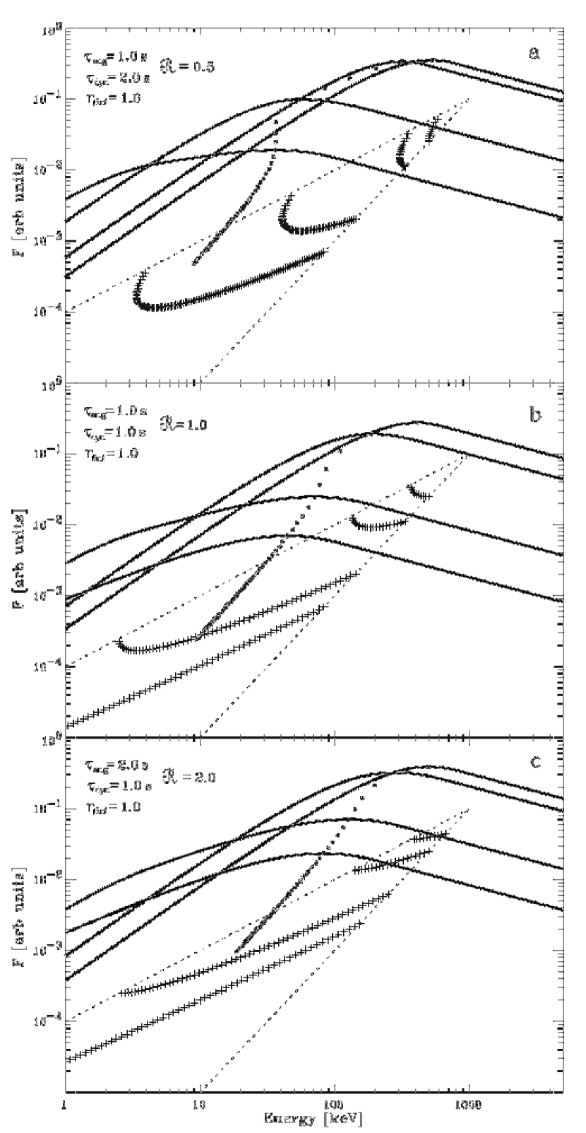
Figure 7: Observer frame spectra (solid lines) at four different times (1, 2, 6 and 11 s; where the first light is detected at $t=0$ s). These spectra are found by integrating the intrinsic spectra over $\theta$. The positions in the $F-E_{\rm p}$ plane of the peaks of some of these contributing spectra are indicated by large crosses. The upper and lower dashed lines represent, respectively the locii at $\theta=0$ which follow the intrinsic evolution of the HIC relation (here assumed to be a power law with intrinsic HIC index, $\eta_{\rm int}=1.0$), and at $\theta=\theta_{\rm max}$ obeying the HIC relation expected from the curvature effect (with a power-law with index $\eta=2$). The circles show the HIC relation of the convolved spectra in time steps of 1 s, up to $t=60$ s: (a) ${\cal R}=0.5$ (b) ${\cal R}=1.0$ (c) ${\cal R}=2.0$.

Figure 8: Same as Fig. 7 for ${\cal R}=1.0$, but two different intrinsic HIC relations (a) $\eta_{int}=0.5$ and (b) $\eta_{int}=\infty$ corresponding to a constant $E_{\rm p}^{\prime}(t)$. The softening of the observer frame low-energy spectra is clearly seen in (a) while (b) demonstrates that for steep intrinsic HICs ($\eta_{\rm int}>2$), the slope of the observed HIC will mainly be 2, independent of the intrinsic slope (see also Fig. 9a).

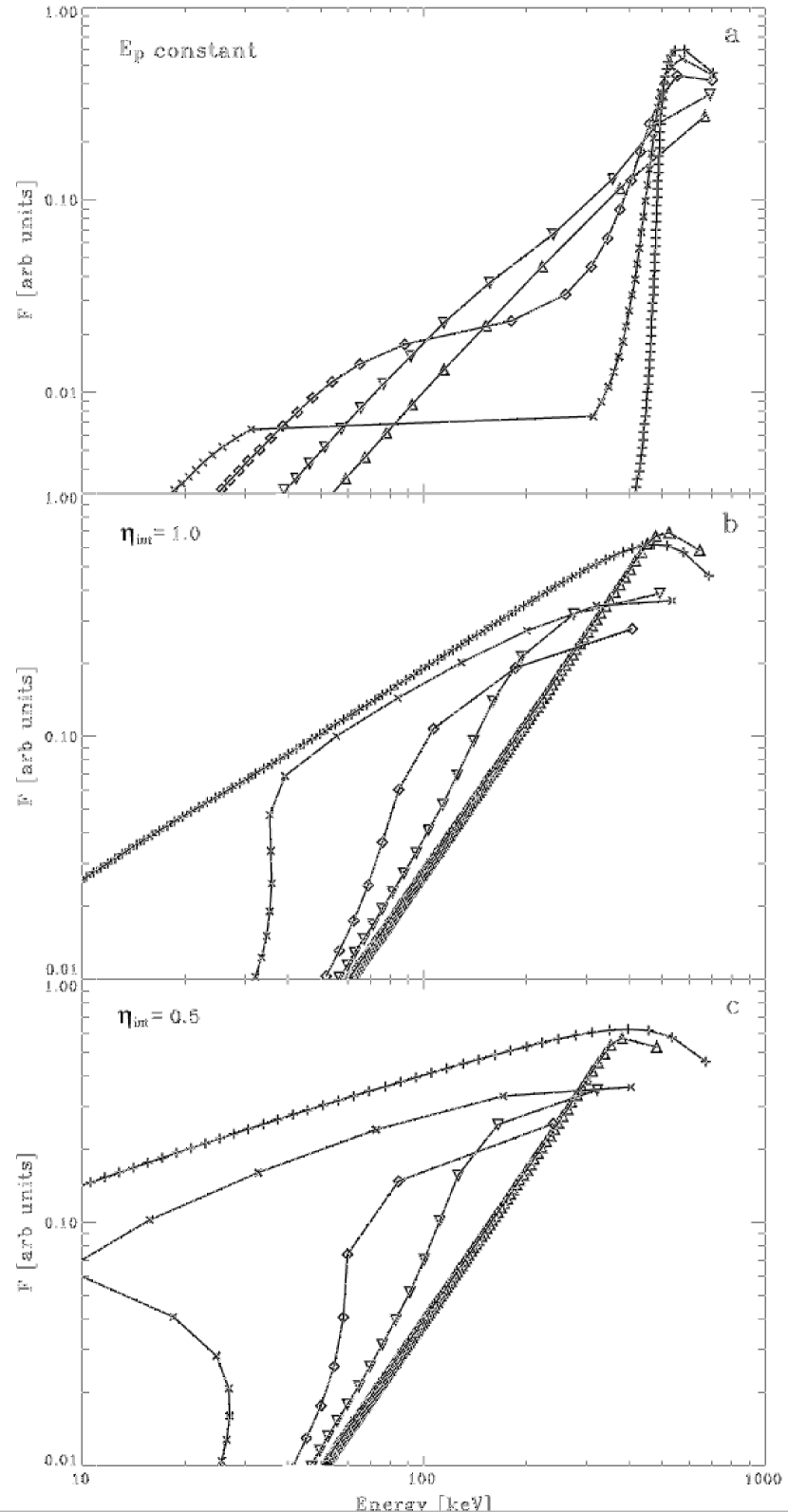
Figure 9: Observer frame HIC relations, for different values of ${\cal{R}}$, produced by three different intrinsic HIC relations: (a) $\eta_{int}=\infty$ (b) $\eta_{int}=1$ (c) $\eta_{int}=0.5$. In panel (a) the time steps are 2 s and ${\cal R}=0.05$ (crosses), 0.1 (x-es), 0.2 (diamonds), 0.5 (inverted triangles), 1.0 (triangles), while in panel (b) and (c) the time steps are 1 s and ${\cal R}=0.05$ (crosses), 0.5 (x-es), 1.0 (diamonds), 2.0 (inverted triangles), 20 (triangles). Note the presence of various concave HICs which can explain observed bursts with index $>2$, when fitted with a single power law.

Several conclusions can be drawn from these figures. The first is that the observed evolution of $E_{\rm p}$ may have nothing to do with the intrinsic evolution of the emission process, so that care is necessary in the interpretation of the observed spectral parameters. This is most clearly evident in Figure 8b where a non-evolving spectrum appears to have a HIC index of $\eta=2$. It is also clear (from all of the figures) that this most commonly observed HIC index does not require a very large value of the ratio ${\cal{R}}$. It is established after a few dynamic times for ${\cal{R}}=1$ and is omnipresent for ${\cal{R}}>2$, independent of the value of $\eta_{\rm int}$. On the other hand, the intrinsic HIC is essentially what is observed (at least when the flux is high, say down to $1$ % of peak flux) for ${\cal{R}}<0.5$.

It is clear that if there is some dispersion in the intrinsic power-law index, $\eta_{\rm int}$, for instance, if it has a broad, uniform distribution between 0 and $\infty$, then the observed distribution will be peaked around $\eta=2$. If the intrinsic source of radiation is synchrotron emission the preferred value of $\eta_{\rm int}$ will lie between $1$ and $2$ (Lloyd & Petrosian, 2002) and the observed distribution is expected to be even more peaked around 2. However, a variety of other possible values of this index and deviations from a simple power law will also be present. This is true especially for values of ${\cal R}\sim 1$. In addition, limitations imposed by the instrumentation make it possible to follow only a portion of the HIC. This is because the signal-to-noise of the observations limits the dynamic range of the observable flux and the finite band width of the instrument introduces bias against spectra with $E_{\rm p}$ outside the band. As is evident from Figures 7, 8, 9 some of the curves do not follow a perfect power law but are concave, which is even more pronounced for smaller $\eta_{\rm int}$. Thus a simple power law fit to these curves, excluding the few early phase points which may appear as part of the rise phase of the pulse, will yield a steep HIC with $\eta>2$. In fact inspection of the pulses with large measured $\eta$-values in the BR01 sample and illustrated in Figure 2 show some resemblance to these concave curves.

The second conclusion is that because the observed spectrum is a superposition of many intrinsic spectra, it will necessarily be broader than the intrinsic spectrum and its spectral parameters could have complex relations with the intrinsic ones. Two obvious effects of this broadening can be seen in the above figures. One of these is that the value of $E_{\rm p}$ is less well determined because of the flat tops. This is the cause of the sharp transition from a high (intrinsic) to a low (boosted) value of $E_{\rm p}$ for the cases with ${\cal{R}}<1$, and $\eta_{\rm int}=\infty$. The second effect of this is that for fits to a finite spectral range of observations the slope of the flat portion will be identified mostly with the low energy index and result in $\alpha=-1$ instead of assumed $\alpha=-2/3$. In some cases this portion could be identified with high energy index and yield $\beta=-1$ instead of $-2.5$. This effect is more pronounced for smaller values of $\eta_{\rm int}$ (compare Fig. 8a and Fig. 7b) because $E_{\rm p}$ undergoes a larger variation for small changes in the flux. More than half of all pulses observed by BATSE have spectra that do change their shapes in time, often showing a low energy softening (Crider et al., 1997). The above figures show that such behavior can be produced purely by the curvature effect without the intrinsic spectrum changing.

5.3 Effects of Different Intrinsic Light Curves and Rise Times

In the discussion above we have used a simple prescription of the intrinsic light curve with only a decay phase: $\exp(-t/\tau_{\rm dyn})$. Its actual shape is revealed to the observer only if ${\cal R}\gtrsim 0.5$. Otherwise any claim about the pulse shape is pure speculation. We have also explored other shapes and found that the resulting HICs show the same qualitative behavior, albeit that a given behavior is found for a different value of the characteristic time scale, $\tau_{\rm dyn}$. These similarities and differences can be seen by comparing the relations marked by squares in Fig. 10a, derived for a pulse with a Gaussian decay phase [$f(t)\propto\exp[-(t/\tau_{\rm dyn})^{2}]$, $t>0$, solid line], and for an exponential decay [dashed line; compare Fig. 8a].

A second aspect of the intrinsic light curve which must be explored is its finite rise time when this time is not much shorter than $\tau_{\rm dyn}$ and/or $\tau_{\rm ang}$. The curvature effect during the rise phase of the intrinsic pulse is somewhat different from its effect during the decay phase described above. Figure 10b shows this for an intrinsic, complete, not one-sided, Gaussian light curve. During the intrinsic rise phase (points 1 and 2 in the figure) the flux will always be dominated by the emission from $\theta=0$. This is because (i) larger angles sample earlier times in the intrinsic light curve (which are weaker) and (ii) the boost factor becomes smaller at larger angles. Therefore, at the early time of the observed rise phase (before the intrinsic decay has started) the HIC will simply follow the intrinsic $\eta_{\rm int}$, largely independent of ${\cal R}$. During later times, when the intrinsic decay starts to be visible at the smallest angles, the behavior outlined in the previous section will occur. The rise phase will only affect the observed HIC in the early part of the rise phase. This is also shown in figure 10a where the HICs are plotted for a one-sided Gaussian with only a decay phase (squares, solid line) and and a symmetric Gaussian (crosses). Including the rise phase will produce an up and down (soft-hard-soft) or so-called tracking pulse while the pure decay will produce a hard-to-soft evolution, discussed above and by Ford et al. (1995).

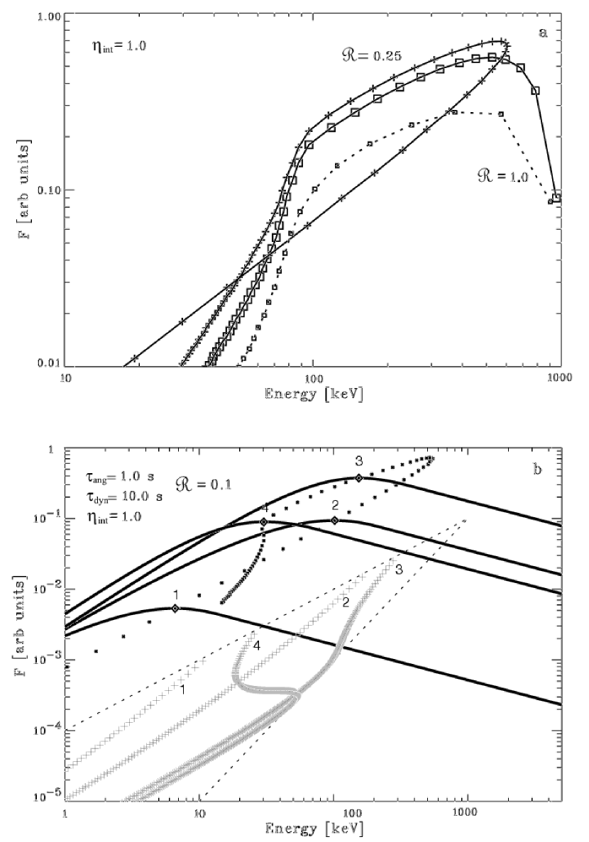
Figure 10: Variations in the spectral behavior due to the variation in the intrinsic light curve. (a) Same as figure 9 but for a Gaussian intrinsic light curve and ${{\cal{R}}}=0.25$, a one-sided, pure decay Gaussian produces a so-called hard-to-soft pulse (squares), while a symmetric Gaussian (crosses) produces a so-called tracking (hard-soft-hard) pulse. For the latter case the rise phase will follow the intrinsic HIC. For comparison, the dashed line shows the HIC for a one-sided exponential decay with ${{\cal{R}}}=1.0$ from Fig. 9b. (b) Same as Fig. 7 but for a Gaussian intrinsic light curve with equal rise and decay time scales. Circles show the HIC relation and the large crosses show the peaks of the contributing spectra. Times 1 and 2 are during the rise phase while 3 and 4 are for the decay phase.

In summary, for the intrinsic rise phase the flux will be dominated by $\theta=0$ and the HIC will follow the intrinsic $\eta_{\rm int}$. This makes the rise phase of a tracking pulse of interest as it reveals the intrinsic HIC. For the decay phase the ratio ${\cal R}$ determines the behavior. For ${\cal R}\gg 1$ the flux from $\theta_{\rm max}$ dominates and $\eta=2$, while for ${\cal R}\ll 1$ the flux is dominated by $\theta=0$ and the HIC follows $\eta_{\rm int}$. For cases in between, a HIC with $\eta=2$ dominates, for most of the observable part of the pulse, down to ${\cal R}\sim$ 0.5, the exact value depending on the intrinsic light curve shape. In general the decay phase HIC follows initially a concave curve sometimes resembling an S-shaped curve. The transition in these cases is similar but much broader than those referred to as track jumps by BR01 (the case with two parallel HIC curves displaced from each other), which was explained as two separate spectral components coming from two overlapping pulses. The S-shape feature, with a transition from $\eta=\eta_{\rm int}$ to $\eta=2$, can explain the more moderate changes seen in Figure 2, and demonstrates that the HIC shape can be used as a diagnostic for the value of ${\cal R}$ and the intrinsic light curve.

6 MODIFICATIONS OF THE BASIC MODEL

In deriving the above equations and the HIC we have made several simplifying assumptions. We therefore briefly discuss how the results are affected when we relax some of these restrictions.

6.1 Spatially Broad Emitting Region

A limitation of the results presented in §3 is the delta function representation of the spatial distribution of the emission. The actual emitting region most likely has a finite width, less or equal to the width $\Delta^{\prime}$ of the shell. Here we assume it to be equal to the shell width, with $j^{\prime}\propto g(R^{\prime},{\Delta^{\prime}})$ instead of the delta function description used in §4. The above approximation is valid for ${\Delta^{\prime}}/R\ll 1$. This can be demonstrated assuming a Gaussian distribution, $g(R^{\prime},{\Delta^{\prime}})=2/({\Delta^{\prime}}\sqrt{\pi})\exp\left[-((R^{\prime}-R)/{\Delta^{\prime}})^{2}\right]$. If we replace the $\delta(R^{\prime}-R)$ factor in equation (12) by this form and carry out the derivation again, then equation (16) becomes

$$F_{\rm bol}(t)=F_{0}\mu\frac{{\cal{D}}^{2}(\mu)}{\Gamma^{2}}\left(1+\frac{{\Delta^{\prime}}}{\sqrt{\pi}R}\right)$$ (23)

If the relation between $\Delta^{\prime}$ and $R$ is the one given by equation (6) this becomes $F(t)\sim F_{0}\mu({\cal{D}}/\Gamma)^{2}(1+1/\Gamma)$, which shows that the width of the spatial distribution affects the flux (negligible for $\Gamma\gg 1$) but has no effect at all on the spectrum of the emission.

6.2 Geometrical Effects

Another tacit assumption has been that the emission surface is spherical, either forming a complete sphere or, if it is confined into a jet of opening angle $\theta_{\rm jet}$, that the LOS intersects the jet at an angle more than $1/\Gamma$ from the edge of the jet. If the LOS is close to the edge of the jet then an extra steepening of the HIC can arise, apart from the nominal value for the angular spreading case ($\eta=2$). Let us consider this effect for the delta function emission, or ${\cal{R}}\rightarrow\infty$. During the early stages of the pulse an observer will see full $(2\pi)$ annuli with $E_{\rm p}$ and $F$ varying as described in §4. However, when the azimuthal symmetry is broken, i.e. the annuli are no longer whole, the flux integrated over the partial annuli will be less compared to what is expected from a full annulus. However, the observed value of the $E_{\rm p}$ will not be effected as the spectrum will not change. This will lead to a break in the HIC, from $\eta=2$ to a larger $\eta$. A corresponding behavior will also be seen in the light curve. This could explain the most extreme cases in the BR01 sample.

6.3 Inhomogeneities

In the description of the relativistic outflow we have assumed that the angular distribution of the Lorentz factor is homogeneous, i.e., it is constant over the angles $\theta$ and $\phi$ and that at angles larger than $\theta_{\rm jet}$, $\Gamma$ drops abruptly to zero. However, this is just a simplistic description and does not necessarily describe the actual situation. Deviations are most probably important at the edges of the jet. Therefore, if the beaming angle is of the same size as the jet opening angle and/or if the LOS is close to its edge, then the intensity will be affected. A variable Lorentz factor will give rise to a slight deviation from spherical symmetric outflow. This will affect only the shape of the light curve and the time evolution of the observed $E_{\rm p}$, but not the HIC because both $F$ and $E_{\rm p}$ will be affected same way.

6.4 Spectral Variations

We have also not considered the effects of the intrinsic, rest frame, spectral-shape variation (changes in $\alpha$ and $\beta$) during the pulse, but have rather concentrated on the exploration of the variation of $E_{\rm p}$ and flux. As shown above, there is a softening that occurs naturally in this scenario and hence could be one of the reasons for the observed softening without the intrinsic spectrum necessarily changing. For a more general study, individual cases need to be examined. This emphasizes again that the interpretation of the observed spectra and their relation to the source spectrum, and consequently the emission mechanism, is not straightforward. This aspect of the problem is, however, beyond the scope of this paper, but will be dealt with in a future paper.

7 SUMMARY AND DISCUSSION

We have examined the effect of differences in light travel time due to the curvature of the expanding shell and determined to what extent it can affect the width and shape of pulses and their spectral time evolution. The energy flux $F$ and the photon energies $E$ will be affected by the angle-dependent Lorentz-boost factor $\cal{D(\mu)}$; $F\propto{\cal{D}}^{2}$ and $E\propto{\cal{D}}$. The peak energy of the $\nu F_{\nu}$ spectra, $E_{\rm p}$, will thus follow a hardness-intensity correlation (HIC) $F\propto E^{\eta}$ with $\eta=2$. Furthermore, the decay phase of a pulse will follow the form $(1+t/\tau_{\rm ang})^{2}$. We show that this effect should be important for a reasonable choice of parameters (Lorentz factor, burst energy, shell width etc.) and that these characteristics agree with the average behaviors found in pulses.

However, the curvature effect can not alone explain the large observed dispersion of the HIC index $\eta$ . Cases with $\eta$ largely different from $2$ we believe are produced by a finite dynamic time, $\tau_{\rm dyn}\neq 0$. The resulting spectral/temporal behavior depends mainly on the ratio ${\cal{R}}=\tau_{\rm ang}/\tau_{\rm dyn}$. The intrinsic HIC (assumed to be a power law with an intrinsic index $\eta_{\rm int}$) will be revealed when ${\cal{R}}<0.5$ while the behavior expected from the curvature effect with a HIC index $\eta=2$ will dominate for ${\cal{R}}>2$. For intermediate ${\cal{R}}$s the $F-E_{\rm p}$ relation will deviate from a pure power-law, having a more concave shape (in a $\log-\log$ plot). A general softening of the spectra with time, which has been observed, is also expected, independent of any changes in the intrinsic spectrum, and therefore independent of the physical environment where the pulses are produced.

An important conclusion of this work is that one must be very careful in the interpretation of the observed light curves and spectra, their parameters and evolution. This is because we have shown that the observed light curve will in most cases be different from the intrinsic one and the observed spectra will have a complex relation to the intrinsic ones. The spectra in the observer frame will be broader and, for instance, the low-energy power-law slopes $\alpha$ will be softer than the intrinsic ones. In some cases, flat-topped spectra are produced which, in the observer frame, appear to have either $\alpha$ or $\beta=-1$. Furthermore, we also explain the occurrence of pulses whose $E_{\rm p}$ track the flux up, and down, during the rise and decay phase, respectively, as well as the occurrence of pulses where the hardness declines monotonically independent of the rise and fall of the flux.

Ultimately, we wish to determine the characteristics of the intrinsic emission, namely $F^{\prime}(t)$, $E_{\rm p}^{\prime}(t)$, $\eta_{\rm int}$, and if possible the spectral power law slopes $\alpha$ and $\beta$. In addition, we want to determine the distance $R$ from the progenitor where the fireball emits the $\gamma$-rays and to discern something about the shell width $\Delta^{\prime}$ and/or its spreading. Fits to the HIC and observed light curve will be able to reveal ${\cal{R}}$ and $F^{\prime}(t)$. Below we discuss the principle diagnostics that can be made for three different situations. The value of the bulk Lorentz factor $\Gamma$ remains an unknown parameter.

Case I. The observed HIC is a pure $\eta=2$ power law (e.g. pulses in Fig.1): According to our model the curvature effect is dominant (It could, however, also be due to an intrinsic $\eta=2$ HIC). The observed light curve will (asymptotically) follow equation (2) with $d=2$, from which one can determine the value of $\tau_{\rm ang}$. This time constant determines the distance at which the shell lights up:

$$R=2\tau_{\rm ang}\Gamma^{2}v=6\times 10^{14}{\rm cm}\left(\frac{\tau_{\rm ang}}{1\rm{s}}\right)\left(\frac{\Gamma}{10^{2}}\right)^{2}\beta$$ (24)

The observed light curve can, in principle, be deconvolved, with equation (17) as the impulse response, to obtain $F^{\prime}(t)$. A better knowledge of $F^{\prime}(t)$, then gives a more accurate value of ${\cal{R}}$ (and thereby $\tau_{\rm dyn}$) from a fit to the HIC. Knowing $\tau_{\rm dyn}$ one can put constraints on $\Delta^{\prime}/{\beta_{\rm sh}}^{\prime}$ or ${\beta_{\rm sh}}^{\prime}(\Gamma_{\rm s}/\Gamma$). Furthermore, the observed, instantaneous spectra will be results of integrations of the intrinsic spectra along a $\eta=\eta_{\rm int}$ power law. Combining this knowledge with the observations could reveal $E_{\rm p}^{\prime}(t)$ and $\eta_{\rm int}\sim\alpha_{\rm obs}$ and possibly $\alpha_{\rm int}$.

Case II. The HIC is a pure power law with index $\eta$, substantially different from $2.0$ (e.g. pulse in Fig. 2d): Here, $\eta=\eta_{\rm int}$ and the light curve should reflect the intrinsic $F^{\prime}(t)$ (smoothed somewhat by the curvature effect). The energy evolution follows $E_{\rm p}^{\prime}(t)$. Using $F^{\prime}(t)$ a more thorough fit of the HIC can be made giving ${\cal{R}}$, which gives an estimate of $R{\beta_{\rm sh}}^{\prime}/\Delta^{\prime}$ or ${\beta_{\rm sh}}^{\prime}(\Gamma_{\rm s}/\Gamma)$ (independent of $R$). The spectra arise from integrations along $\eta=2$ which, depending on the details of the case, maybe provide a possibility to determine $\alpha_{\rm int}$.

Case III. Intermediate cases where S-curves are seen (e.g. pulses in Figs. 2a, b, and c): The low energy section of the HIC (i.e. at late times) will follow $\eta=2$ and gives the value of $\tau_{\rm ang}$ and $R$. With this knowledge the light curve can be deconvolved and $F^{\prime}(t)$ can be found. A fit to the HIC can now be made to find ${\cal{R}}$ [which gives $\tau_{\rm dyn}$ and $\Delta^{\prime}$] and $\eta_{\rm int}$ which will be revealed from the early part, [which will allow the determination of $E^{\prime}(t)$]. A corresponding softening of the spectra as described in the paper should be present.

BR01 found that in several GRBs, with two separable pulses, the HIC index varied less from pulse to pulse in a single burst as compared to its variation in different bursts. This requires that the pulses in multi-pulse bursts be produced in shocks created in a similar environment, with similar values of $R$, $\Gamma_{\rm rel}$, $\Gamma$, ${{\cal{R}}}$, $\eta_{\rm int}$, $n$ and $B$. This could happen in a scenario in which the two long pulses are created as two similar shells catch up with a leading, slower, more bulky shell that has already been significantly decelerated due to interaction with the circumburst environment. Such pulses then occur approximately within the same environment, at roughly the same distance $R$ (therefore same $\tau_{\rm ang}$) and $\Gamma_{\rm rel}$. This scenario also increases the value of $\Gamma_{\rm rel}$, which implies a higher magnetic field, radiative efficiency, and a minimum electron Lorentz factor, and a higher synchrotron peak frequency:

$$h\nu_{\rm s}=\frac{3e}{4\pi m_{\rm e}c}\Gamma B\gamma_{\rm e}^{2}=5{\rm eV}(\Gamma_{\rm rel}-1)^{2.5}\left(\frac{R}{10^{15}{\rm cm}}\right)^{-1},$$ (25)

where we have used the relations for B and $\gamma_{\rm e}$ described at the beginning of §3. With $\Gamma_{\rm rel}\sim 100$, $h\nu_{\rm s}=500$ keV, so that the expected synchrotron spectrum will peak in the BATSE window and will require no additional boost, for instance, from Compton upscattering as in the Synchrotron-Self-Compton model (SSC) (Panaitescu & Mészáros, 2000). This scenario is similar to that of the external shock model normally proposed for the generation of the afterglows, which has difficulty to explain the prompt gamma-ray emission because of its high variability (Fenimore et al., 1996). However, the GRBs discussed in this paper are smooth with few pulses and do not exhibit the high variability of more complex bursts, so that this objection is not applicable.

References

- Band et al. (1993) Band, D., et al. 1993, ApJ, 413, 281
- Borgonovo & Ryde (2001) Borgonovo, L., & Ryde, F. 2001, ApJ, 548, 770
- Borgonovo et al. (2002) Borgonovo, L., Ryde, F., de Val Borro, M., & Svensson, R. 2002, in the proceedings of ’Gamma-Ray Burst and Afterglow Astronomy 2001’, Woods Hole, MA, in press
- Crider et al. (1997) Crider, A., et al. 1997, ApJ, 479, L39
- Eriksen & Grøn (2000) Eriksen, E., & Grøn, Ø. 2000, Amer. J. Phys., 68, 1123
- Fenimore et al. (1996) Fenimore, E. E., Madras, C. D., & Nayakshin, S. 1996, ApJ 473, 998
- Fenimore & Sumner (1997) Fenimore, E., & Sumner, M. C. 1997, All-Sky X-Ray Observations in the Next Decade, 167
- Fishman et al. (1994) Fishman, G. J., et al. 1994, ApJS, 92, 229
- Ford et al. (1995) Ford, L. A., et al. 1995, ApJ, 439, 307
- Frail et al. (2001) Frail, D. A., et al. 2001, ApJ, 562, L55
- Gissellini et al. (2000) Gisellini, G., Celotti, A., & Lazzati, D. 2000, MNRAS, 313, L1
- Granot et al. (1999) Granot, J., Piran, T., Sari, R. 1999, ApJ, 513, 679
- Golenetskii et al. (1983) Golenetskii, S. V., Mazets, E. P., Aptekar, R. L., & Ilyinskii, V. N. 1983, Nature, 306, 451
- Kargatis et al. (1995) Kargatis, V. E., et al. 1995, A&SS, 231, 177
- Kocevski & Liang (2001) Kocevski, D., & Liang, E. 2001, in AIP Conf. Proc. 586, Relativistic Astrophysics: 20th Texas Symposium, ed. J. C. Wheeler, & H. Martell (New York: AIP), 623
- Lee et al. (2000a) Lee A., Bloom, E. D., & Petrosian, V. 2000a, ApJS, 131, 1
- Lee et al. (2000b) Lee A., Bloom, E. D., & Petrosian, V. 2000b, ApJS, 131, 21
- Liang (1997) Liang, E. P. 1997, ApJ, 491, L15
- Liang & Kargatis (1996) Liang, E. P., & Kargatis, V. E. 1996, Nature, 381, 495
- Lloyd & Petrosian (2000) Lloyd, N., & Petrosian, V. 2000, ApJ, 543, 722
- Lloyd & Petrosian (2002) Lloyd, N., & Petrosian, V. 2002, ApJ, 565, 182
- Lyutikov & Blackman (2001) Lyutikov, M. & Blackman, E. G. 2001, MNRAS 321, 177
- Norris et al. (1996) Norris, J. P., Nemiroff, R. J., Bonnell, J. T., Scargle, J. D., Kouveliotou, C., Paciesas, W. S., Meegan, C.A., & Fishman, G. J. 1996, ApJ, 459, 393
- Norris, Marani, & Bonnell (2000) Norris, J. P., Marani, G. F. Bonnell, J. T. 2000, ApJ, 534, 248
- Panaitescu & Mészáros (2000) Panaitescu, A., & Mészáros, P. 2000, ApJ, 544, L17
- Rees & Mészáros (1992) Rees, M. J., & Mészáros, P. 1992, MNRAS, 258, 41
- Rybicki & Lightman (1979) Rybicki, G. B., & Lightman, A. P. 1979, Radiative Processes in Astrophysics (New York: Wiley)
- Ryde, Borgonovo, & Svensson (2000) Ryde, F., Borgonovo, L., & Svensson, R. 2000, in AIP Conf. Proc. 526, Gamma-Ray Bursts, 5th Huntsville Symposium, ed. R. M. Kippen, R. S. Mallozzi, & G. J. Fishman (New York: AIP), 180
- Ryde, Kocevski & Liang (2002) Ryde, F., Kocevski, D., & Liang, E., in the proceedings of ’Gamma-Ray Burst and Afterglow Astronomy 2001’, Woods Hole, MA, in press
- Ryde & Svensson (2000) Ryde, F., & Svensson, R. 2000, ApJ, 529, L13
- Ryde & Svensson (2002) Ryde, F., & Svensson, R. 2002, ApJ, 566, 210
- Soderberg & Fenimore (2001) Soderberg, A. M. , & Fenimore, E. E. 2001, in Gamma-Ray Bursts in the Afterglow Era, ed. E. Costa, F. Frontera, & J. Hjorth (Berlin Heidelberg: Springer), 87
- Spada, Panaitescu, & Mészáros (2000) Spada, M., Panaitescu, A., & Mészáros, P. 2000, ApJ 537, 824
- Tavani (1996) Tavani, M. 1996, ApJ 466, 768