Big Bang Nucleosynthesis with Gaussian Inhomogeneous Neutrino Degeneracy

Abstract

We consider the effect of inhomogeneous neutrino degeneracy on Big Bang nucleosynthesis for the case where the distribution of neutrino chemical potentials is given by a Gaussian. The chemical potential fluctuations are taken to be isocurvature, so that only inhomogeneities in the electron chemical potential are relevant. Then the final element abundances are a function only of the baryon-photon ratio $\eta$, the effective number of additional neutrinos $\Delta N_{\nu}$, the mean electron neutrino degeneracy parameter $\bar{\xi}$, and the rms fluctuation of the degeneracy parameter, $\sigma_{\xi}$. We find that for fixed $\eta$, $\Delta N_{\nu}$, and $\bar{\xi}$, the abundances of ⁴He, D, and ⁷Li are, in general, increasing functions of $\sigma_{\xi}$. Hence, the effect of adding a Gaussian distribution for the electron neutrino degeneracy parameter is to decrease the allowed range for $\eta$. We show that this result can be generalized to a wide variety of distributions for $\xi$.

I Introduction

Many modifications to the standard model of Big Bang nucleosynthesis (BBN) have been explored [1]. One of the most exhaustively investigated variations on the standard model is neutrino degeneracy, in which each type of neutrino is allowed to have a non-zero chemical potential [2], and a number of models have been proposed to produce a large lepton degeneracy [3]-[5]. More recently, observations of the cosmic microwave background (CMB) fluctuations have been combined with BBN to further constrain the neutrino chemical potentials [6]-[11].

An interesting variation on these models is the possibility that the neutrino degeneracy is inhomogeneous [12]-[14]. The consequences of inhomogeous neutrino degeneracy for BBN were examined by Dolgov and Pagel [13] and Whitmire and Scherrer [15]. Dolgov and Pagel examined models in which the length scale of the inhomogeneity was sufficiently large to produce an inhomogeneity in the presently-observed abundances of the elements produced in BBN. Whitmire and Scherrer investigated inhomogeneities in the neutrino degeneracy on smaller scales; in these models the element abundances mix to produce a homogeneous final element distribution. Using a linear programming technique, they derived upper and lower bounds on the baryon-to-photon ratio $\eta$ for arbitrary distributions of the neutrino chemical potentials and showed that the upper bound on $\eta$ could be considerably relaxed. However, the resulting distributions for the neutrino chemical potentials were quite unnatural. Hence, in this paper, we examine a more restricted class of models, in which the distribution of the chemical potentials is taken to be a Gaussian.

In the next section, we discuss our model for inhomogeneous neutrino degeneracy. We calculate the effect of these inhomogeneities on the final element abundances and discuss our results in Sec. 3. We find that, in most cases, the effect of Gaussian inhomogeneities in the electron neutrino chemical potential is to increase the abundances of deuterium, ⁴He, and ⁷Li relative to their abundances in models with homogeneous neutrino degeneracy.

II Model for Inhomogeneous Neutrino Degeneracy

We first consider the case of homogeneous neutrino degeneracy. For this case, each type of neutrino is characterized by a chemical potential $\mu_{i}$ ($i=e,~{}\mu,~{}\tau$), which redshifts as the temperature, so it is useful to define the constant quantity $\xi_{i}\equiv\mu_{i}/T_{i}$. Then the neutrino and antineutrino number densities are functions of $\xi_{i}$:

$$n_{\nu_{i}}={1\over 2\pi^{2}}T_{\nu}^{3}\int_{0}^{\infty}{x^{2}dx\over 1+\exp(x-\xi_{i})},$$ (1)

and

$$n_{\bar{\nu}_{i}}={1\over 2\pi^{2}}T_{\bar{\nu}}^{3}\int_{0}^{\infty}{x^{2}dx\over 1+\exp(x+\xi_{i})},$$ (2)

and the total energy density of the neutrinos and antineutrinos is

$$\rho={1\over 2\pi^{2}}T_{\nu}^{4}\int_{0}^{\infty}{x^{3}dx\over 1+\exp(x-\xi_{i})}+{1\over 2\pi^{2}}T_{\bar{\nu}}^{4}\int_{0}^{\infty}{x^{3}dx\over 1+\exp(x+\xi_{i})}.$$ (3)

Electron neutrino degeneracy changes the $n\leftrightarrow p$ weak rates through the number densities given in equations (1) and (2), while the change in the expansion rate due to the altered energy density in equation (3) affects BBN for degeneracy of any of the three types of neutrinos. (See Ref. [2] for a more detailed discussion).

Now consider the effect of inhomogeneities in the neutrino chemical potential. As noted in Ref. [15], neutrino free-streaming will erase any fluctuations on length scales smaller than the horizon at any given time. Thus, in order for inhomogeneities to affect BBN, they must be non-negligible on scales larger than the horizon scale at $n\leftrightarrow p$ freeze-out, which corresponds to a comoving scale $\sim 100$ pc today. On the other hand, if the neutrino chemical potential is inhomogeneous on scales larger than the element diffusion scale, estimated in Ref. [15] to correspond to a comoving length $\sim 1$ Mpc, then the result will be an inhomogeneous distribution of observed element abundances today (the possibility considered in Ref. [13]).

To make any further progress, we need a specific distribution $f(\xi_{i})$ for neutrino chemical potentials. In analogy with the distribution of primordial density perturbations (and in accordance with the central limit theorem) we take this distribution to be a multivariate Gaussian. Such a distribution is entirely characterized by the power spectrum of fluctuations, $P(k)$. For a power spectrum of the form $P(k)\propto k^{n}$ the rms fluctuation $\sigma_{\xi}$ on a given length scale $\lambda$ is given by

$$\sigma_{\xi}\propto\lambda^{-(n+3)/2}$$ (4)

We wish to consider only cases for which the presently-observed element distribution (determined by $\sigma_{\xi}$ at a comoving scale of $\sim 1$ Mpc) is homogenous, while the distribution is highly inhomogenous on the horizon scale at nucleosynthesis (a comoving scale of $\sim 100$ pc). Since our two length scales of interest differ by a factor of $10^{4}$, this condition can be satisfied for any $k^{n}$ power spectrum with $n>-3$. For instance, for a white-noise power spectrum, $n=0$, a value of $\sigma_{\xi}=1$ at the BBN horizon scale corresponds to $\sigma_{\xi}=10^{-6}$ at the element diffusion scale.

Given these conditions, it is a good approximation to assume that BBN takes place in separate horizon volumes, with the value of $\xi$ taken to be homogeneous within each volume. At late times, the elements produced within each volume mix uniformly to produce the observed element abundances today.

We make the additional assumption that the neutrino fluctuations are isocurvature, so that the total fluctuation in energy density is zero, even when the chemical potential is inhomogeneous. This implies that the overdensity in the degenerate neutrinos is compensated by an underdensity in some other component. In Ref. [13], for example, the degeneracies in each of the three neutrinos are arranged so that the total density remains uniform. In Ref. [14], the compensation is produced by a sterile neutrino. Such models have the advantage that they produce no additional inhomogeneities in the cosmic microwave background as long as the compensating energy density does not include photons or baryons. (Note that this is not the assumption made in Ref. [15]). We also assume for simplicity that $\eta$ remains uniform in the presence of an inhomogeneous lepton distribution. With this set of assumptions, the only neutrino for which inhomogeneities in the chemical potential are important for BBN is the electron neutrino; the effect of the other neutrino chemical potentials is to alter the total energy density, which is now assumed to be homogeneous.

It has recently been noted that if the large mixing angle solution of the solar neutrino problem is correct, then neutrino flavor oscillations will cause the neutrino chemical potentials to equilibrate prior to Big Bang nucleosynthesis [16, 17, 18]. In our inhomogeneous model, the effect of this equilibration would depend on the compensation mechanism for the inhomogeneities. In models in which the fluctuations in the electron neutrino chemical potential are compensated by fluctuations in the chemical potentials of the $\mu$ and $\tau$ neutrinos, the effect of such flavor oscillations would be to erase any spatial fluctuations in the chemical potentials. In models where the electron neutrino chemical potential fluctuations are compensated in some other way, the chemical potentials of all three species would be equal at any point in space, but the spatial fluctuations would be preserved. Any large $\Delta N_{\nu}$ in this case would have to be due to some other form of energy beyond the standard three neutrinos.

III Calculations and Discussion

The model described in the previous section can be completely specified by two parameters, the (inhomogeneous) electron neutrino degeneracy parameter, $\xi_{e}$, and the additional (homogeneous) energy density due to the degeneracy of all three neutrinos plus any additional relativistic component. We parametrize the latter in terms of $\Delta N_{\nu}$, the effective number of additional neutrinos. This second parameter hides our ignorance about the compensation mechanism and about the degeneracies among the other two types of neutrinos. In our simulation, we take $\xi_{e}$ to be homogeneous within a given horizon volume during nucleosynthesis. Different horizon volumes may have different values of $\xi_{e}$, which are given by the distribution function $f(\xi_{e})$, i.e, the probability that a given horizon volume has a value of $\xi_{e}$ between $\xi_{e}$ and $\xi_{e}+d\xi_{e}$. (Since we are considering only inhomogeneities in electron neutrinos, we now drop the $e$ subscript). We take $f(\xi)$ to have a Gaussian distribution with mean $\bar{\xi}$ and rms fluctuation $\sigma_{\xi}$:

$$f(\xi)={1\over\sqrt{2\pi}\sigma_{\xi}}\exp[-(\xi-\bar{\xi})^{2}/2\sigma_{\xi}^{2}]$$ (5)

Then the final primordial element abundances, for a fixed value of $\eta$ and $\Delta N_{\nu}$, will be functions of $\bar{\xi}$ and $\sigma_{\xi}$; we can write, for a given nuclide $A$,

$$\bar{X}_{A}=\int_{-\infty}^{\infty}X_{A}(\xi)f(\xi)d\xi,$$ (6)

where $X_{A}(\xi)$ is the mass fraction of $A$ as a function of $\xi$, and $\bar{X}_{A}$ is the mass fraction of $A$ averaged over all space; after the matter is thoroughly mixed, $\bar{X}_{A}$ will be the final primordial mass fraction.

A full treatment for all possible values of $\eta$, $\Delta N_{\nu}$, $\bar{\xi}$, and $\sigma_{\xi}$ is impractical. We have chosen to concentrate on variations in the latter two quantities, since we are most interested in the effects of inhomogeneities in the chemical potential. Because of the large number of free parameters and the difficulty of exhaustively searching all of parameter space, our goal is to discern any general results which are independent of $\eta$ and $\Delta N_{\nu}$.

There are now strong limits on $\eta$ from the cosmic microwave background alone, independent of BBN. We examine two extreme values for $\eta$: $\eta=4\times 10^{-10}$ and $\eta=1\times 10^{-9}$; these represent very conservative lower and upper bounds on $\eta$ from the CMB in models with non-zero neutrino degeneracy [10]. For $\Delta N_{\nu}$, we consider $\Delta N_{\nu}=0$ and 5. Note that the first of these is only possible if the extra energy density in the degenerate electron neutrinos is compensated by a decrease in the energy density in some other relativistic component. For each of these cases, we calculate the abundances of ⁴He, D, and ⁷Li as a function of $\sigma_{\xi}$ for $\bar{\xi}=-1$ to $+1$ in steps of 0.5. Our results are displayed in Figures 1-3. In each of these figures, we also show observational limits on the primordial element abundances from Ref. [19]: $2.9\times 10^{-5}<({\rm D/H})<4.0\times 10^{-5}$, $0.228<Y_{P}<0.248$, and $-9.9<\log(^{7}{\rm Li/H})<-9.7$.

The general behavior of the element abundances in Figs. 1-3 is very clear. As expected, for $\sigma_{\xi}\ll\bar{\xi}$, the abundances of deuterium, ⁴He, and ⁷Li are unchanged from their values in the corresponding homogeneous model with the same value of $\bar{\xi}$. At the opposite limit, when $\sigma_{\xi}\gg\bar{\xi}$, the models all converge to a single limiting value; again, this is what one would naively expect. What is interesting is that, with a few exceptions, the introduction of a Gaussian distribution of values for $\xi$ results in an increase in the abundance of each element relative to the corresponding homogeneous model with the same value of $\bar{\xi}$. The only exceptions occur for ⁴He with negative values of $\bar{\xi}$, (for which $Y_{P}$ is far too large to be physically reasonable), and some of the ⁷Li curves, for which there is a tiny decrease in the ⁷Li abundance over a short range of $\sigma_{\xi}$ values.

This result may seem surprising, but it is a simple consequence of the behavior of $X_{A}(\xi)$. In particular, if $X_{A}(\xi)$ is a convex function ($X_{A}^{\prime\prime}(\xi)>0$), then Jensen’s inequality [20] gives

$$\int_{-\infty}^{\infty}X_{A}(\xi)f(\xi)d\xi>X_{A}(\bar{\xi}).$$ (7)

We find, for example, for $\Delta N_{\nu}=0$, and both values of $\eta$, that our $X(\xi)$ curves are all convex in the range $-2<\xi<2$, with the exception of ⁴He at $\xi<-1$, and ⁷Li with $\eta=1\times 10^{-9}$. These are precisely the regimes for which we observe equation (7) to fail. Of course, none of the $X_{A}(\xi)$ curves is convex for all values of $\xi$; the practical condition for equation (7) to hold is that the $X(\xi)$ curves be convex as long as $f(\xi)$ is non-negligible.

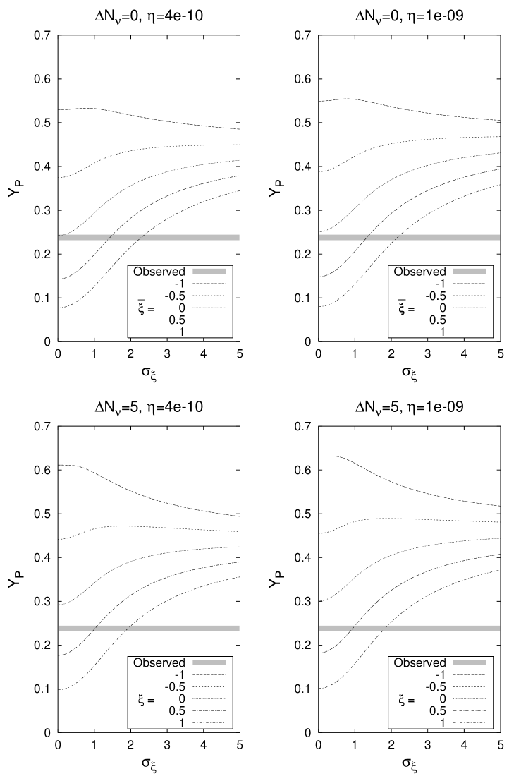
FIG. 1.: The primordial ⁴He mass fraction, $Y_{P}$, as a function of the rms fluctuation in the electron chemical potential $\sigma_{\xi}$, for the indicated value of the mean electron neutrino chemical potential $\bar{\xi}$. Each figure corresponds to the indicated value of the baryon-photon ratio $\eta$ and the effective number of extra neutrinos $\Delta N_{\nu}$. The gray shaded region gives observational limits on $Y_{P}$ from Ref. [19].

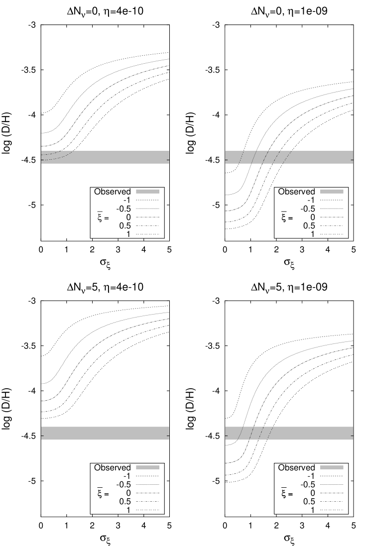
FIG. 2.: As Fig. 1, for the primordial ratio of deuterium to hydrogen, (D/H).

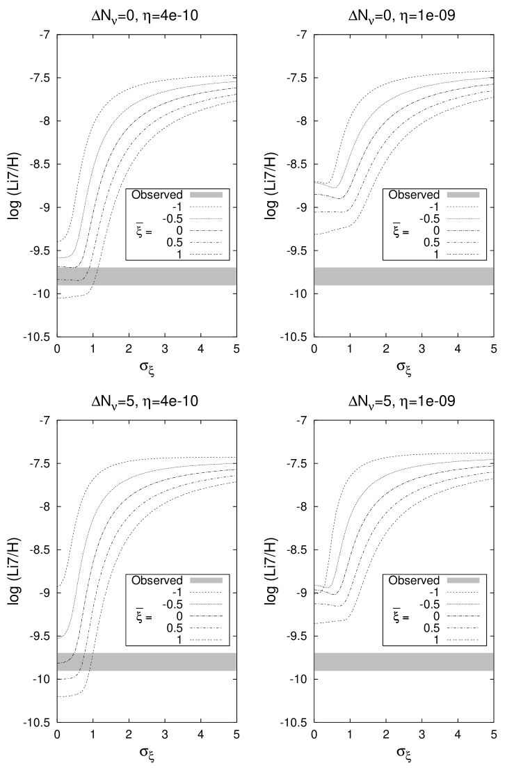
FIG. 3.: As Fig. 1, for the primordial ratio of ⁷Li to hydrogen, (⁷Li/H).

This simple behavior allows us to draw some useful general conclusions. In models in which $\xi$ and $\Delta N_{\nu}$ are allowed to vary freely, if we fix $\xi$ and trace out the allowed region in the $\eta$, $\Delta N_{\nu}$ plane, then the upper and lower bounds on $\eta$ are set primarily by the upper observational bound on ⁷Li and the upper observational limit on D, respectively, with the ⁴He limits serving primarily to set the bounds on $\Delta N_{\nu}$ [10]. However, our results indicate that the general effect of going from a homogeneous to an inhomogeneous distribution in $\xi$ is to increase both the deuterium and the ⁷Li abundances. (Again, we note a slight decrease in ⁷Li over a small range in $\sigma_{\xi}$, but this is a tiny effect). Hence, the net effect of introducing this inhomogeneity will be to decrease the allowed range for $\eta$, in comparison with the corresponding homogeneous model. This is a rare example in the study of BBN in which the introduction of an extra degree of freedom does nothing to increase the allowed range for $\eta$. Instead, the effect of adding a Gaussian distribution of values for $\xi$ is to decrease the allowed range for $\eta$.

Although we have assumed a Gaussian distribution for $\xi$, our results are much more general. In particular, as long as our distribution $f(\xi)$ is negligible over the range of values of $\xi$ for which $X_{A}(\xi)$ is not a convex function, we expect equation (7) to hold. This would apply, for example, to a top hat distribution with the same values of $\sigma_{\xi}$ as those examined here. Moreover, the distribution $f(\xi)$ need not even be symmetric for our results to apply.

Our results contrast with those of Ref. [15], which found an expanded upper limit on $\eta$ in models with inhomogeneous $\xi$. The reason for this difference is that the models examined in Ref. [15] allowed for an arbitrary distribution in $\xi$, and large increases in $\eta$ occurred for bizarre distributions in $\xi$. In particular, the distributions in Ref. [15] sampled extreme values for $\xi$, outside the range for which all of the $X_{A}(\xi)$ functions are convex.

- [1] R.A. Malaney and G.J. Mathews, Phys. Rep. C 229, 145 (1993).
- [2] R.V. Wagoner, W.A. Fowler, and F. Hoyle, ApJ148, 3 (1967); A. Yahil and G. Beaudet, ApJ206, 26 (1976); Y. David and H. Reeves, Phil. Trans. R. Soc. Lond. A 296, 415 (1980); R.J. Scherrer, Mon. Not. R. astron. Soc. 205, 683 (1983); N. Terasawa and K. Sato, ApJ294, 9 (1985); K.A. Olive, D.N Schramm, D. Thomas, and T.P. Walker, Phys. Lett. B 265, 239 (1991); H.-S. Kang and G. Steigman, Nucl. Phys. B 372, 494 (1992); K. Kohri, M. Kawasaki, and K. Sato, ApJ490, 72 (1997).
- [3] A. Casas, W.Y. Cheng, and G. Gelmini, Nucl. Phys. B 538, 297 (1999).
- [4] J. McDonald, Phys. Rev. Lett.84, 4798 (2000).
- [5] J. March-Russell, H. Murayama, and A. Riotto, JHEP 11, 015 (1999).
- [6] J. Lesgourgues and M. Peloso, Phys. Rev. D62, 081301 (2000).
- [7] M. Orito, T. Kajino, G.J. Mathews, and R.N. Boyd, Ap.J., submitted, astro-ph/0005446.
- [8] S. Esposito, G. Mangano, G. Miele, and O. Pisanti, JHEP 9 038 (2000).
- [9] S. Esposito, G. Mangano, A. Melchiorri, G. Miele, and O. Pisanti, Phys. Rev. D63 043004 (2001).
- [10] J.P. Kneller, R.J. Scherrer, G. Steigman, and T.P. Walker, Phys. Rev. D64, 123506 (2001).
- [11] M. Orito, T. Kajino, G.J. Mathews, and Y. Wang, astro-ph/0203352.
- [12] A.D. Dolgov, Phys. Rep. C 222, 309 (1992).
- [13] A.D. Dolgov and B.E.J. Pagel, New Astron. 4, 223 (1999); A.D. Dolgov, in Particle Physics and the Early Universe (COSMO-98), edited by D.O. Caldwell, (AIP, New York, 1999).
- [14] P. Di Bari, Phys. Lett. B 482, 150 (2000); P. Di Bari and R. Foot, Phys. Rev. D63, 043008 (2001).
- [15] S.E. Whitmire and R.J. Scherrer, Phys. Rev. D 61, 083508 (2000).
- [16] C. Lunardini and A. Yu. Smirnov, Phys. Rev. D 64, 073006 (2001).
- [17] A.D. Dolgov, S.H. Hansen, S. Pastor, S.T. Petcov, G.G. Raffelt, and D.V. Semikoz, Nucl. Phys. B 632, 363 (2002).
- [18] K.N. Abazajian, J.F. Beacom, and N.F. Bell, astro-ph/0203442.
- [19] K.A. Olive, G. Steigman, T.P. Walker, Phys. Rep. 333, 389 (2000).
- [20] W. Feller, An Introduction to Probability Theory and Its Applications, Vol. II (Wiley, New York, 1971).