How fast could a proto-pulsar rotate?

Abstract

According to two estimated relations between the initial period and the dynamo-generated magnetic dipole field of pulsars, we calculate the statistical distributions of pulsar initial periods. It is found that proto-pulsars are very likely to have rotation periods between 20 and 30 ms, and that most of the pulsars rotate initially at a period $<60$ ms.

1 Introduction

Pulsars provide us an unusual physical condition to increase our knowledge of the nature. As yet, one of the essential parameters, the initial periods $P_{0}$ of proto-pulsars,which may reveal precious information of dynamical supernova process, are poorly known. Actually there are 3 efforts to estimate $P_{0}$ in the literatures. 1, The period $P_{0}$ can be found via $T=P/[(n-1)\dot{P}][1-(P_{0}/P)^{n-1}]$ if the age $T$ and the braking index $n\equiv{\Omega\ddot{\Omega}/\dot{\Omega}^{2}}$ ($\Omega=2\pi/P$ the angular velocity of rotation) are measured (e.g., Kaspi et al. 1994), where $P$ is the rotation period observed. This method needs constant braking indices, which are likely to vary with time (Xu & Qiao 2001). 2, Monte Carlo simulation is used to study the pulsar “current” in the magnetic field - period diagram (e.g., Lorimer et al. 1993); the initial period of “injected” pulsars into the population are adjusted so as to sustain the number of pulsars observed at longer periods. 3, Initial periods can be inferred for pulsars that reside within composite supernova remnants which are powered by the pulsar spindown energy (van der Swaluw & Wu 2001). The derived $P_{0}$ via these 3 ways are 10-60 ms, $\sim 300$ ms, and 37-82 ms (sometimes several hundred milliseconds), respectively. In addition, Lai et al. (2001) studied the implication of the apparent spin-kick alignment in the Crab and Vela pulsars, and found that the initial period should be $\lesssim 1$ ms in both the electromagnetic rocket model and the hydrodynamic natal model, or $<10$ s in the asymmetric neutrino emission model, in order to produce a high kick velocity.

In this paper, we try an alternative effort to derive the initial period through a relation between the initial period and the dynamo-originated magnetic field of pulsars. The magnetic field $B$ is assumed not to change in our discussion, since both observation and theory imply that a pulsar’s $B$-field does not decay significantly during the rotation-powered phase (Bhattacharya et al. 1992 and, e.g., Xu & Busse 2001). Therefore the field strength observed for a normal pulsar represents its initial value. On another hand, the strong magnetic field is supposed to be created by dynamo action during the proto-pulsar stage (Thompson & Duncan 1993, Xu & Busse 2001). We may obtain the initial period if we can find an estimated relation between $B$ and $P_{0}$ during the dynamo episode.

2 The model for calculation of pulsar initial periods

2.1 The model

Dynamo action may occur during the first a few seconds of both neutron stars and strange stars (Thompson & Duncan 1993, Xu & Busse 2001). In the magnetohydrodynamic (MHD) mean field dynamo theory, the helical turbulence (leading to the $\alpha$ effect), differential rotation (the $\Omega$ effect), and the turbulent diffusion (the $\beta$ effect) are combined (e.g., Moffatt 1978, Blackman 2002). The dynamo-created magnetic fields are complex and not very certain for specific astrophysical processes due to the nonlinearity of the MHD equations. Nevertheless it is generally believed (Blackman 2002 and references therein) that a seed field begins to grow kinematically until a saturation (energy equipartition between field and fluid) phase when the growth slows down due to the back action of field on fluid in a small scale (at or below a typical length of turbulent eddies).

The dynamo-originated field energy in this small scale is provided by both of convection and differential rotation. The differential rotation energy is $E_{\rm dif}\sim 10^{46}P_{0}^{-2}$ erg (from eqs.(8) and (37) of Xu & Busse 2001). For proto-strange stars, the convection energy is $E_{\rm con}\sim 4\pi R^{2}L\rho v^{2}\sim 10^{48}v_{8}^{2}$ erg (Xu & Busse 2001), where $R\sim 10^{6}$ cm is the stellar radius, $L\sim 10^{5}$ cm the convective thickness, $\rho\sim 4\times 10^{14}$ g/cm³ the density of strange quark matter, and the convective velocity $v=v_{8}\times 10^{8}$ cm/s could be either $\sim 10^{8}$ cm/s for a large-scale convection or $\sim 10^{5}$ cm/s for a local turbulent eddy. For proto-neutron stars, a similar estimate gives $E_{\rm con}\sim 10^{48}$ erg (Thompson & Duncan 1993). We assume that the differential rotation energy dominates, and thus neglects the convective energy, during the episode when dynamo action works, since $E_{\rm dif}\gtrsim E_{\rm con}$ as long as $P_{0}\lesssim 100$ ms. The saturation magnetic field in small scale, $B_{\rm sat}$, satisfies

$${B_{\rm sat}^{2}\over 8\pi}\sim{E_{\rm dif}\over R^{3}}.$$ (1)

Since $E_{\rm dif}\propto P_{0}^{-2}$, we come to

$$B_{\rm sat}=AP_{0}^{-1},$$ (2)

where $A$ is a constant for a pulsar-like compact star with typical mass and radius.

The growth of a much large scale magnetic field (e.g., the observed dipole one, $B_{\rm d}$) by the $\alpha$ effect only is almost impossible because the magnetic helicity conservation eventually leads to a so called “catastrophic” quenching. Nonetheless, differential rotation may play a great role to generate large scale fields since it can regenerate a larger scale toroidal field. Assuming that the dipole magnetic field, $B_{\rm d}$, is a constant fraction of the saturation one, we have

$$B_{\rm d}=aP_{0}^{-1}.$$ (3)

However, it is possible that the ratio of $B_{\rm d}$ to $B_{\rm sat}$ is a function of $P_{0}$. The Rossby number, $R_{\rm o}=P_{0}/\tau_{\rm con}$ (the convective overturn time $\tau_{\rm con}\sim 1$ ms for both proto-neutron stars and proto-strange stars), is an effective dimensionless number to describe the importance of rotation, and may also be representative of differential rotation. Therefore the ratio may depend on a function of $R_{\rm o}$ since differential rotation is essential for large sale field generation. Observationally, the magnetic activity, which reflects the field strength in the atmospheres, of G-M dwarf stars correlate with $R_{\rm o}^{-0.55\pm 0.10}$ (Simon 1990). Considering eq.(2), we can thus assume

$$B_{\rm d}=a^{\prime}P_{0}^{-1.5}.$$ (4)

Eqs.(3) and (4) are two estimated relations between field and initial period, which will be used respectively to derive pulsar initial period in section 2.2.

After the proto-pulsar phase when dynamo action works, a pulsar may spindown because of the braking torques due to magnetodipole radiation and the unipolar generator (Xu & Qiao 2001), with a rate

$${\dot{\Omega}}=-{2R^{6}B_{\rm d}^{2}\over 3c^{3}I}\Omega^{3}\eta,$$ (5)

where $I\sim 10^{45}$ g cm² the momentum of inertia, $\eta\in(1,3)$ being a function of $B_{\rm d}$, $P$, and inclination angle $\alpha$. For the simplicity, we assume $\eta=1$ in this paper, which is also the case of conventional magnetic dipole model for pulsars with $\alpha=90^{\rm o}$. We then have the magnetic field $B_{12}=B_{\rm d}\times 10^{12}$ G by

$$B_{12}={1\over 10^{12}}\sqrt{3Ic^{3}P\dot{P}\over 8\pi^{2}R^{6}}=3.2\times 10^{7}\sqrt{P\dot{P}},$$ (6)

The magnetic field is assumed not to change; the field in eq.(6) is thus the same as in eqs.(3) and (4), by which the initial period can be obtained.

We can also have the rotation period $P(t)$ as a function of time $t$, by integrating eq.(5)

$$P(t)^{2}=P(0)^{2}+\zeta B_{12}^{2}t,$$ (7)

where $P(0)=P_{0}$, and

$$\zeta={16\pi^{2}R^{6}10^{24}\over 3c^{3}I}\simeq 1.95\times 10^{-15}~{}{\rm s}.$$

Time derivative of eq.(7) leads to $\zeta B_{12}^{2}=2P(t)\dot{P}(t)$, we then have the age $T$,

$$T={P^{2}-P_{0}^{2}\over 2P\dot{P}}.$$ (8)

Eq.(7) may be useful to study pulsar “current” in the $P-\dot{P}$ diagram.

2.2 Calculations based on pulsar data

There are three approaches to obtain pulsar ages. The first is the characteristic age $\tau=P/2\dot{P}$, which could be derived from eq.(8) if $P_{0}\ll P$. Second, for a pulsar associated with a supernova remnant (SNR), the kinematic age of the SNR could be regarded as an estimation to the pulsar age. Third, when an SNR is identified to be the remnant of a historically recorded supernova, the age of the pulsar within the SNR is then precisely known.

Among the youngest pulsars which locate in SNRs (see table 2 of Camilo et al. 2002), only the Crab pulsar is confidently believed to be associated with SN1054, the other two, PSR J1181-1926 (in the SNR G11.2-0.3) and PSR J0205+6449 (in the SNR 3C58) are suggested to be probably associated with SN1181 and possibly with SN386, respectively (Clark & Stephenson 1976). Therefore, only the real age of the Crab pulsar is exactly known in all the discovered pulsars.

For the Crab pulsar, with $P=33.4$ ms, $\dot{P}=4.2\times 10^{-13}$ s/s and $T=948$ yr, its initial period is then $P_{0}=16.8$ ms through eq.(8). Calibrated by the Crab pulsar, eq.(3) can then be rewritten as

$$B_{12}=0.0637P_{0}^{\rm-1},$$ (9)

which provides a way to calculate the initial period. The ATNF pulsar catalogue has released $\sim$1,300 radio pulsars with $P$ and $\dot{P}$ measured (http://www.atnf.csiro.au/research/pulsar/catalogue). In our calculation, millisecond pulsars are excluded, for their magnetic fields may decay significantly during the recycling phase. In this paper, the criteria used to exclude a millisecond pulsar is (a) $P\lesssim 60$ ms, (b) $T\lesssim 10^{9}$ years, and (c) $B\sim 10^{8-9}$ G. Besides millisecond pulsars, those pulsars in binary systems and those having negative values of $\dot{P}$ are also excluded. Totally 1,069 pulsars are selected for our calculation.

The initial periods are derived via eqs.(6) and (9). The result is presented by the histograms for $P_{0}$ (left panel of Fig.1). It is found that 60% pulsars have initial period less than 60 ms, exhibiting an peak at the interval 20-30 ms, as shown in Fig.1. It is worth noting that data of 997 pulsars are shown in the histogram. For the other 72 pulsars, the calculated $P_{0}$ is greater than $P$, hence results in a negative value of $T$, which means that eq.(9) may not be applicable to these pulsars.

Similarly we can also find the coefficient $a^{\prime}=8.24\times 10^{-3}$ in eq.(4) by the Crab pulsar calibration. Employing this relation, the initial periods are calculated, which is presented in the right panels of Fig.1. There are 23 pulsars which have negative calculated $T$, so that totally 1046 pulsars are plotted in the histograms. The distribution peak of $P_{0}$ is also between 20 and 30 ms, but more pulsars tend to have smaller $P_{0}$. Statistically, the distributions of characteristic age $\tau$ and the age $T$ do not show significant difference. This is not surprising since most pulsars have their initial period $P_{0}\ll P$.

3 Conclusion and discussion

The statistical distributions of pulsar initial periods are inferred based on the estimated relation between the initial periods and the magnetic dipole magnetic fields. It is found that proto-pulsars are very likely to have rotation periods between 20 and 30 ms, and that most of the pulsars rotate initially at a period $<60$ ms. The pulsar initial periods derived in this way are comparable with the previous estimates by the first and the third methods, but are significantly smaller than that by the second method (section 1).

When looking at the pulsar distribution in the $P-\dot{P}$ diagram, one generally concludes that the magnetic fields decays at a time scale of $10^{6-7}$ years since the number density of pulsars with low fields and old ages are larger than that of pulsars with high fields and young ages. However, calculations of ohmic decay of dipolar magnetic fields by Sang & Chanmugam (1987) suggest that neutron star magnetic fields may not decay significantly during the rotation-powered phases. The field of a strange star can also hardly decay because of the high magnetic Reynolds number and possible color superconductivity (e.g., Xu & Busse 2001). Observations indicate that the field decays only if the pulsar is in the accretion phase (e.g., Taam & van den Huevel 1986). If the field does not change significantly, how can we understand the apparent “field decay” in the $P-\dot{P}$ diagram? We may explain this discrepancy by studying pulsar current in the $P-\dot{P}$ diagram, according to eq.(7) with the inclusion of $\eta\neq 1$ in different emission models. Certainly the braking index varies when a pulsar evolves in this way. Further studies on this topic will be necessary and interesting.

There are a few pulsars which have initial periods $\lesssim 5$ ms in our calculation; for instance, 5 pulsars with $P_{0}<5$ ms appear in the right histogram of Fig.1 based on eq.(4). This result can not be understood in the conventional opinion of $r-$mode instability, if it is not caused by statistical error or other factors being inherent in our $P_{0}$ calculations. However, as addressed in Xu & Busse (2001), the $r-$mode instability may be inhibited by differential rotation and strong magnetic field; the problem could thus be solved.

Acknowledgments: This work is supported by National Nature Sciences Foundation of China (10173002) and the Special Funds for Major State Basic Research Projects of China (G2000077602). RXX wishes to sincerely acknowledge Mrs. S.Z. Peng for her help in preparing pulsar data two years ago.

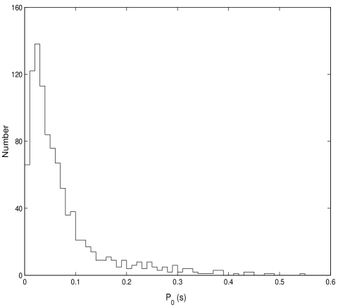
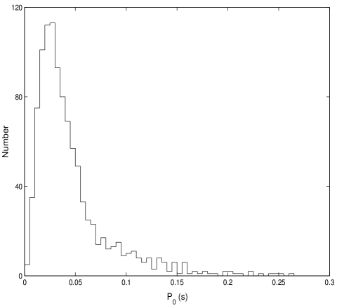
Figure 1: Histograms for the initial period $P_{0}$. Left: $P_{0}$ is calculated from $B_{12}=0.0637P_{0}^{\rm-1}$, in which data of 997 pulsars are used and each bin represents an interval of 10 ms. Right: $P_{0}$ is calculated from $B_{12}=8.24\times 10^{-1.5}P_{0}^{\rm-1.5}$, in which data of 1046 pulsars are plotted and each bin represents 5 ms.

References

- (1) Andersson, N., Kokkotas, K.D. 2001, Int. J. Mod. Phys., D10, 381
- (2) Bhattacharya, D., et al. 1992, A&A, 254, 198
- (3) Blackman, E. G. 2002, in Turbulence and Magnetic Fields in Astrophysics, ed. E. Falgarone & T. Passot, Springer Lecture Notes in Physics, in press (astro-ph/0205002)
- (4) Camilo, F., Manchester, R.N., Gaensler, B.M., Lorimer, D.R., Sarkissian, J. 2002, ApJL, in press (astro-ph/0201384)
- (5) Clark, D. & Stephenson, F. 1976, Quarterly Journal R.A.S., 17, 290
- (6) Kaspi, V. M., Manchester, R. N., Siegman, B., Johnston, S., Lyne, A. G. 1994, ApJ, 422, L83
- (7) Lai, D., Chernoff, D. F., Cordes, J. M. 2001, ApJ, 549, 1111
- (8) Lorimer, D. R., Bailes, M., Dewey, R. J., Harrison, P. A. 1993, MNRAS, 263, 403
- (9) Moffatt, H.K. 1978, Magnetic field generation in electrically conducting fluids, Cambridge Univ. Press
- (10) Sang, Yeming, Chanmugam, G. 1987, ApJ, 323, L61
- (11) Simon, T. 1990, ApJ, 359, L51
- (12) Taam, R.E., van den Huevel, E.P.J. 1986, ApJ, 305, 235
- (13) Thompson, C., Duncan, R.C. 1993, ApJ, 408, 194
- (14) van der Swaluw, E., Wu, Y. 2001, ApJ, 555, L49
- (15) Xu, R.X 2001, Science & Technology Review, Vol. 155, No. 5, 6 (in Chinese)
- (16) Xu, R.X., Busse, F.H. 2001, A&A, 371, 963
- (17) Xu, R.X., Qiao, G.J. 2001, ApJ, 561, L85