A box-fitting algorithm in the search for periodic transits

We study the statistical characteristics of a box-fitting algorithm to analyze stellar photometric time series in the search for periodic transits by extrasolar planets. The algorithm searches for signals characterized by a periodic alternation between two discrete levels, with much less time spent at the lower level. We present numerical as well as analytical results to predict the possible detection significance at various signal parameters. It is shown that the crucial parameter is the effective signal-to-noise ratio — the expected depth of the transit divided by the standard deviation of the measured photometric average within the transit. When this parameter exceeds the value of 6 we can expect a significant detection of the transit. We show that the box-fitting algorithm performs better than other methods available in the astronomical literature, especially for low signal-to-noise ratios.

1 Introduction

A considerable fraction of the periodic astronomical time series can be modeled rather accurately by finite sums of sinusoidal components. In general, these Fourier-sums have a single dominant component, and therefore the basic method of Discrete Fourier Transformation (DFT) has become commonplace in almost all applications (e.g., Deeming 1975). When the signal becomes distorted by higher harmonics (e.g., light curves of fundamental mode RR Lyrae and $\delta$ Cephei stars), this simple approach fails to perform properly, due to leakage of the signal power to many higher harmonics. One way to deal with this problem is to use a multifrequency Fourier fit for better approximation of the signal shape and thereby to increase the algorithm efficiency, a method recently suggested by Defaÿ, Deleuil & Barge (2001) for the search for extrasolar planetary transits. Another generally accepted approach is the so-called Phase Dispersion Minimization (PDM), which searches for the best period that yields the ‘smoothest’ folded time series.

Application of variants of the PDM method in the analyses of variable star observations goes back to earlier times than that of the DFT. This is primarily because the PDM algorithm does not require the computation of trigonometric functions, which put a heavy load on the computers, especially in those early days. The most frequently cited implementation of the PDM idea is that of Stellingwerf (1978). However, earlier versions had appeared already in the ’60s and early ’70s, like those of Lafler & Kinman (1965, hereafter the L-K method), Jurkevich (1971) and Warner & Robinson (1972, hereafter the W-R method). Actually, it can be shown that up to a frequency- (or trial period-) independent constant, the method of Jurkevich (1971) is equivalent to that of W-R (see, Kovács 1980). Furthermore, without the additional feature of overlapping bin structure, the method of Stellingwerf (1978) is equivalent to that of Jurkevich (1971).

The study of the algorithm presented in this paper has been stimulated by the increasing interest in searching for periodic transits by extrasolar planets (e.g., Gilliland et al. 2000; Brown & Charbonneau 2000; Udalski et al. 2002), which follow the discovery of the transit of HD 209458 (Charbonneau et al. 2000; Henry et al. 2000) by its planetary companion (Mazeh et al. 2000). Due to the short duration of the transit relative to the orbital period (typically less than 5%), the signal expected is extremely non-sinusoidal. Considering the shallowness of the transit (typically less than 2% in the case of Jupiter-size planets) and the expected high noise level of the ground-based small telescopes capable of performing large-scale surveys (e.g., Borucki et al. 2001), we suggest an algorithm that utilizes the special form of the signal. The algorithm studied here (see also Gilliland et al. 2000 and Udalski et al. 2002) is based on direct Least Squares (LS) fits of step functions to the folded signal corresponding to various trial periods. We present numerical simulations as well as analytical considerations to estimate the ability of the algorithm to detect a faint signal in a noisy time series. We show that the algorithm performs significantly better and more efficiently than the published variants of PDM, DFT or some LS modification of the latter.

2 The box-fitting algorithm

We assume a strictly periodic signal, with a period $P_{0}$, that takes on only two discrete values, $H$ and $L$. The time spent in the transit phase $L$ is $qP_{0}$, where the fractional transit length $q$ is assumed to be a small number ($\approx 0.01-0.05$). For any given set of data points, the algorithm aims to find the best model with estimators of five parameters — $P_{0}$, $q$, $L$, $H$ and $t_{0}$, the epoch of the transit. Actually, if we assume the average of the signal is zero, we have $H=-Lq/(1-q)$, and the number of parameters of the model is reduced to four.

Let us denote the data set by $\{x_{i}\}$, $i=1,2,...,n$. Each $x_{i}$ includes an additive zero-mean Gaussian noise with $\sigma_{i}$ standard deviation. The noise is presented by assigning to each data point a weight $w_{i}$, defined as $w_{i}=\sigma_{i}^{-2}[\sum_{j=1}^{n}\sigma_{j}^{-2}]^{-1}$. It is further assumed that $\{w_{i}x_{i}\}$ have a zero arithmetic average.

For a given trial period we consider a folded time series, which is a permutation of the original time series. This series is denoted by $\{\tilde{x}_{i}\}$ and the corresponding weights by $\{\tilde{w}_{i}\}$. We fit a step function to the folded time series with the following parameters:

• $\hat{L}$  — the level in $[i_{1},i_{2}]$

• $\hat{H}$ — the level in $[1,i_{1})$ and $(i_{2},n]$

The relative time spent at level $\hat{L}$ is characterized by $r=\sum_{i=i_{1}}^{i_{2}}\tilde{w}_{i}$, i.e., by the sum of the weights of the data points at level $\hat{L}$.

For any given $(i_{1},i_{2})$, we minimize the expression

$$\cal D = \sum_{i=1}^{i_{1}-1}\tilde{w}_{i}(\tilde{x}_{i}-\hat{H})^{2}+\sum_{i=i_{2}+1}^{n}\tilde{w}_{i}(\tilde{x}_{i}-\hat{H})^{2}$$ (1)

$$+ \sum_{i=i_{1}}^{i_{2}}\tilde{w}_{i}(\tilde{x}_{i}-\hat{L})^{2}\hskip 5.69054pt.$$

Minimization of $\cal D$ yields simple weighted arithmetic averages over the proper index regimes

$$\hat{L}={s\over{r}}\hskip 5.69054pt,\hskip 8.53581pt\hat{H}=-{s\over{1-r}}\hskip 8.53581pt,$$ (2)

where

$$s=\sum_{i=i_{1}}^{i_{2}}\tilde{w}_{i}\tilde{x}_{i}\hskip 5.69054pt.$$ (3)

With these formulae, the average squared deviation of the fit becomes

$$\cal D = \sum_{i=1}^{n}\tilde{w}_{i}\tilde{x}_{i}^{2}-{s^{2}\over{r(1-r)}}\hskip 5.69054pt.$$ (4)

Once this expression is evaluated, one has to repeat the computation with other $(i_{1},i_{2})$ values and find the absolute minimum of $\cal D$ for any given period. The first term on the right hand side of Eq. (4) does not depend on the trial period, and therefore one can use the second term alone to characterize the quality of the fit. We define the Box-fitting Least Squares (BLS) frequency spectrum by the amount of Signal Residue of the time series at any given trial period:

$$SR=MAX\biggl{\{}\biggl{[}{{s^{2}(i_{1},i_{2})}\over{r(i_{1},i_{2})[1-r(i_{1},i_{2})]}}\biggr{]}^{1\over 2}\biggr{\}}\hskip 5.69054pt.$$ (5)

Here, the maximization goes over the values $i_{1}=1,2,...,n^{\star}$, while the $i_{2}$ values satisfy the inequality $\Delta i_{min}<i_{2}-i_{1}<\Delta i_{max}$, where $\Delta i_{min/max}$ are determined by the minimum/maximum fractional transit length suspected to be present in the signal. The maximum lower index $n^{\star}$ depends on $i_{2}-i_{1}$ and covers the range of $[n-\Delta i_{max},n-\Delta i_{min}]$.

The most obvious meaning of $SR$ follows immediately from Eqs. (1) and (4). At the maximum value of $SR$, $\cal D$ of Eq. (4) is related to the average variance of the noise. By using the definition of $\delta\equiv H-L$ for the transit depth, and the corresponding estimates of $H$ and $L$ of Eq. (2), we find that $SR$ at the correct test period yields also an estimate of $\delta$, i.e., $SR=\hat{\delta}\sqrt{r(1-r)}$.

In a practical implementation of the above procedure, we suggest to divide the folded time series into $m$ bins and evaluate $SR$ by using these binned values. This approach is very efficient computationally, and yields an exact LS solution with a time resolution defined by the number of bins. Although the lower resolution affects the efficiency of the signal detection, in all interesting cases a good compromise can be made between computational constraints and the effectiveness of signal detection (see next section). One can further minimize the amount of computation by recognizing that for a given period each $s(i_{1},i_{2})$ and $r(i_{1},i_{2})$ can be obtained by adding the corresponding bin values to the already evaluated functions of smaller $i_{1}$ and $i_{2}$.

Figure 1: An example of the power of the BLS method. The time series, the normalized BLS frequency spectrum and the folded time series are shown in the upper and lower two panels, respectively. The signal parameters are displayed in the header (see text for details).

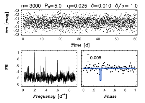
As an introductory example of the power of the BLS algorithm, we show in Fig. 1 the result of the analysis of a test signal with very low signal-to-noise ratio. Here and in all subsequent simulations we assume all data points have the same noise level, characterized by $\sigma$, and therefore the signal-to-noise ratio (SNR) is defined by $\delta/\sigma$. The figure demonstrates that the BLS spectrum is able to identify the correct period even at a high noise level. Several high peaks appear in the spectrum at integer fractions and multiples of the true period. This feature is common in all methods utilizing higher harmonics of the signal. In this example we used 50 bins, which is a reasonable compromise between computational efficiency and signal resolution (see next section for details). In plotting the folded time series we used 100 bins. Here and in all subsequent figures the full frequency band is divided into $\approx 1000$ bins and only the maxima in these bins are plotted. In this way all important information is retained and showing unnecessary details is avoided. The final spectra are normalized in the $[0,1]$ interval.

3 Properties of the Box-Fitting algorithm

This section focuses on the applicability of the Box-fitting algorithm to different time series, and to give signal- and noise-dependent confidence limits. Due to the statistical complexity, most of the results are based on extended numerical tests. Nevertheless, whenever possible, we also present some analytical approximations.

In all subsequent tests the signals have a period of $5^{d}$ and span a timebase $T$ of $60^{d}$. The signal is sampled at times $t_{i}=(i-1+\vartheta)T/n$, where $\vartheta$ is a uniformly distributed random variable in $[0,1]$. This distribution corresponds to the timings we may obtain during a short but concentrated and continuous observational campaign from several ground-based observatories or from space. If the sampling or test periods are different from the ones used in this paper, the main results presented here still remain valid, assuming that the distribution of the data in the folded time series at any trial period is basically uniform. Our non-periodic sampling yields aliasing-free spectra in the frequency band of interest. We do not deal with aliasing effects originating from nearly periodic sampling, because this problem affects all period searching algorithms in a similar way.

In all our simulations, the search for the fractional transit length is performed in the $[0.01,0.10]$ range. The upper limit is well above the expected maximum fractional transit length for planets (see Defaÿ et al. 2001), but is in the right range for detached binaries.

The frequency spectra are computed in the $(0.02,0.91)d^{-1}$ band, a range that contains frequency components of the true period from the $10^{th}$ subharmonics up to the $3^{rd}$ harmonics. Usually we use 4000 frequency steps, because, due to the specific signal shape, the line profiles are very narrow. Therefore, our algorithm requires a much finer sampling than DFT (see also Stellingwerf 1978).

To characterize the Signal Detection Efficiency we introduce (see also Alcock et al. 2000):

$$SDE = {{SR_{\rm peak}-\langle SR\rangle}\over{sd(SR)}}\hskip 5.69054pt,$$ (6)

where $SR_{\rm peak}$ is the $SR$ at the highest peak, $\langle SR\rangle$ is the average, and $sd(SR)$ is the standard deviation of $SR$ over the frequency band tested. Because in the practical computation of $SDE$ one uses all available spectral points, in the presence of periodic signal, the actual value of $SDE$ also depends on the time spanned by the data and on the lengths and position of the frequency band of the analysis. If all other parameters are kept constant, increasing time span or frequency band leads to an increase in $SDE$ for signals containing periodic component(s). This is because under the condition mentioned, the relative contributions to $\langle SR\rangle$ and $sd(SR)$ of the peaks associated with the signal become smaller. Of course, aliasing leads to a decrease in $SDE$.

3.1 Dependence on the transit phase

In the practical implementation of BLS one has to satisfy two conflicting requirements: (a) a high time resolution — demanding a large number of bins; (b) short execution time and statistical stability — supporting a small number of bins. For example, assuming a fractional transit length of 2%, one would like to have at least 50 bins, otherwise the transit signal will be included in a wider bin, degrading the signal. However, 50 bins in such a case are not enough, because in most cases the transit will be divided into two bins, causing the same effect. For a more secure coverage we would probably need to double or triple the number of bins. However, this could be rather time consuming, especially if the allowed range of fractional transit length is assumed to be large (say $>0.1$). The sensitive dependence of the execution time on the number of bins follows from the fact that the number of operations in the BLS algorithm is proportional to $m(\Delta i_{max}-\Delta i_{min})$, and $\Delta i_{max}-\Delta i_{min}\sim m(r_{max}-r_{min})$.

Figure 2: BLS spectra computed for two different transit phases for the same number of bins and signal parameters, shown in the header.

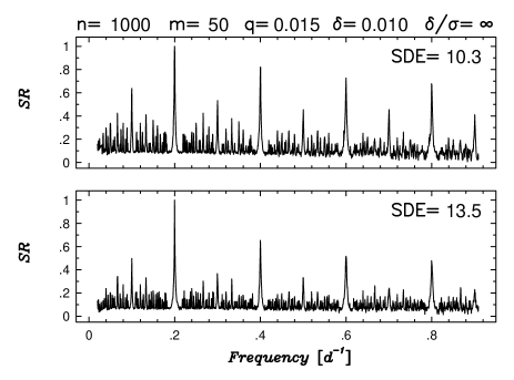
When using a finite bin size, we expect some dependence of the BLS spectra on the transit phase, i.e., on the position of the transit within the folded time series. We illustrate this effect in the case of a noiseless signal in Fig. 2. The figure shows the strong increase of the power in the harmonic and subharmonic components, in addition to similar changes in other substructures of the frequency spectrum.

Figure 3: Dependence of the $SDE$ of the BLS spectra on the transit phase for noiseless signals with parameters shown in the header.

Figure 4: As in Fig. 3, but for a signals of shorter fractional transit length.

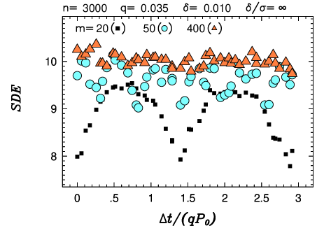
In order to have a better idea of the possible ranges of $SDE$ for different numbers of bins, we show in Fig. 3 the $SDE$ as a function of the fractional transit phase $\Delta t/(qP_{0})$, where $\Delta t$ denotes the shift in time of the starting moment of the transit with respect to some arbitrary epoch. The transit length is chosen so that at $m=50$ the bin size is about half the transit length. The figure shows that even this number of bins displays relatively large variations of $SDE$ as a function of the transit phase, let alone the $m=20$ case. The high number of bins clearly yields high, more stable $SDE$. However, the necessary increase in the CPU time is rather high (see later). On the other hand, the low number of bins may yield a fairly low $SDE$, due to occasional partial coverage of the transit and wide bin size. The periodicities in $SDE$ come from the equidistant bin distribution and are given by $(mq)^{-1}$ in units of $qP_{0}$.

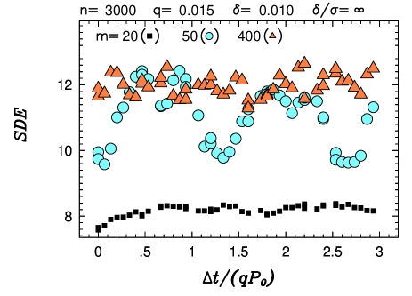
The $SDE$ dependence on the transit phase is a function of the transit length. To show this function we plot in Fig. 4 the same dependence for a transit length of $q=0.015$, instead of $0.035$ as in Fig. 3. We see now that the $SDE$ corresponding to $m=20$ is stable, although with lower values. This is so because for a small number of bins the full transit is included in one bin in most cases — yielding $SR$ values independent of the transit phase. The strong dependence on the transit phase occurs when the bin size is comparable to the actual length of the transit. In both examples, a high enough number of bins yields higher, and more stable $SDE$, which, in the presence of noise, means also a higher probability of signal detection (see Sect. 3.3).

3.2 Response to pure noise

One of the most important features of any search algorithm is its ability to distinguish between false and true signals. In our case, this translates to the estimation of the statistical significance of the highest peak in the BLS spectrum. To study this question we performed intensive numerical tests to derive the Probability Distribution Function (PDF) of $SDE$ in case the input data contain only Gaussian noise.

Figure 5: Probability distribution functions of $SDE$ for the BLS method at various numbers of test frequencies shown at the horizontal lines. Thick lines are for the empirical (numerical), thin lines are for the semi-theoretical results described in the text.

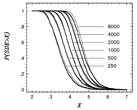
Our results show that the PDFs depend only on the number of trial frequencies $n_{f}$, and are immune (within the numerical stability of the simulations) to changing the number of data points or number of bins used by the BLS algorithm. In order to ensure reasonable numerical stability, we use in all cases 1500 realizations to estimate the corresponding PDF. The number of data points is set to 500, 1000, or 2000, while the number of bins is chosen to be 50 or 100. Fig. 5 displays the empirical PDFs obtained for various numbers of trial frequencies.

One could expect the probability of finding outstanding peaks in a noisy spectrum to increase with the number of sampled frequencies, if the samples were statistically independent. We derive a theoretical PDF by using this assumption, and show that adjustment of this PDF to the empirical one is possible, with parameters different from the ones predicted by the assumption of large independent samples.

The computation of $SDE$ consists of two major steps: (a) selection of the largest $SR(i_{1},i_{2})$ at each trial period, (b) selection of $SR_{\rm peak}$ — the largest $SR$ of all the values computed for the $n_{f}$ trial frequencies. In general we have $mn_{f}\gg n$, and therefore it is obvious that many of the tested $SR(i_{1},i_{2})$ values cannot be considered to be independent samples. Therefore, in this — admittedly not exact, but, as we shall show below, quite practical — approach, it is assumed that the distribution of $SDE$ can be approximated by the one obtained for $\tilde{n}$ independent samples of $SR(i_{1},i_{2})$, where $\tilde{n}$ is to be determined by numerical simulations.

Assume, for the sake of simplicity, that all data points have the same error, $\sigma$. We take $\tilde{n}$ independent values of the random variable $SR(i_{1},i_{2})$, identify the highest value $SR_{\rm peak}$ and compute $SDE$. For a large sample size we can assume the values of $\langle SR\rangle$ and $sd(SR)$ are constant. Therefore, one can use Eq. (6) to write the probability that $SDE$ exceeds a specified value $X$:

$$P(SDE>X) = P(SR_{\rm peak}>x)\hskip 5.69054pt,$$

where $x=X\times sd(SR)+\langle SR\rangle$. Let $p$ be the probability that a given sample of $SR$ has a value larger than $x$. Then,

$$P(SDE>X)=P(SR_{\rm peak}>x)=1-(1-p)^{\tilde{n}}.$$

The value of $p$ can be calculated under the assumption of pure noise. In such a case $SR$ is actually the absolute value of a zero-mean Gaussian random variable with a variance of $\sigma^{2}/n$. This distribution implies $sd(SR)=a\sigma/\sqrt{n}$ and $\langle SR\rangle=b\sigma/\sqrt{n}$ where $a=\sqrt{1-2/\pi}=0.60$ and $b=\sqrt{2/\pi}=0.80$. To facilitate the calculation of $p$ we can use the normalized random variable $\chi=SR\sqrt{n}/\sigma$ and write:

$$p = P(SR>x)$$ (7)

$$= P(\chi>x\sqrt{n}/\sigma)$$

$$= 2(1-\Phi(x\sqrt{n}/\sigma))$$

$$= 2(1-\Phi(aX+b))\hskip 5.69054pt,$$

where $\Phi$ is the commulative distribution function of the normalized Gaussian variable. If all the $n_{f}$ samples were independent, we could use $n_{f}$ instead of $\tilde{n}$. Since this is not the case, in order to generalize the above calculation we assume that the effective $\tilde{n}$ is related to $n_{f}$ by some power law: $\tilde{n}=n_{f}^{c}$. The parameters $a$ and $b$ depend on the assumption of constant standard deviation and mean of $SR$ as well as on its specific distribution. Therefore, in order to fit the empirical PDFs we allow the three parameters $a$, $b$ and $c$ to vary. The best-fit values we get are: $a=0.67$, $b=0.36$, $c=0.83$. These values are significantly different from the ones obtained with our simplifying assumptions. However, as Fig. 5 shows, the functional form of the above PDF with the fitted parameters gives a good approximation of the numerical results.

3.3 Signal detection power

Before turning to the numerical simulations, we derive a simple estimate of the minimum number of data points necessary obtain a high enough signal detection probability. Here we deal with the folded time series at the signal period, and ask the question whether the differences in $SR^{2}(i_{1},i_{2})\equiv s^{2}(i_{1},i_{2})/[r(i_{1},i_{2})(1-r(i_{1},i_{2}))]$ between the values including or excluding the transit event are significant. We therefore evaluate the Dip Detection Efficiency:

$$DDE = {{E[SR^{2}(j_{1},j_{2})]-E[SR^{2}(k_{1},k_{2})]}\over\sqrt{\sigma^{2}[SR^{2}(j_{1},j_{2})]+\sigma^{2}[SR^{2}(k_{1},k_{2})]}}\hskip 5.69054pt,$$ (8)

where the indices $j$, $k$ refer to the ‘in’ and ‘out’ of transit values, respectively, and $E[...]$, $\sigma^{2}[...]$ stand for the expectation value and variance of the corresponding random variable. If we assume equal noise for all data points and optimal bin size (i.e., $r=q$), then the averages and standard deviations read:

$$E[SR^{2}(i_{1},i_{2})] = S_{0}+{\sigma^{2}\over{n}}\hskip 5.69054pt,$$

$$\sigma^{2}[SR^{2}(i_{1},i_{2})] = 4S_{0}{\sigma^{2}\over{n}}+2{\sigma^{4}\over{n^{2}}}\hskip 5.69054pt,$$ (9)

where $S_{0}$ denotes the corresponding noise-free value of $SR^{2}(i_{1},i_{2})$, with $i=j$, $S_{0}=q(1-q)\delta^{2}$ for the ‘in transit’ and $i=k$, $S_{0}=\delta^{2}q^{3}/(1-q)$ for the ‘out of transit’ cases. By employing the $q\ll 1$ condition and retaining only the leading terms in $q$, and omitting the quartic terms in $\sigma$, it is easy to get the final expression for $DDE$

$$DDE = {1\over 2}{\delta\over\sigma}\sqrt{nq}\hskip 5.69054pt.$$ (10)

Based on this result, we use

$$\alpha\equiv{\delta\over\sigma}\sqrt{nq}$$ (11)

to parameterize the effective SNR, because $\sigma/\sqrt{nq}$ is the standard deviation of the average of all measurements within the transit.

Figure 6: Signal detection efficiency for noisy signals as a function of $\alpha\equiv{\delta\over\sigma}\sqrt{nq}$. The same bin number of $100$ and fractional transit length of $0.033$ are used in all simulations.

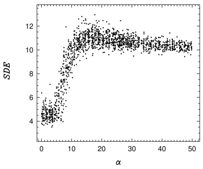
We performed $1500$ simulations with $m=100$, $\delta=0.01$, $q=0.033$, $n=1000$–$4000$, and various transit phases. The dependence of $SDE$ on $\alpha$ is shown in Fig. 6. We see that at $\alpha<5$ the $SDE$ values are noise-dominated at about constant level, almost exclusively below 6. The $SDE$ values generated by pure noise fall also under $6$ with very high probability (see Fig. 5). In the range of $\alpha=6-13$, $SDE$ displays a sharp linear increase, until it reaches a mild maximum. It turns out that when $\alpha$ gets to the linear increase region, the associated value of $SDE$ starts to become significant.

Figure 7: Differential signal detection efficiency for noisy signals as a function of $\alpha$. Shaded circles and filled squares show results for $\Delta(SDE)=SDE_{m=200}-SDE_{m=20}$, and $SDE_{m=50}-SDE_{m=20}$, respectively. The transit length is the same in all cases and is chosen to be relatively small, i.e., $q=0.015$.

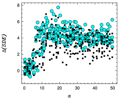
Tests performed with other numbers of bins show that the above pattern remains the same, with the sole difference that for a larger number of bins $SDE$ reaches larger maxima, and therefore, the linear region between $\alpha=6$ and $13$ becomes steeper. It is important to note that the region of $\alpha$ around 6 is critical in all cases, because of the separation between the stochastic and deterministic signal detections. As we could expect, this regime coincides with the $\approx 3\sigma$ limit of $DDE$ (see Eq. (10)).

In the above simulations we fixed the fractional transit length at a relatively large value, in order to ensure reasonable resolution with $100$ bins. With a shorter transit length, at the same number of bins, the $\alpha>15$ region becomes fuzzier, with a somewhat higher average value of $SDE$ (at least for moderately smaller transit lengths). However, the global properties remain the same as described above.

The response of $SDE$ to changing the number of bins is illustrated in Fig. 7. We see that a substantial increase of $SDE$ can be gained in many cases by moving from 50 bins to 200 bins. Of course, for longer transit lengths, the gain is smaller.

4 Comparison with other methods

The purpose of this section is to illustrate that the method introduced in this paper enables us to discover periodic transit-type events in noisy time series with a (much) higher probability than the other standard period searching algorithms available in the current astronomical literature. In all subsequent examples we use $m=200$ for the BLS method.

Figure 8: As in Fig. 6, but for the W-R method with $100$ bins.

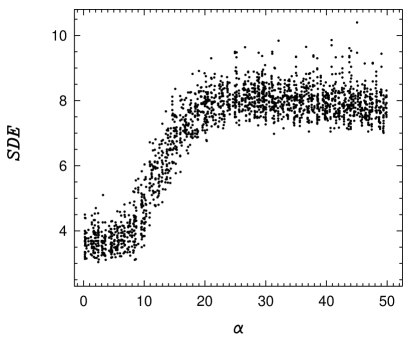
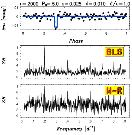
Perhaps the most competitive method is that of W-R (or similarly, PDM of Stellingwerf 1978). Therefore, we perform the same test for this method as the one presented in Fig. 6 for the BLS method. The result is shown in Fig. 8. For compatibility, we use the same bin number and signal parameters as for the simulations shown in Fig. 6. In comparison, we see that the W-R method yields a wider transition region between the noise- and signal-dominated regimes. Furthermore, the value of $SDE$ is lower in the signal-dominated region. In order to illustrate the appearance of these differences in the frequency spectra, we show a representative example in Fig. 9. We use $100$ bins in the W-R method, because a larger number leads to an even poorer performance of this method.

Figure 9: Comparison of the BLS and W-R methods for a realization of a signal with parameters shown in the header (other parameters are standard, as given in Sect. 3). The uppermost panel shows the folded/binned time series (dots) with the period and the fit (continuous line) obtained by the BLS method.

The next example examines the L-K method. We recall that in this method the squared differences between the bin-averages are computed for each folded time series. For large bin numbers and smoothly varying time series, this method should yield very small (in the limiting case, zero) L-K statistics at the correct period.

Figure 10: As in Fig. 9, but for the L-K method. On the ordinate axis for the L-K method, $SD$ stands for ‘standard deviation’, the corresponding statistics of the L-K method. Minima of $SD$ indicate periodicities in the signal by the the L-K statistics.

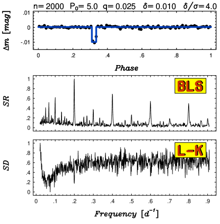
Certainly, in the case of periodic signals with discontinuous variations, such as the ones studied in this paper, the L-K method should give non-zero statistics even in the noiseless case. Indeed, even for very high SNR, the L-K method performs extremely poorly (see Fig. 10). We use $500$ bins for the L-K method, because tests have shown that at lower values the L-K method performs even more poorly. By decreasing SNR to 2-3, there remains no significant dip close to the test frequency (or to its harmonics) in the L-K spectrum. It is important to recall that this noise level still corresponds to $\alpha=14$–$21$, well above the secure signal detection limit for BLS.

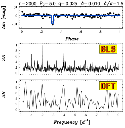
As expected, DFT is also not preferable for analyzing signals with periodic transits of short duration. In the noiseless case, DFT yields very slowly decreasing power for the successive harmonics. Although this is not a good property for correct period identification, DFT shows a reasonable stability against noise. As shown in Fig. 11, some remnant power at (or close to) the original harmonics is still visible in the DFT spectrum, but a reliable identification is not possible even at this high SNR ($\alpha=11$). At an even higher SNR, corresponding to $\alpha=14$, the main component becomes the highest amplitude peak, with a simultaneous increase of the harmonics and with a still considerable contribution from other parts of the spectrum, originating from the noise.

Figure 11: As in Fig. 9, but for the DFT method.

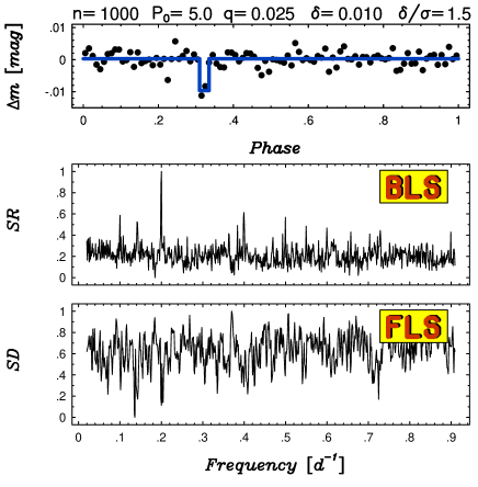
Finally, one can attempt to use multifrequency LS Fourier fit (FLS) for better approximation of the signal shape and thereby increasing the $SDE$ in the case of the Fourier method. (We note that for data distribution leading to orthogonal Fourier base, the method of Defaÿ et al. (2001) is equivalent to this direct LS Fourier approach.) Because of the substantial increase in execution time for this method, we use a smaller number of data points and limit the order of the Fourier fit to $10$. By plotting the standard deviation of the residuals, we obtain the result shown in Fig. 12. Although the performance of FLS could be improved by using more harmonics, FLS did, in general, a considerably poorer job at moderately high noise levels (similarly to the one shown in Fig. 12).

Figure 12: As in Fig. 9, but for the the Fourier-sum-fitting Least Squares method with 10 components. Minima in the FLS spectrum indicate periodicities in the signal.

Computational efficiency of the BLS method has been tested in comparison with DFT on a sun workstation. For proper comparison, the same data sets and the same number of frequency steps were computed by both methods, although DFT requires about an order of magnitude fewer steps, because of its wider line profiles. The range of the search for the best fractional transit length in the BLS method was fixed at $[0.01,0.10]$, as mentioned at the beginning of Sect. 3. Table 1 shows that, except for high bin numbers and low number of data points, BLS surpasses DFT in execution time per frequency step. While the CPU time required by DFT is determined by the number of data points, BLS depends much less on this parameter. The BLS execution time can be decreased by decreasing the allowed range of fractional transit length. For example, with $n=8000$, $m=500$ the execution time decreases to $13$ s, if $[r_{\rm min},r_{\rm max}]=[0.005,0.03]$. Note that by increasing the $SDE$ of the Fourier method with the aid of a multifrequency least squares approach (or its nearly equivalent version using sum of the amplitudes of the harmonics — see Defaÿ et al. 2001) the execution time will increase substantially (proportional to the number of harmonics) for the Fourier method. A multifrequency Fourier method must use frequency steps as small as for the BLS method, while it has to use at least $7$–$10$ harmonics to approximate reasonably closely the $SDE$ of the BLS method. We therefore suggest that the BLS method can be considered a very efficient tool to analyze transit-type signals.

Table 1: Comparison of the execution times

n	m	$t_{\rm BLS}[sec]$	$t_{\rm DFT}/t_{\rm BLS}$
1000	50	1.0	6.5
	100	1.6	4.1
	200	4.0	1.6
	500	19.1	0.3
5000	50	4.3	7.6
	100	5.0	6.6
	200	7.6	4.3
	500	22.6	1.5
8000	500	25.0	2.1

Notes: $-$ 5000 test frequencies are computed
           $-$ a sun Ultra 300 MHz machine is used with
               an optimized fortran compiler

5 Conclusions

This paper has examined the statistical characteristics of the Box-fitting Least Squares algorithm to detect periodic transits in time series of stellar photometric observations. The algorithm strongly relies on the anticipated box-shape of the periodic light curve. The advantage of using a predetermined shape of the light curve manifests itself in the high efficiency of this method relative to the other search methods, which are generic and can detect any periodic variation.

The algorithm studied here assumes only two levels of the periodic light curve. This assumption ignores all other features that are expected to appear in planetary transits. Thus, we ignore the gradual ingress and egress phases of the transit, which carry important information about the parameters of the planetary orbit (e.g, Sackett 1999). The lengths of these phases are short compared to the transit and thus they are not expected to affect significantly the results of the search. Another effect we ignore is the limb-darkening effect, which has indeed been shown to be small in the case of HD 209458 (e.g., Deeg et al. 2001). The effectiveness of the algorithm relies on the above simplifying assumption, which is justified as long as we are interested in a detection tool. After the periodicity is detected we can try to recover subtle features of the folded light curve, in order to derive the stellar and the planetary characteristics.

Our main interest is in cases where the signal-to-noise ratio is small, and one cannot identify the signal by monitoring a single transit, because the stellar drop in intensity is buried in the noise. Contrary to the search of transits by the HST in 47 Tuc (Gilliland et al. 2000), where the noise was small relative to the expected transit dip, we concentrate on cases in which the periodic signal can be detected only after many measurements are accumulated and the unknown transit is monitored many times. To be able to deal with a large number of observations, of a thousand or more, we have introduced binning into the folded data. We have shown that as long as the bin size is small compared to the expected transit length, the efficiency of the method is not affected.

One additional factor that determines the computational load of the algorithm is the range of transit length searched for. The maximum possible transit length can be estimated if we know the orbital, stellar and planetary radii. For a given stellar mass, the stellar radius can be derived by the mass-radius relation, and the orbital radius can be derived for any period. Recent theories give some estimates for the planetary radii. Therefore, for a given stellar mass we can estimate the maximum duration of the transit, which for HD 209456 is only a few percent of the period. For most ground-based and space searches for planetary transits one would have some idea of the stellar mass of all transit candidates, and therefore we can make our algorithm computationally more efficient by imposing a variable maximum duration on the transit length.

The significance of the detection depends primarily on the effective signal-to-noise ratio of the transit. The signal is the stellar brightness within the transit, relative to the brightness outside the transit, and the noise is the expected scatter of the measured average of the stellar brightness inside the transit. The scatter is composed, obviously, of the observational noise as well as of stochastic variation of the stellar intensity. It seems that the effective signal-to-noise ratio should exceed $6$ in order to get a significant detection. This requirement should be taken into account when planning future searches for extrasolar planetary transits.