Measuring starspots on magnetically active stars with the VLTI

Abstract

We present feasibility studies to directly image stellar surface features, which are caused by magnetic activity, with the Very Large Telescope Interferometer (VLTI). We concentrate on late type magnetically active stars, for which the distribution of starspots on the surface has been inferred from photometric and spectroscopic imaging analysis. The study of the surface spot evolution during consecutive rotation cycles will allow first direct measurements (apart from the Sun) of differential rotation which is the central ingredient of magnetic dynamo processes. The VLTI will provide baselines of up to 200 m, and two scientific instruments for interferometric studies at near- and mid-infrared wavelengths. Imaging capabilities will be made possible by closure-phase techniques. We conclude that a realistically modeled cool surface spot can be detected on stars with angular diameters exceeding $\sim$ 2 mas using the VLTI with the first generation instrument AMBER. The spot parameters can then be derived with reasonable accuracy. We discuss that the lack of knowledge of magnetically active stars of the required angular size, especially in the southern hemisphere, is a current limitation for VLTI observations of these surface features.

Markus Wittkowski, mwittkow@eso.org

1 Introduction

Optical interferometers are about to become powerful instruments to image vertical and horizontal temperature profiles and inhomogeneities of stellar surfaces. Direct observations of these structures will be the key for constraining underlying hydrodynamic and magneto-hydrodynamic mechanisms and for our further understanding of related phenomena like predictions of stellar activity and asymmetric or stochastic mass-loss events. The study of the evolution of surface spots which are caused by magnetic activity, during consecutive rotation cycles will allow first direct measurements (apart from the Sun) of differential rotation which is the central ingredient of magnetic dynamo processes.

Many starspots have been discovered by photometric monitoring (e.g. Strassmeier et al. 1999). The distribution of starspots on the surfaces of stars has so far been inferred from photometric and spectroscopic imaging analysis for about 50 stars (”Summary of Doppler images of stars”, www.aip.de/groups/activity/DI/summary). In addition, there is evidence for surface features on some slowly rotating single K giant stars based on Ca II variability (e.g. Choi et al. 1995). The observation of these stars may not be very feasible for Doppler imaging techniques because of their slow rotation. However, they might be good candidates for interferometric imaging, here because of their slow rotation, and their sufficiently large angular diameters (Hatzes et al. 1997). Magnetic activity is usually assumed to be the cause for these surface spots.

Optical interferometry has already proven its ability to derive stellar surface structure parameters beyond diameters. The limb-darkening effect on stellar disks was confirmed by interferometry for several stars by Hanbury Brown et al. (1974), Haniff et al. (1995), Quirrenbach et al. (1996), Burns et al. (1997), Hajian et al. (1998), Young et al. (2000), and Wittkowski et al. (2001). The latter measurement did not only succeed in discriminating uniform disks and limb-darkened disks, but also in constraining model atmosphere parameters. For the apparently largest supergiants $\alpha$ Orionis, $\alpha$ Scorpii and $\alpha$ Herculi, bright spots have been detected and mapped by direct imaging techniques including optical interferometry and HST imaging (Buscher et al. 1990, Wilson et al. 1992, Gilliland & Dupree 1996, Burns et al. 1997, Tuthill et al. 1997, Young et al. 2000). Large-scale photospheric convection (Schwarzschild 1975, Freytag et al. 1997) is a preferred interpretation for the surface features on the these supergiants, and for interferometric observations of asymmetric features on or near stellar disks (see, e.g. Perrin et al. 1999, Weigelt et al. 2000) or circumstellar envelopes (see, e.g. Weigelt et al. 1998, Wittkowski et al. 1998).

The ESO VLTI (Very Large Telescope Interferometer), a European general user interferometer located on Cerro Paranal in northern Chile, is about to become an excellent facility to study stellar surfaces by means of optical interferometry. It will provide a large choice of baselines up to 200 m, the use of the 8 m Unit Telescopes (maximum baseline 130 m), of several 1.8 m Auxiliary Telescopes as well as of a near-infrared instrument (AMBER, see Petrov et al. 2000), and a mid-infrared instrument (MIDI, see Leinert et al. 2000). The AMBER instrument will provide imaging capabilities by closure-phase techniques. For a description of the VLTI and the recent achievement of first fringes see Glindemann et al. (2000), Glindemann et al. (2001a), Glindemann et al. (2001b), and references therein. Since then, commissioning activities have been carried out. VLTI commissioning data of scientific relevance are being publicly released (www.eso.org/projects/vlti/instru/vinci/vinci_data_sets.html). Measurements of visibility amplitudes beyond the first minimum of the visibility function, which is mandatory for an analysis of stellar surface features, became already feasible with the commissioning instrument VINCI (see ESO Press Release 23/01; Wittkowski et al., in preparation). The potential to study stellar surfaces with the VLTI has previously been investigated by von der Lühe et al. (1996), Hatzes (1997) and von der Lühe (1997). Other existing or planned ground-based optical and near-infrared interferometric imaging facilities (with location and maximum baseline) include the CHARA (Mt. Wilson, USA, 350 m), COAST (Cambridge, UK, 100 m), IOTA (Mt. Hopkins, USA, 40 m), NPOI (Flagstaff, USA, 437 m), KECK (M. Kea, USA, 140 m), LBT (Mt. Graham, USA, 22 m), OHANA (M. Kea, USA, 800 m). In addition, free-flying space-based interferometers are being designed. For instance, the “stellar imager” (SI), a NASA design for a space-based UV/optical interferometer with a characteristic spatial resolution of 0.1 mas, is especially intended to image dynamo activity of nearby stars (hires.gsfc.nasa.gov/ si).

Here, we investigate to which extent and accuracy surface features with realistically modeled parameters can be analyzed in the near future by VLTI measurements using first generation instruments. Observing restrictions and accuracy limits are taken into account. We concentrate on magnetically active stars and studies which aim at understanding stellar magnetic dynamo processes.

2 Potential sources

The VLTI with its first generation instruments will provide a maximum baseline $B$ of 200 m and a shortest wavelength $\lambda$ of 1.0 $\mu$m using the AMBER instrument at the lower end of its wavelength range. With this instrument, one resolution element $\lambda/B$ will correspond to an angular size of 1.0 mas. Requiring at least two resolution elements across the stellar disk, the minimum diameter is about 2.0 mas. The use of the longest (200 m) VLTI baseline implies that the 1.8 m Auxiliary Telescopes are employed, and the anticipated limiting J magnitude is about 6 mag, assuming that fringes are tracked on a shorter baseline (baseline bootstrapping).

However, despite these limitations for the use of the VLTI, other ground-based optical interferometers, as for instance the completed NPOI with a characteristic maximum resolution of $\sim$ 0.3 mas, or even planned space-based UV interferometers (e.g. SI), will be able to image smaller bright stars. Consequently, the search for potential sources, i.e. for stars which are known to exhibit spots, was not restricted due to diameters. Stellar diameters were estimated for stars which are known or expected to have spots on their surface. The resulting full table is described and shown in Appendix A. This list serves as source of information on potential targets for interferometric imaging. Depending on the location and characteristics (e.g. baseline, observing wavelengths, limiting magnitude) of an interferometer, certain restrictions apply to the choice of feasible targets from the lists in Appendix A. Restrictions due to the array geometry like shadowing effects or limited availability of delay line lengths might arise in addition. Further limitations on the amount of observational data that can be combined for the purpose of imaging techniques may apply due to the rotational velocity of the star.

Most stars on the lists in Appendix A belong to one of the following classes of objects: RS CVn type, BY Dra type, W UMa type, FK Com type, T Tau type and single giants. Single giants are in principle good candidates for interferometric imaging, because they are relatively large and usually they rotate slowly. In addition, observations are not affected by companions in the field of view. However, most single giants are not expected to be magnetically active and information on parameters of spots caused by magnetic activity is rare. Doppler images have so far been obtained for only one magnetically active effectively single giant, namely HD 51066 or CM Cam (Strassmeier et al. 1998). HD 27536 is another example of this rare class and has been discovered by photometric monitoring (Strassmeier et al. 1999b). Other single giants are suspected to be magnetically active and to harbor spots on their surfaces, based on Ca II variability (Choi et al. 1995).

Table 1: Stars with known surface spots from the Tables in the Appendix which are feasible for VLTI observations with AMBER, i.e which have an estimated diameter of larger than 2 mas, a declination of less than 30 degrees, and a J magnitude of brighter than 6. Shown are the star’s name, variability type, declination, rotation period, and diameter. The diameter is the mean of measured diameters, if available, or the mean of estimated diameters. The last column indicates whether or not Doppler images are available.

Name	Type	Dec.	P	$\theta$	Doppler
		(deg)	(d)	(mas)	images
$\zeta$ And	RS CVn	+24	17.6	2.8	no
$\sigma$ Gem	RS CVn	+28	19.5	2.4	yes
$\Theta^{1}$ Tau	giant	+16		2.6	no
$\gamma$ Com	giant	+28		2.5	no

Table 1 shows four stars from the lists in Appendix A which are feasible for VLTI observations. They include two RS CVn type variables and two single giants. The rotational periods of the RS CVn type stars $\zeta$ And and $\sigma$ Gem of 17.6 days and 19.5 days, respectively, allow observations during 6 hours with a smearing effect of only about 5 degrees. However, the existence of the companion stars may lead to effects which complicate the interpretation of the visibility data. Doppler images exist for the RS CVn type giant $\sigma$ Gem, providing us with characteristics on the spots.

The objects listed in the Appendix A have mostly been observed in the northern hemisphere. It would be desirable to initiate similar photometric and spectroscopic variability studies in the southern hemisphere which could serve as a preparation and source of complementary information for VLTI measurements of stellar surfaces.

3 Interferometric imaging

The observables of an interferometer are the amplitude and phase of the complex visibility function, which is the Fourier transform of the object intensity distribution. In presence of atmospheric turbulence, usually only the squared visibility amplitudes and the triple products are accessible by optical and near-infrared interferometers. The triple product is the product of three complex visibilities corresponding to baselines that form a triangle. The phase of the triple product, the closure phase, is free of atmospheric phase noise (Jennison 1958). An image can usually only be reconstructed if at least three array elements are used simultaneously. The general methods to reconstruct an image from sparse aperture interferometric visibility data have been developed by radio astronomers. In fact, the first images (Baldwin et al. 1996, Benson et al. 1997, Hummel et al. 1998) that were reconstructed from optical interferometric data using the COAST and NPOI interferometers employed imaging software which is usually used by radio interferometrists. As an example for interferometric imaging of starspots, Hummel (1999) showed by simulated NPOI data that a star with one spot (stellar diameter 12 mas, spot diameter 3 mas, $T_{\mathrm{star}}=5000$ K, $T_{\mathrm{spot}}=3500$ K) can be imaged by NPOI. A recent review describing the image fidelity using optical interferometers can be found in Baldwin & Haniff (2002).

In order to reconstruct an image of reasonable fidelity, it is intuitively understandable that the number of visibility data has to be at least as large as the number of unknown variables, i.e. the pixel values of the image (see, e.g. Baldwin & Haniff 2002). Furthermore, despite of the ability of imaging algorithms to effectively interpolate the sparse aperture data, the aperture has to be filled as evenly as possible. In case of highly unevenly filled apertures, the point spread function would show strong artifacts (sidelobes) which could not be deconvolved. This implies that most probes of the visibility function have to be taken at points beyond its first minimum. Here, the visibility amplitude is very low, corresponding to vanishing fringe contrasts. This makes it difficult to detect and track the fringes. As a solution, these low fringe contrasts can be recorded while fringes are tracked on shorter baselines with higher contrasts using bootstrapping techniques (see, e.g. Roddier 1988, Armstrong et al. 1998, Hajian et al. 1998, Wittkowski et al. 2001).

The VLTI with the AMBER instrument allows the simultaneous combination of three beams. The maximum feasible size of an image of a stellar disk is limited by the number of visibility data, which can be combined, to less than about 10 $\times$ 10 pixels. For the stars in Tab. 1, which have diameters of only $\sim$ 2.5 mas, the image size is limited to only 2 $\times$ 2 pixels due to the minimum size of one resolution element of 1.0 mas.

Model fitting will often be a better choice than imaging, especially if the feasible size of the image is limited to a few pixels. The use of phase information, i.e measurements of triple products, is mandatory for asymmetric objects. Recent data from the COAST interferometer on Betelgeuse, a star exhibiting surface spots, were in fact analyzed by model fits (Young et al. 2000). A model example of the influence of a stellar surface spot on visibility amplitude, triple amplitude, and closure phase data of a cool giant can be found in Wittkowski et al. (2001).

4 VLTI Simulations

It was discussed in Sect. 2 that single giants are good candidates for interferometric imaging. As a result, the slowly rotating G9 giant $\Theta^{1}$ Tau was chosen from Tab. 1 as a model star for VLTI simulations. With a measured diameter of 2.6 mas (White & Feierman 1987) – which is in good agreement with diameter estimates – it is one of the apparently largest stars for which surface features by magnetic activity have been predicted. It is located at a declination of +16^∘, which is easily reachable from the VLTI at Cerro Paranal (latitude -24^∘ 40’). Its effective temperature was estimated to be 5000 K (Choi et al. 1995). A surface gravity of $\log g=3$ is assumed based on empirical calibrations.

While surface activity is predicted for $\Theta^{1}$ Tau, the characteristics of its surface features are unknown. As a solution, typical spot parameters were assumed for our model star. They were taken from Doppler imaging results of a similar star, the effectively single G8 giant CM Cam (see Sect. 2). The two stars differ in their rotational velocity (period of CM Cam: 16 days, period of $\Theta^{1}$ Tau: 140 days), which may lead to a different level of expected surface activity. Presently, CM Cam as a single giant of about the same spectral type is the best match of a giant for which information on spot parameters exists. Our model describes a CM Cam like star at a for VLTI accessible location on the sky with a more convenient distance, i.e. angular diameter.

Cool spots with an average temperature difference with respect to the unspotted photosphere of $\Delta T=500\pm 300$ K have been found on the surface of CM Cam, as well as a weaker equatorial belt of surface features (Strassmeier et al. 1998). The latter are rather complex features than well defined spots, and hence difficult structures for interferometric imaging. The biggest of the polar spots has been used for our model. It shows a temperature difference of $\Delta T=500\pm 300$ K, and was found at a latitude of +65^∘, with a radius of 15.3^∘ (Strassmeier et al. 1998).

Model

Table 2: Model assumptions. Some parameters are redundant and given for reasons of clarity only. The parameters which are directly used for our model are marked by italic font.

Parameter	Value
Observing wavelength	1.0 $\mu$m
Declination	+16∘
Stellar rotation period	140 days / 16 days
Inclination of rotation axis	60∘
Stellar diameter	2.6 mas
Stellar effective temperature	5000 K
Stellar surface gravity	$\log g=3$
Metallicity	Solar
Limb darkening parameter $\alpha$ for $I=\mu^{\alpha}$	0.33
Spot diameter	0.5 mas
Spot separation from the stellar center	0.7 mas
Position angle of the spot	90∘
Spot temperature	4500 K
Ratio of spot flux to that at unspotted area	0.71
Rel. offset intensity of the spot	-0.01

Figure 1: Illustration of our model star. Shown are the image (top), the visibility amplitude (middle), and the visibility phase (bottom) of our model star (right), compared to the same star without a surface spot (left). Model parameters were used as given in Tab. 2. The $\times$-symbol on the image of the model star denotes the position of the stellar pole. Visibility amplitude values $\in[0,0.2]$ are shown in logarithmic scale. The spatial frequency range for the visibility amplitudes and phases is $[-2000,2000]$ cycles/arcsec, corresponding to an angular resolution of up to 0.5 mas, i.e. up to a projected baseline of 400 m at a wavelength of 1 $\mu$m. The VLTI with a maximum baseline of $\sim$ 200 m operating at a wavelength of 1 $\mu$m can use half of the range shown here. As another example, the NPOI with a maximum baseline of 437 m operating at a wavelength of about 750 nm can use $\sim$ 1.5 times the shown range for bright stars. Horizontal and vertical cuts through the different panels are shown in Fig. 2.

Figure 2: Horizontal (left) and vertical (right) cuts through the different panels of Fig. 1, i.e. through the model images (top), visibility amplitudes (middle), and visibility phases (bottom). The solid lines denote our used model star, and the dotted lines the same star without a surface spot.

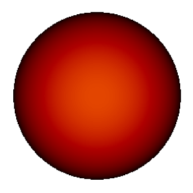
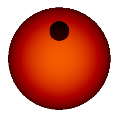
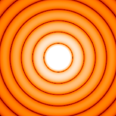
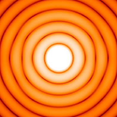
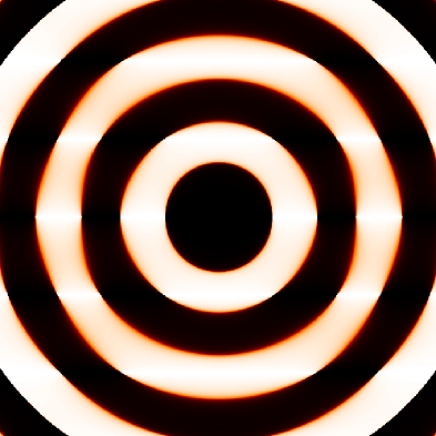
A model star is considered with parameters based on the characteristics of $\Theta^{1}$ Tau for the star parameters and CM Cam for the spot parameters. The model parameters are listed in Table 2. The stellar intensity function $I$ is described by a limb-darkened disk $I=\mu^{\alpha}$ with $\mu=\cos\theta$ being the cosine of the angle between the line of sight and the normal of the surface element of the star, and $\alpha$ a positive real number (see Hestroffer 1997). The parameter $\alpha$ was determined so that the integral of the normalized intensity function is the same as that of the tabulated intensity values of the corresponding Kurucz model atmosphere (Kurucz 1993). Figure 1 shows an image of our model star, as well as the visibility amplitude and visibility phase of this image, compared to an unspotted star. Figure 2 shows horizontal and vertical cuts through the different panels in Fig. 1.

Accuracy of the AMBER instrument

The anticipated accuracy of the AMBER instrument is given as follows. The numbers in brackets denote the goals. Contrast stability 10^-2 in 5 min (10^-3). Visibility accuracy 1% at 3 $\sigma$ (0.01% at 1 $\sigma$). Differential phase stability 10^-2 rd in 1 min (10^-4 rd). The horizontal cuts through the visibility amplitudes in Fig. 2 show a relative difference between the two models, i.e. the spotted star and the unspotted star, of $\sim$7% at the maximum of the second lobe. This difference is significant with an accuracy of 1% at the 3 $\sigma$ level as given for the AMBER instrument. Additional calibration errors are expected to be $\sim$ 1%, based on the anticipated contrast stability. As a result, it can be expected that the given differences can well be detected. However, similar differences at this point of the visibility function are for example expected for a stellar disk with different limb-darkening parameter. Hence, measurements at different evenly distributed points of the $uv$-plane have to be performed in order to unambiguously detect a surface spot (see discussion in Sect. 3). For instance, a stellar disk without a surface feature will not lead to the flip of the two model visibility amplitudes between the second and fourth lobe. In addition, deviations of the visibility phase from values zero and $\pi$ are an unambiguous signature of asymmetric structures and, hence, an essential indicator for interferometric measurements of stellar surface structures. The deviations of our model star’s visibility phase from values zero and $\pi$ as shown in Fig. 2 are well above the expected AMBER phase stability of $\sim$ 0.01 rd.

For the observables, namely the squared visibility amplitude, the triple amplitude, and the closure phase, conservative accuracies including calibration errors of 4%, 4%, and 0.3 rd, respectively, are assumed in the following.

Choice of baselines and $uv$ coverage

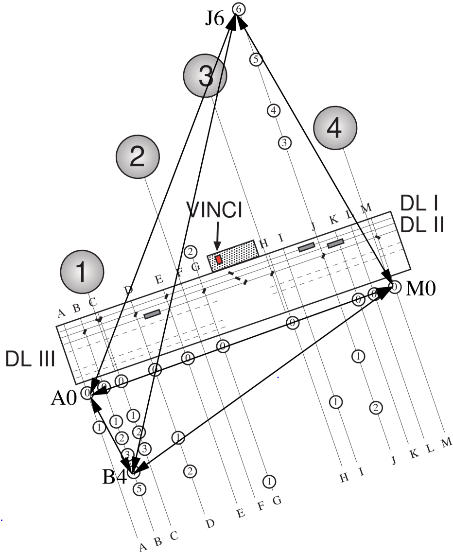
The rotation period of $\Theta^{1}$ Tau of 140 days would allow observations during two consecutive nights with a smearing effect of less than 5^∘. This makes it possible to reconfigure the array from one night to the other and to combine the data. However, since our model is also intended to describe a CM Cam type star at the location of $\Theta^{1}$ Tau, the CM Cam rotation period of only 16 days limits our combinable observing time to about 6 hours during only one night, with a smearing effect of less than about 5^∘. Due to the use of data taken during only one night, a reconfiguration of the array is not possible. In order to obtain a good coverage of the $uv$-plane despite of this, four telescopes are used for our simulation. The beams of any three of them can be fed to the AMBER instrument at any time. Four different triple configurations can then be used, of which three are independent. Not all baselines can be used at any time due to a limited range of the delay lines. Observations are simulated for 6 hours, 3 hours before meridian until 3 hours after meridian, with one measurement every 15 minutes on the next available triple configuration. Stations B4, J6, A0, and M0 were selected in order to achieve a maximum angular resolution at all position angles. Figure 3 shows a schematic view of the VLTI layout indicating the used array stations and baselines. Table 3 shows when each of the four possible triple configurations is used. Figure 4 shows the obtained coverage of the $uv$-plane. The selection of the telescope stations, as well as the calculation of the resulting coverage of the $uv$-plane considering the different restrictions was performed using observation preparation tools as described by Schöller (2000).

Figure 3: General layout of the VLTI. Shown are the positions of the 4 UTs, the 30 AT stations, the system of light ducts, the delay line tunnel with the currently existing three delay lines (three more are expected to be installed by mid 2003), and the interferometric lab with the currently used commissioning instrument VINCI. The arrows indicate the baselines which were used in our simulation, i.e. those between stations B4, J6, A0, and M0. The baseline length between stations B4 and J6 is 195.31 m, that between stations A0 and M0 is 144.0 m. North is at the top.

Table 3: The four different used triple configurations and the times when each of them is used, in hours relative to meridian.

B4 J6 A0	-3.00	-2.75	-2.50	-2.25	-1.75	-0.75
	0.25	1.25	2.25
B4 J6 M0	-1.25	-0.5	0.5	1.5	2.5
B4 A0 M0	-0.25	0.75	1.75	2.75
J6 A0 M0	-2.00	-1.50	-1.00	0.00	1.00	2.00
	3.00

Figure 4: Plot of the used coverage of the $uv$-plane for an object at a declination of $+16^{\circ}$ ($\Theta^{1}$ Tau). The size of each circle represents the size of a 1.8 m diameter VLTI Auxiliary Telescope. Four different telescopes are used at positions B4, J6, A0, M0. One out of four possible triple configurations is measured every 15 min. Tab. 3 shows which triple configuration was used at which time (based on observing restrictions of some baselines owing to limited delay line lengths).

Model results

Table 4: Reduced $\chi^{2}_{n}$ value, stellar diameter, and limb-darkening parameter $\alpha$ of that symmetric stellar disk without surface feature which fits best our simulated model star. The model star with parameters as given in Tab. 2 (diameter 2.6 mas) was used, as well as models for the same star at twice the distance (diameter 1.3 mas) and half the distance (diameter 5.2 mas).

Model star diameter (mas)	2.60	1.30	5.20
Stellar diameter (mas)	2.68	1.34	5.42
Limb-darkening parameter	0.52	0.56	0.62
Reduced $\chi^{2}$	16.0	0.1	186.7

Table 5: Accuracy ranges of our model parameters for a 5 $\sigma$ detection. The values are derived by varying each of the parameters and calculating the reduced $\chi^{2}_{n}$ value. The stellar diameter was adjusted to its best fitting value for every variation while all other parameters were kept constant.

Parameter	Model value	Accuracy range
Limb darkening par.	0.33	[0.27..0.41]
Spot diameter [mas]	0.5	]0..0.7]
Spot separation [mas]	0.70	[0.67..0.72]
Spot P.A. [degree]	90	[87..101]
Rel. offset intensity [%]	-1.0	[-0.8..-1.3]

Figure 5: Difference of our three model squared visibility amplitudes, triple amplitudes, and closure phase values (from top to bottom) to those of the best fitting symmetric stellar disk without a surface feature, in units of the size of the assumed error bar. The x-axis shows the time of the observation relative to meridian. Observations are simulated according to the triple configurations shown in Tab. 3.

The three squared visibility amplitudes, the triple amplitude, and the closure phase of our model star were calculated for each of the 25 observations which are listed in Tab. 3. The total number of independent data points of our simulation is 100. Errors were calculated according to the adopted precisions of the AMBER squared visibility amplitudes, triple amplitudes, and closure phases.

In order to determine whether the surface spot on our model star can be detected, the reduced $\chi^{2}_{n}$ value of the best fitting symmetric stellar disk without a surface spot to our spotted model star was calculated. The stellar diameter was treated as the only free parameter. Fits were performed for a range of assumed limb-darkening parameters. The minimum reduced $\chi^{2}_{n}$ value that was found during this procedure has been derived. In addition, these calculations were performed for the same model star shifted to twice its distance (diameter 1.3 mas) and half its distance (diameter 5.2 mas). Table 4 shows the resulting values. The asymmetric feature on our model star can be detected with a high significance ($\chi^{2}_{n}=16$). The same star with an apparent diameter of 1.3 mas can not be distinguished from a symmetric stellar disk ($\chi^{2}_{n}=0.1$), while the significance of the asymmetric feature on the 5.2 mas star is considerably higher ($\chi^{2}_{n}=187$). Figure 5 shows the differences of our simulated model star squared visibility amplitude, triple amplitude, and closure phase values to that of the best fitting symmetric stellar disk, in units of the assumed sizes of the error bars.

In order to estimate the accuracy of fitted model parameters, each of the parameters of our model star was varied until the reduced $\chi^{2}_{n}$ value reached a value of 5. The stellar diameter was adjusted to its best fitting value after every variation while all other parameters were kept constant. Table 5 shows the resulting accuracy ranges in comparison to our model as given in Tab. 2. Based on our assumptions, all model parameters can be derived with reasonable accuracy. The spot itself (0.5 mas diameter) is unresolved, with our conservative accuracy assumptions and a required 5 $\sigma$ detection. Thus, our model star can not be distinguished from a star with a smaller spot if the spot’s relative offset intensity remains in the range [-0.8%..-1.3%]. In other words, a smaller spot with a larger temperature difference relative to the unspotted photosphere can not be distinguished from a larger spot (up to 0.7 mas) with a smaller temperature difference. If, however, our model star is shifted to half its distance (stellar diameter 5.2 mas, spot diameter 1 mas), the spot diameter would be constrained to the range [0.85 mas..1.15 mas], and together with the constrains for the spot’s offset intensity, the spot temperature could be derived.

5 Summary and discussion

We have investigated the feasibility to image surface spots on magnetically active stars with the VLT interferometer. We used realistic model assumptions based on a Doppler image of the giant star CM Cam. Observations were considered which make use of the first generation VLTI instrument AMBER. All observing restrictions were taken into account, as for example the limited lengths of the delay lines. We used conservative assumptions for the accuracy and calibration uncertainty of the AMBER instrument. We have discussed that magnetically active single giants are the most promising candidate stars for interferometric imaging. We show by simulations of observations which are performed during only one night, that the surface feature on our model giant can be detected at a high significance level and estimate the accuracy of fitted spot parameters to be reasonably good. The combination of data taken during one night limits the rotational period of the star to about 15-20 days. For faster rotating stars, the rotation period could be modeled as an additional parameter. Our analysis shows as well that the angular diameter of our model star of 2.6 mas is at the lower limit for feasible interferometric studies of stellar surfaces using the VLTI with AMBER. We find, on the other hand, that the majority of stars for which the existence of surface features caused by magnetic activity is known or strongly suggested, have angular diameters smaller than 2 mas and, in addition, are located in the northern hemisphere. It would be desirable to initiate spectroscopic and photometric variability studies in the southern hemisphere, focusing on apparently large giants, as a preparation and source of complimentary information for VLTI measurements of stellar surface features. The VLTI, other ground based interferometers, and finally large space based UV interferometers promise to give us exciting new insights into magnetic and hydrodynamic activity of stars, with first results to be expected very soon.

Appendix A List of estimated angular diameters

Angular diameters were estimated for stars with known or expected surface structures in order to find suitable stars for interferometric observations of surface inhomogeneities. As a primary source, the ”Summary of Doppler images of late-type stars (www.aip.de/groups/activity/DI/summary) was used. In addition, a list of stars exhibiting photometric variations (Strassmeier et al. 1999) was used. For the latter stars, periods and radial velocities are known, but indirect surface images are not available. Some stars are listed in both of these sources. Furthermore, a list of slowly rotating single giants exhibiting Ca II variability (Choi et al. 1995) was used. These stars are expected to show surface structures but additional information on spot parameters is not available.

The following methods were employed in order to estimate stellar angular diameters:

1. The absolute diameter was calculated based on the effective temperature and bolometric luminosity. Tabulated values in Schmidt-Kaler (1982), based on the spectral type, were used for these quantities. The Hipparcos parallax was used to derive the angular diameter.

2. The empirical calibration for the angular diameter by Dyck et al. (1996) based on the spectral type and the K magnitude (Gezari et al. 1999) was used for giants. In case that the measured K magnitude includes a companion, the resulting error on the diameter is of the order of one.

3. The photometric period and the rotation velocity $v\sin i$ were used to derive the absolute radius of the star. This radius was converted into an angular diameter using the Hipparcos parallax. If the angle of inclination of the spot is not known, this estimate is a lower limit. In case that Doppler images exist, the angle of inclination given and the angular diameter was computed.

4. The CHARM (catalog of high angular resolution measurements, Richichi & Percheron 2002) was searched for measurements of angular diameters.

The errors on the estimated diameters can amount to up to a factor of about 2. Within these errors, the different estimates are usually consistent. Cases with larger deviations include the RS CVn variables CF Tuc, IN Vir, and II Peg, as well as the T Tauri stars V987 Tau, SU Aur, HT Lup, and V824 Tau.

Table 6: Estimated diameters for stars with known surface features. The sources are (Ref 2) ”Summary of Doppler images of late type stars”, www.aip.de/groups/activity/DI/summary (version from Dec. 18, 2001) and (Ref 1) the list in ”Starspot photometry with robotic telescopes”, Strassmeier et al. (1999). Listed are the star’s name, its HD number, the type of variability as given in the references, the parallax $\pi$ taken from Perryman & ESA (1997), the K magnitude from Gezari et al. (1999), if available, the spectral type, the rotation period P, the rotational velocity $v\sin i$, all as given in the references, the three different estimates of the angular diameters ($\theta_{1}$, $\theta_{2}$, $\theta_{3}$), and, finally, a measured value for the angular diameter, if available. The three different methods for the diameter estimates are explained in the text. The measured diameters are limb-darkened diameters, averaged over different measurements if more than one measured value was available. The references for the measured diameters are as follows. $\zeta$ And: Cohen et al. (1999), Hutter et al. (1989); V833 Tau: Chen & Simon (1997); SU Aur: Akeson et al. (2000, UD diameter in K-band); $\epsilon$ Aur: Nordgren et al. (2001); $\sigma$ Gem: Cohen et al. (1999) and Nordgren et al. (1999); 31 Com: Bell & Gustaffson (1989).

Name	HD	Type	$\pi$	SpT	K	P	P	$v\sin i$	$v\sin i$	$i$	$\theta_{1}$	$\theta_{2}$	$\theta_{3}$	$\theta_{m}$
						Ref 1	Ref 2	Ref 1	Ref 2
			mas		mag	d	d	km/s	km/s	deg	mas	mas	mas	mas
V640 Cas	123	SB	49.3	G8V				4.7			0.4
LN Peg		RS CVn	24.7	G8V	6.4	1.85		23			0.2		$\geq$ 0.2
$\zeta$ And	4502	RS CVN	18.0	K1III	1.4		17.64		41		2.1	2.6	$\geq$ 2.4	2.8
CF Tuc	5303	RS CVn	11.6	K4IV	5.3		2.8		35	64	0.9	0.5	0.2
AE Phe A	9528	W UMa	20.5	G0V			0.36		145	88	0.2		0.2
AE Phe B	9528	W UMa	20.5	F8V			0.36		95	88	0.2		0.1
XX Tri	12545	RS CVn	5.1	K0III		23.87	24	18.2	21	60	0.5		0.5
VY Ari	17433	RS CVn	22.7	K3IV		16.23		10			1.4		$\geq$ 0.7
UX Ari	21242	RS CVn	19.9	K0IV	3.8		6.44		39	60	0.9	0.8	1.1
V711 Tau	22468	RS CVn	34.5	K1IV	3.3	2.84	2.84	40	41	35	1.6	1.1	1.3
V471 Tau		BY Dra	21.4	K0V			0.52		91	90	0.2		0.2
EI Eri	26337	RS CVn	17.8	G5IV		1.91	1.95	50	51	46	0.6		0.4
YY Eri A	26609	W UMa	18.0	G9V			0.32		160	82	0.1		0.2
YY Eri B	26609	W UMa	18.0	G7V			0.31		110	82	0.2		0.1
V410 Tau	283518	WTTS	7.2	K4	7.5	1.87	1.87	77	77	70			0.2
EK Eri	27536	giant	15.8	G8III		306.9		1.5			1.5		$\geq$ 1.3
RY Tau	283571	CTTS	7.5	F8V	6.2			49			0.1
V987 Tau	283572	WTTS	7.8	G5III	6.8	1.53	1.55	78	78	48	0.6	0.2	0.2
DF Tau	283654	CTTS	25.7	M0	6.8		8.5		25	60			1.2
V833 Tau	283750	BY Dra	56.0	K5V		1.81		6.3			0.4		$\geq$ 0.1	$<10$
SU Aur	282624	CTTS	6.6	G2	5.8		3.09	66	64	80			0.3	1.9
YY Men	32918	FK Com	3.4	K2III			9.55		50	50	0.5		$\geq$ 0.4
$\epsilon$ Aur	31964		1.6	F0Ia	1.5						1.6	1.8		2.2
V1192 Ori	31993	giant	4.2	K2III		26.7		33			0.6		$\geq$ 0.7
V390 Aur	33798	giant	8.9	G8III		9.69		33			0.8		$\geq$ 0.5
AB Dor	36705	Single	66.9	K0V	4.7		0.51		91	60	0.5		0.7
V1355 Ori	291095	RS CVn	23.1	K1IV		3.87		46			1.1		$\geq$ 0.8
V1358 Ori	43989	RS CVn	20.1	G0III		3		42			1.6		$\geq$ 0.5
SV Cam	44982	RS CVn	11.7	G2V	7.4		0.59		117	90	0.1		0.2
CM Cam	51066	giant	3.6	G8III		16.0	16	47	47	60	0.3		0.6
$\sigma$ Gem	62044	RS CVn	26.7	K1III	1.7	19.62	19.4	27	27	60	3.2	2.3	3.0	2.4
TY Pyx	77137	RS CVn	17.9	G5V			3.20		35	88	0.2		0.4
IL Hya	81410	RS CVn	8.4	K1III		12.67	12.7	26.5	26.5	55	1.0		0.6
DX Leo	82443	BY Dra	56.4	K0V		5.43		5			0.4		$\geq$ 0.3
LQ Hya	82558	BY Dra	54.5	K2V		1.60	1.61	28	27	60	0.4		0.5
$\xi$ UMa B	98230	SB	137.0	K2V	2.3			2.8			1.0		$\geq$
DM UMa		RS CVn	7.2	K0III			7.5		26	40	0.8		0.4
HU Vir	106225	RS CVn	8.0	K0III		10.66	10.4	27	25	61	0.9		0.5
	111395	solar	58.2	G5V		15.8		2.9			0.5		$\geq$ 0.5
31 Com	111812	giant	10.6	G0III	3.3	6.96		57			0.9	1.0	$\geq$ 0.8	0.9
LW Hya		CBPN	7.5	G8III			0.76		90	45	0.7		0.1
IN Com	112313	RS CVn	0.8	G5III		5.90	5.91	67	67	45	0.1		0.1
37 Com	112989	giant	3.6	G8III				4			0.3
IN Vir	116544	RS CVn	8.8	K2III			8.23		24	60	1.2		0.4
FK Com	117555	FK Com	4.0	G2III		2.41	2.4	160	155	65	0.3		0.3
EK Dra	129333	single	29.5	G2V		2.60	2.6	17.5	17.3	60	0.3		0.3
UV CrB	136901	RS CVn	3.6	K2III		18.66		42			0.5		$\geq$ 0.5
UZ Lib		RS CVn	7.1	K0III	6.4	4.75	4.74	67	69	30	0.8	0.3	0.8
$\alpha$ CrB	139006	eclips	43.7	A0V	2.1			13			1.1
$\gamma$ CrB	140436	Maia	22.5	A0V		0.45		100			0.6		$\geq$ 0.2

Table 7: Table 6, continued

Name	HD	Type	$\pi$	SpT	K	P	P	$v\sin i$	$v\sin i$	$i$	$\theta_{1}$	$\theta_{2}$	$\theta_{3}$	$\theta_{m}$
						Ref 1	Ref 2	Ref 1	Ref 2
			mas		mag	d	d	km/s	km/s	deg	mas	mas	mas	mas
HT Lup		CTTS	6.3	K2III	6.5		3.9		40	70	0.9	0.3	0.2
$\delta$ CrB	141714	giant	19.7	G5III	2.7	57		5			1.5	1.3	$\geq$ 1.0
V2253 Oph	152178	RS CVn	2.1	K0III		22.07		28.8			0.2		$\geq$ 0.3
V824 Ara	155555	WTTS	31.8	G5IV			1.68		35	53	1.2		0.4
V889 Her	171488	solar	26.9	G0V		1.34		33			0.3		$\geq$ 0.2
PZ Tel	174429	WTTS	20.1	K0V			0.94		68	65	0.2		0.3
V1794 Cyg	199178	FK Com	10.7	G5III	3.2	3.34	3.32	67	71.5	50	0.8	1.1	0.6
ER Vul	200391	BY Dra	20.1	G0V			0.69		85	67	0.2		0.2
LO Peg		Single	39.9	K5V			0.42		69	35	0.3		0.4
V2075 Cyg	208472	RS CVn	6.4	G8III		22.42	22.4	19.7	21	45	0.6		0.8
HK Lac	209813	RS CVn	6.6	K0III		24.15	24.4	20	20	65	0.7		0.7
OU And	223460	giant	7.4	G0III		24.2		20			0.6		$\geq$ 0.7
IM Peg	216489	RS CVn	10.3	K2III	4.5	24.45	24.65	28.2	28	53	1.5	0.7	1.6
KU Peg	218153	RS CVn	5.3	G8III		25.9	25.3	23.1	28	50	0.5		0.8
II Peg	224085	RS CVn	23.6	K2V	4.6	6.73	6.72	23.1	23	61	0.2		0.8
V830 Tau	/	WTTS		M0	8.5		2.75		34	80		0.1
He 520		alpha Per	5.5	G5V			0.61		91	75			0.1
He 699		alpha Per	5.5	G2V			0.49		97	65			0.1
HII 3163		Pleiad	8.5	K0V			0.42		70	58			0.1
HII 686		Pleiad	8.5	K4V			0.40		64	51			0.1

Table 8: Estimated diameters for giants with predicted surface activity (Choi et al. 1995). A measured diameter is known only for $\Theta^{1}$ Tau, namely 2.6 mas (White & Feierman (1987).

Name	HD	$\pi$	SpT	K	P	$\theta_{1}$	$\theta_{2}$
		mas		mag	d	mas	mas
$\Theta^{1}$ Tau	28307	20.7	G9III	1.6	140	2.2	2.2
$\nu^{3}$ CMa	47442	7.0	K1III	1.9	183	0.8	1.9
19 Pup	68290	17.6	K0 III	2.6	159	1.9	1.4
	73598	4.5	G8III		159	0.4
39 CnC	73665	5.6	G9III	4.2		0.6	0.7
	73710	4.3	K0III	4.2	155	0.5	0.7
	73974	3.6	K0III		112	0.4
$\zeta$ Crt	102070	9.3	G8III	2.5	137	0.9	1.5
$\gamma$ Com	108381	19.2	K2III	1.9		2.7	2.2
	157527	10.8	G7III		147	1.0
$\iota$ Cap	203387	15.1	G8III	2.3	68	1.4	1.7