Photometric Mapping with ISOPHOT using the “P32” Astronomical Observation Template

Abstract

The “P32” Astronomical Observation Template (AOT) provided a means to map large areas of sky (up to 45$\times$45 arcmin) in the FIR at high redundancy and with sampling close to the Nyquist limit using the ISOPHOT C100 (3$\times$3) and C200 (2$\times$2) detector arrays on board ISO. However, the transient response behaviour of the Ga:Ge detectors, if uncorrected, can lead to severe systematic photometric errors and distortions of source morphology on maps. Here we describe the basic concepts of an algorithm which can successfully correct for transient response artifacts in P32 observations. Examples are given demonstrating the photometric and imaging performance of ISOPHOT P32 observations corrected using the algorithm.

1 INTRODUCTION

From the point of view of signal processing and photometry diffraction-limited mapping in the FIR with cryogenic space observatories equipped with photoconductor detectors poses a particular challenge. In this wavelength regime the number of pixels in detector arrays is limited in comparison with that in mid- and near-IR detectors. This means that more repointings needed to map structures spanning a given number of resolution elements. Due to the logistical constraints imposed by the limited operational lifetime of a cryogenic mission, this inevitably leads to the problem that the time scale for modulation of illumination on the detector pixels becomes smaller than the characteristic transient response timescale of the detectors to steps in illumination. The latter timescale can reach minutes.

Unless corrected for, the transient response behaviour of the detectors will lead to distortions in images, as well as to systematic errors in the photometry of discrete sources appearing on the maps. In general, these artifacts become more severe and more difficult to correct for at fainter levels of illumination, since the transient response timescales increase with decreasing illumination. Compared to the IRAS detectors, the ISOPHOT-C detectors (Lemke et al. 1996) on board the Infrared Space Observatory (ISO; Kessler et al. 1996) had relatively small pixels designed to provide near diffraction limiting imaging. ISOPHOT thus generally encountered larger contrasts in illumination between source and background than IRAS did, making the artifacts from the transient response more prominent, particularly for fields with faint backgrounds.

A further difficulty specific to mapping in the FIR with ISO was that, unlike IRAS, the satellite had no possibility to cover a target field in a controlled raster slew mode. This limited the field size that could be mapped using the spacecraft raster pointing mode alone, since the minimum time interval between the satellite fine pointings used in this mode was around 8 s. This often greatly exceeded the nominal exposure time needed to reach a required level of sensitivity (or even for many fields the confusion limit). Furthermore, the angular sampling and redundancy achievable using the fine pointing mode in the available time was often quite limited, so that compromises sometimes had to be made to adequately extend the map onto the background.

A specific operational mode for ISO - the “P32” Astronomical Observation Template (AOT) - was developed for the ISOPHOT instrument to alleviate these effects (Heinrichsen et al. 1997). This mode employed a combination of standard spacecraft repointings and rapid oversampled scans using the focal plane chopper. The technique could achieve a Nyquist sampling on map areas of sky ranging up to 45$\times$45 arcmin in extent (ca. 70$\times$70 FWHM resolution elements) on timescales of no more than a few hours. In addition to mapping large sources, the P32 AOT was extensively used to observe very faint compact sources where the improved sky sampling and redundancy alleviated the effects of confusion and glitching.

In all, over 6$\%$ of the observing time of ISO was devoted to P32 observations during the 1995-1998 mission, but the mode could not until now be fully exploited scientifically due to the lack of a means of correcting for the complex non-linear response behaviour of the Ge:Ga detectors. Here we describe the basic concept of a new algorithm which can successfully correct for the transient response artifacts in P32 observations. This algorithm forms the kernel of the “P32TOOLS” package, which is now publically available as part of the ISOPHOT Interactive Analysis package PIA (Gabriel et. al 1997; Gabriel & Acosta-Pulido 1999). Information on the algorithm, as well as the first scientific applications, can also be found in Tuffs et al. (2002). The user interface of P32TOOLS is described by Lu et al. (this volume). After a brief overview of relevant aspects of the P32 AOT in Sect. 2, we describe the semi-empirical model used to reproduce the transient response behaviour of the PHT-C detectors in Sect. 3. Sect. 4 describes the algorithms used to correct data. Examples demonstrating the photometric and imaging performance of ISOPHOT P32 observations are given in Sect. 5, based on maps corrected using P32TOOLS.

2 THE P32 AOT

The basic concept of the P32 AOT, in which imaging was achieved using a combination of standard spacecraft repointings and rapid oversampled scans using ISOPHOT’s focal plane chopper, is summarised in the contribution by C. Gabriel in this volume. There were two basic requirements, outlined in the original proposal for the AOT (Tuffs & Chini 1990) which led to the final design:

The first goal was to give ISOPHOT the capability of achieving a Nyquist sky sampling ($\Delta\Theta\,$=$\,\lambda$/2D = 17 arcsec at 100$\,\rm\mu m$) on extended sources subtending up to 50 resolution elements in a tractable observation time. As well as providing a unique representation of any arbitrary sky brightnesss distribution, this also improved the effective confusion limit in deep observations, which, in directions of low background was $\sim 100$ and 20 mJy rms at 200 and 100$\,\rm\mu m$, respectively, for ISOPHOT-C.

The second requirement was to achieve a redundancy in the observed data. This led to the sampling of each of a given set of sky directions by each detector pixel at different times. The redundancy was achieved in part by making several (at least 4) chopper sweeps at each spacecraft pointing direction. Further redundancy was achieved by having an overlap in sky coverage of at least half the chopper sweep amplitude between chopper sweeps made at successive spacecraft pointing directions in the Y spacecraft coordinate. Thus, a given sky direction was sampled on three different time scales by each detector pixel: on intervals of the detector non-destructive read interval, on intervals of the chopper sweep, and on intervals of the spacecraft raster pointings. Although the redundancy requirement was originally made to help follow the long term trends in detector responsivity during an observation, in practice it also proved very useful in removing effects caused by cosmic particle impacts (Gabriel & Acosta-Pulido 2000), the so-called “glitches”, from the data. This was especially important to optimise the sensitivity of deep observations using the C100 detector, which are generally limited by glitching rather than by confusion.

Both these requirements led to dwell times per chopper plateau which could be as low as 0.1 s. For a given sky brightness, this also had the consequence that the detector was generally read faster than in the other AOTs using the PHT-C detectors.

2.1 The P32 “natural grid”

The fact that the spacecraft pointing increment in Y was constrained to be a multiple of the chopper step interval means that a rectangular grid of directions on the sky can be defined such that all data taken during P32 measurement fine pointings will, to within the precision of the fine pointings, exactly fall onto the directions of the grid. This so-called P32 “natural grid” allows maps to be made without any gridding function, thus optimising angular resolution. The P32 natural grid is also a basic building block of the algorithm to correct for the transient response behaviour of the detector, as the algorithm solves for the intrinsic sky brightness in M$\times$N independent variables for a grid dimension of M$\times$N. An example of the almost perfect registration of data onto the grid is shown in Fig. 1.

Figure 1: Pointing directions observed towards Ceres at 105$\,{\mu}m$. The spacecraft raster dimension was $3\,\times\,3$ in the spacecraft coordinates $Y\,\times\,Z$. Sky sampling in $Y$ is achieved through a combination of chopper scans in $Y$ and repointings of the spacecraft. In $Z$ the sky sampling is determined alone by the spacecraft repointing interval. Each pointing direction for 11833 individual data samples for the central pixel of the C100 detector array is plotted as a cross. The rectangular grid is the “P32 natural grid” (see text) for this observation, on which the sky brightness distribution is to be solved. The grid sampling is $14.99\times 45.98$ arcsec. Only points with the on target flag set (i.e. not including slews) are plotted. The pointings typically lie within 1 arcsec of the centre of each pixel of the P32 natural grid.

All the example maps shown in this paper will be sampled without a gridding function on the P32 natural grid. This means that the data in each of the map pixels is independent. This is unlike the situation for most other maps calculated using PIA, where a gridding function is employed and so raw data can contribute to more than one map pixel.

3 TRANSIENT RESPONSE OF THE PHT-C DETECTORS

Gallium doped germanium photoconductor detectors exhibit a number of effects under low background conditions which create severe calibration uncertainties. The ISOPHOT C200 (Ge:Ga stressed) and especially the C100 (Ge:Ga) detectors have a complex non-linear response as a function of illumination history on timescales of $\sim 0.1-100$ sec, which depends on the absolute illumination as well as the changes in illumination. The following behaviour is seen in response to illumination steps:

• a rapid jump in signal, which however undershoots the asymptotic equilibrium response (often severely for the C100 array)

• a hook response (overshooting or undershooting on intermediate timescales of $\sim 1-10$ s)

• a slow convergence to the asymptotic equilibrium response of the detector on timescales of $\sim 10-100$ s

An example showing these effects for a staring observation is given in Fig. 2. Also seen are points discarded by the deglitching algorithm in PIA, marked by stars. Many glitches are accompanied by a longer lived “tail”. It is these tails that determine the ultimate sensitivity of the ISOPHOT C100 array.

Figure 2: Example of the transient response of a Ge:Ga detector following an upwards step to a constant level of illumination at 100$\,\rm\mu m$. The hook response is shown in the inset.

3.1 Semi-empirical detector model

Unlike the ISOCAM and ISOPHOT-S Si:Ge detectors, the transient response behaviour of the Ge:Ga detectors of ISOPHOT-C could not be described by the Fouks Schubert model (Schubert et al. 1995; Acosta-Pulido 1998). However, the effects observed in ISOPHOT-C can to some extent be qualitatively understood in terms of the build up of charge on the contacts between semiconductor and readout circuit, as modelled by Sclar (1984). Sclar’s model can be formulated as the superposition of three exponentials to describe the response of the detector to a step in illumination. The three timescales involved are a minimum requirement to reproduce the hook response and the long term approach to the asymptotic response. However, no theory exists to predict values for the constants in this representation, and thus they must be found empirically.

In practice it is a formidable and unsolved problem to extract the constants from in flight data for as many as three temporal components to the transient response behaviour. In this paper we describe an approximate solution involving a superposition of two exponentials, each with illumination-dependent constants. This was found to adequately represent the detector response on timescales greater than a few seconds, though it only approximately models the hook response. Our model can be viewed as a generalisation of the single exponential model developed for correction of longer stares by Acosta-Pulido, Gabriel & Castañeda (2000).

In the model considered here, the basic detector response $S$ to an instantaneous step in illumination from $S_{\rm\infty p}$ to $S_{\rm\infty}$ is given by the sum of a “slow” signal response $S_{1}$ and a “fast” signal response $S_{2}$ as:

$$S = S_{\rm 1}+S_{\rm 2}$$ (1)

$$S_{\rm 1} = (1-\beta_{\rm 1})\,S_{\rm\infty}\,(1-{\rm exp}[-t/\tau_{\rm 1}])\,+\,S_{\rm 01}\,{\rm exp}[-t/\tau_{\rm 1}]$$ (2)

$$S_{\rm 2} = \beta_{\rm 2}\,S_{\rm\infty}\,(1-{\rm exp}[-t/\tau_{\rm 2}])\,+\,S_{\rm 02}\,{\rm exp}[-t/\tau_{\rm 2}]$$ (3)

$S_{\rm 01}$ and $S_{\rm 02}$ are signals corresponding to the slow and fast response components immediately following the illumination step. $S_{\rm 01}$ and $S_{\rm 02}$ are related to the corresponding signals immediately prior to the illumination step, $S_{\rm 1p}$ and $S_{\rm 2p}$, which contain the information about the illumination history. $S_{\rm 01}$ and $S_{\rm 02}$ are specified by the jump conditions:

$$S_{\rm 01} = \beta_{\rm 1}\,(S_{\rm\infty}-S_{\rm\infty p})+S_{\rm 1p}$$ (4)

$$S_{\rm 02} = S_{\rm 2p}$$ (5)

The model is thus specified by four primary parameters: the slow and fast timescales $\tau_{\rm 1}$ and $\tau_{\rm 2}$, the “jump” factor $\beta_{\rm 1}$ and a constant of proportionality for the fast response $\beta_{\rm 2}$. In order to obtain satisfactory model fits to complex illumination histories, each of these primary parameters had to be specified as monotonic functions of illumination, each with three subsiduary parameters:

$$\beta_{\rm 1}=\beta_{\rm 10}\,+\,\beta_{\rm 11}\,*\,S_{\rm\infty}^{\beta_{\rm 12}}$$ (6)

$$\tau_{\rm 1}=\tau_{\rm 10}\,+\,\tau_{\rm 11}\,*\,S_{\rm\infty}^{\tau_{\rm 12}}$$ (7)

$$\beta_{\rm 2}=\beta_{\rm 20}\,+\,\beta_{\rm 21}\,*\,S_{\rm\infty}^{\beta_{\rm 22}}$$ (8)

$$\tau_{\rm 2}=\tau_{\rm 20}\,+\,\tau_{\rm 21}\,*\,S_{\rm\infty}^{\tau_{\rm 22}}$$ (9)

Thus 12 subsiduary parameters in all are needed to characterise the transient response behaviour of the detectors. In addition, the initial starting state of the detector, given by the values of $S_{\rm 1p}$ and $S_{\rm 2p}$ immediately prior to the start of the mapping observation, must be specified.

3.2 Determination of model parameters

The parameterisation of the illumination dependence of the primary parameters $\tau_{\rm 1}$, $\beta_{\rm 1}$, $\tau_{\rm 2}$ and $\beta_{\rm 2}$ was made in engineering units (V/s), rather than in astrophysical units such as MJy/sr. Thus, it was assumed that there is no dependence of the detector response on the wavelength of the IR photons reaching the detector. Since the individual pixels of the C100 and the C200 arrays behave as independent detectors, each of the 12 parameters of the detector model had to be separately determined for each detector pixel.

The “slow” primary parameters $\tau_{\rm 1}$ and $\beta_{\rm 1}$ were found from fits to the detector response to fine calibration source (FCS) exposures. An example is given in Fig. 3. The model fit to the signal response on time scales ranging from a few seconds up to the duration of the FCS exposure depends mainly on the values of $\tau_{\rm 1}$ and $\beta_{\rm 1}$.

Figure 3: Example of a model fit (curve) to the response of the central pixel of the C100 array to a constant FCS illumination starting at $t=0$ s. Prior to the FCS illumination the detector was viewing blank sky. The horizontal line indicates the fitted value of the illumination. No data was recorded in the first two seconds following FCS switch-on.

A database of values for $\tau_{\rm 1}$ and $\beta_{\rm 1}$ was built up for a wide variety of FCS illuminations, allowing the dependence of $\tau_{\rm 1}$ and $\beta_{\rm 1}$ on illumination to be determined according to Eqns. 6$\,\&\,$7. An example showing the illumination dependence of $\beta_{\rm 1}$ for the central pixel of the C100 array is given in Fig. 4. The solid line is the fitted illumination dependence of $\beta_{\rm 1}$ used to find the values of the parameters $\beta_{\rm 10}$, $\beta_{\rm 11}$ and $\beta_{\rm 12}$ used in the model. A corresponding plot for the illumination dependence of $\tau_{\rm 1}$ is given in Fig. 5.

Figure 4: Values of the parameter $\beta_{\rm 1}$ for the central pixel of the C100 array found from fits to the detector response to FCS exposures, plotted versus FCS illumination. The solid line is a fit of the function $\beta_{\rm 1}=\beta_{\rm 10}+\beta_{\rm 11}S_{\rm\infty}^{\beta_{\rm 12}}$ with $\beta_{\rm 10}=2.12$, $\beta_{\rm 11}=-1.82$, and $\beta_{\rm 12}=0.022$. These are the parameters adopted for th model giving the default illumination dependence of $\beta_{\rm 1}$ for this pixel.

Figure 5: As Fig. 4, but for the parameter $\tau_{\rm 1}$. The solid line is a fit of the function $\tau_{\rm 1}=\tau_{\rm 10}+\tau_{\rm 11}S_{\rm\infty}^{\tau_{\rm 12}}$ with $\tau_{\rm 10}=6.92s$, $\tau_{\rm 11}=4.28$, and $\tau_{\rm 12}=-1.22$. These are the parameters adopted for the model giving the default illumination dependence of $\tau_{\rm 1}$ for this pixel.

Figure 6: Values of the parameter $\beta_{\rm 2}$ for the central pixel of the C100 array found from self calibration optimisation of the model on observations of standard point source calibrators, plotted versus illumination. The solid line is a fit of the function $\beta_{\rm 2}=\beta_{\rm 20}+\beta_{\rm 21}S_{\rm illum}^{\beta_{\rm 22}}$ with $\beta_{\rm 20}=-0.543$, $\beta_{\rm 21}=0.723$, and $\beta_{\rm 22}=-0.0103$, where $S_{\rm illum}$ is the known illumination of the detector pixel due to the point source calibrator. These are the parameters adopted for the model giving the default illumination dependence of $\beta_{\rm 2}$ for this pixel.

Figure 7: As Fig. 4, but for the parameter $\tau_{\rm 2}$. The solid line is a fit of the function $\tau_{\rm 2}=\tau_{\rm 20}+\tau_{\rm 21}S_{\rm illum}^{\tau_{\rm 22}}$ with $\tau_{\rm 20}=14.89\,s$, $\tau_{\rm 21}=-14.24$, and $\tau_{\rm 22}=0.01025$. These are the parameters adopted for the model giving the default illumination dependence of $\tau_{\rm 2}$ for this pixel.

At shorter timescales the response is primarily determined by the “fast” primary parameters $\tau_{\rm 2}$ and $\beta_{\rm 2}$. However, the FCS exposures could not be used to find $\tau_{\rm 2}$ and $\beta_{\rm 2}$ since no data was recorded in the first two seconds following the detector switch-on. This is also the reason why the hook response is not seen in Fig. 3. Furthermore, there is very probably a non-negligible timescale needed by the FCS to reach its final operating temperature. Therefore, the “fast” parameters (with timescales $\sim\,$0.1$\,\leq\,\tau\,\leq\,\sim\,$5 s) were found using a self calibration technique (described in Sect. 4.2), operating on co-added repeated chopper sweeps crossing standard point source calibrators. Observations of standard point source calibrators of a range of flux densities allowed the dependence of $\tau_{\rm 1}$ and $\beta_{\rm 1}$ on illumination to be determined according to the parameterisation of Eqns. 8$\,\&\,$9. Examples showing the illumination dependence of $\beta_{\rm 2}$ and $\tau_{\rm 2}$ for the central pixel of the C100 array are given in Figs. 6 and 7, respectively.

4 THE P32TOOLS ALGORITHM

In a standard reduction of ISOPHOT data using the interactive analysis procedures of PIA, the analysis is made in several irreversible steps, starting with input “edited raw data” at the full time resolution, and finishing with the final calibrated map. To correct for responsivity drift effects, however, it is necessary to iterate between a sky map and the input data at full time resolution. This different concept required a completely new data reduction package. In its development phase, and for the determination of the detector model parameters, this data reduction package was run as a set of IDL scripts. It was later interfaced to PIA as P32TOOLS using a GUI interface as described elsewhere in this volume.

There are three basic elements to the P32TOOLS concept. The first step is signal conditioning, which aims to provide a stream of signal values, each with an attached time, from which artifacts such as glitches, dark current, and non-linearity effects have been removed, but which retains the full imprint of the transient response of the detector to the illumination history at the sharpest available time resolution. We will refer to such a stream of signals as the “signal timeline”.

The second step is the transient correction itself, which is an iterative process to determine the most likely sky brightness distribution giving rise to the observed signals. This is a non-linear optimisation problem with the values of sky brightness as variables. For large maps several hundred independent variables are involved.

Lastly, there is the calculation of calibrated transient corrected maps. This entails the conversion from V/s to MJy/sr, flat fielding, and the coaddition of data from different detectors pixels. Within P32TOOLS, this third stage is performed using standard PIA software, and is therefore not described further here.

4.1 Signal Conditioning

The processing steps for signal conditioning are as follows:

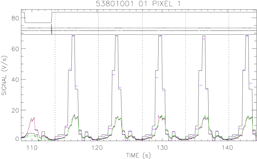
Figure 8: Detail from a signal timeline from an observation of the standard calibrator Ceres, observed in the C105 filter. The green line shows the fit to the observed signal (shown in red) from pixel 1 of the C100 array, as found by the P32TOOLS algorithm for correction of the transient response behaviour of this pixel. 5 chopper sweeps, each comprising 13 pointing directions (“chopper plateaus”) are shown, divided by vertical dotted lines separated in time by a duration of 6.1s for each sweep. The upper line in the figure shows the fine pointing flag; whereas the first chopper sweep shown was made while the spacecraft was slewing between fine pointings (flag value 0), the subsequent chopper sweeps were made on a single fine pointing (flag value 1). The remaining horizontal lines denote masks at the full time resolution of the data denoting glitches, readout status and whether or not a solution for the illumination could be found by the algorithm. The overall solution for the sky illumination for this detector pixel is given by the histogram in black. As described in the text, this overall solution is calculated from a combination of individual solutions for illumination on each successive chopper plateau, which are shown here as purple bars. For the very brightest sources, as shown in this example, the derived illuminations can be up to a factor of 6 brighter than the raw data for pixels in the C100 array. In this example the hook response is well seen in each chopper sweep at the 9th and 10th chopper plateaus.

1. Edited Raw Data is imported, after having been corrected in PIA for the integration ramp non-linearity.

2. The specification of chopper phase in the data is checked and corrected where necessary.

3. The pointing is established from the instantaneous satellite pointing information, unlike PIA which uses the commanded pointing. This also establishes the pointing directions on the slews between the spacecraft fine pointings. Internally defined “on target flags” are set for each spacecraft fine pointing direction, and the central direction and sampling intervals directions for the P32 “natural grid” (see Sect. 2) are established.

4. The integration ramps are differentiated and the data is corrected for dark current and dependence of photometry on reset interval, using standard calibration parameters taken from PIA.

5. Systematic variations of the signal according to position in the integration ramps are removed from the data. This process is called “signal relativisation” within P32TOOLS. In contrast to the default pipeline or PIA analysis, this allows the use of all non-destructive reads, as well as providing a more complete signal timeline for use in the correction of the transient behaviour of the detector. The “signal relativisation” is applied such that signal variations due to the transient response behaviour are preserved.

6. Random noise is determined by examining the statistics of the signals on each chopper plateau. This is necessary due to the high readout rates of the detectors in many P32 observations. Otherwise, the determination of noise from individual readout ramps, as done in a standard PIA analysis, would be insufficiently precise.

7. Spikes are detected and removed from the data in a first-stage deglitching procedure. This operates at the full time resolution of the data given by the non-destructive read interval.

8. A second stage deglitching procedure is performed, operating at the time resolution of the chopper plateau (which comprise of at least 16 non-destructive read intervals). This procedure (described by Peschke & Tuffs in this volume) removes any long lived glitch “tails” following the spikes detected in the first-stage deglitch.

4.2 Transient Correction

The calculation to correct for the transient response behaviour is made separately for each detector pixel. The kernel of the procedure is to solve for the illumination corresponding to the signal on each chopper plateau. This is done in a binary chop scheme for set values of the 12 detector parameters. The values for $S_{\rm 1p}$ and $S_{\rm 2p}$ needed to solve for illumination on each chopper plateau are calculated from the response of the model to the preceding illumination history.

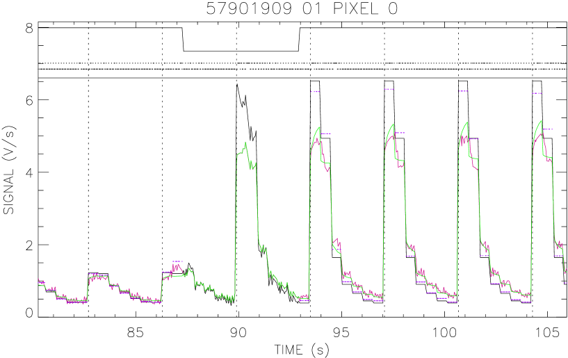
Figure 9: Detail from a timeline of signal versus time from another observation of Ceres, this time observed in the C160 filter using the C200 detector array. The key to the plot is as given in the caption to Fig. 8. This example shows the transition from a spacecraft fine pointing for which the chopper is sweeping through beam sidelobes to a fine pointing where the chopper samples the beam kernel. In this case the red line corresponding to the data is not seen during the intervening spacecraft slew, as it is exactly overplotted by the green line showing the fit to the data (see text). The chopper sweeps on the second fine pointing encompassing the beam kernel show a typical enhancement of the source-background contrast induced by the algorithm for correction of the transient response.

After solving for the illumination on the current chopper plateau, the found value is combined with previous solutions encountered for the same sky position from previous chopper plateaus viewing the same sky direction. The response of the detector pixel to the illumination history is recalculated and a solution is found for the illumination viewed on the next chopper plateau. This procedure is continued until all the signal timeline has been processed. Then a second pass through the data can be made, and so on, until the overall solution for the sky brightness distribution no longer changes. The goodness of the solution is quantified through a value for $\chi^{\rm 2}$, calculated from a comparison between the model fit and the signal timeline. The random uncertainties assigned to each signal sample in the timeline can optionally be recalculated from the self consistency of solutions for the illumination found in a given sky direction. Examples of model fits to the signal timeline are shown in Fig. 8 for the C100 detector and in Fig. 9 for the C200 detector.

The algorithm can also be used for datasets for which the readout rate was too rapid to allow all the data to be transmitted to the ground. In such cases the illumination history can still be determined at all times on fine pointings, even where there are gaps in the signal timeline. On slews, the illumination history during the gaps are either interpolated in time, or taken from the nearest previously solved direction on the P32 natural grid.

For most observations using the C200 detector, and observations of moderate intensity sources made using the C100 detector, good fits to the entire unbroken signal timeline can be obtained for each detector pixel. For observations of bright sources using the C100 detector, however, it is often necessary to break up the solutions into smaller segments, according to the distribution of the sources in the field mapped. This is best achieved by solving separately for the portions of the signal timeline passing through the bright sources. The most conservative processing strategy, appropriate for observations using the C100 detector of complex brightness distributions with high source to background contrast, is to break up the calculation into time intervals corresponding to individual spacecraft fine pointings. This means that no processing of the slews is required.

Several processing options are available, to optimise solutions for the particular characteristics of each dataset:

Determination of detector starting state

The default operation of the program is to assume that the detector is in equilibrium at the start of the observation, viewing the sky direction corresponding to the first detector plateau. This corresponds to the case $S_{\rm 1p}\,=\,S_{\rm 01}\,=\,S_{\rm\infty}$ and $S_{\rm 1p}\,=\,0$. This will very rarely be the case, however, since an FCS measurement which may not be perfectly matched to the sky brightness will have been made just seconds prior to the start of the spacecraft raster.

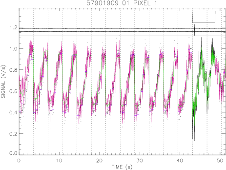
Figure 10: A further detail from the timeline of signal versus time for the observation of Ceres in the C160 filter. This time the fit to the data for the very first fine pointing is shown, to illustrate the fit to the switch-on transient behaviour of the detector (see Sect. 4.2) For a constant repeated illumination pattern in each chopper sweep, both the data (red) and the fit (green) gradually move lower through the first half minute of the observation.

Therefore, the program can optionally find a solution for the detector starting state, as characterised by the values of $S_{\rm 1p}$ and $S_{\rm 2p}$ immediately prior to the start of the first chopper plateau. This is done by solving for $S_{\rm 1p}$ and $S_{\rm 2p}$ for a fixed $S_{\rm\infty}$ on the first plateau, where $S_{\rm\infty}$ is determined from the last chopper plateau in the first spacecraft pointing to view the same sky direction. The timeline for the first spacecraft pointing is then repeatedly processed until a stable solution for $S_{\rm 1p}$ and $S_{\rm 2p}$ prior to the first plateau is found. This option was found particularly useful for data taken with the C200 detector. An example of a model fit to a timeline where a solution for the detector starting states was found in this way is shown in Fig. 10.

“Self calibration” of detector parameters

In order to determine the primary detector parameters $\beta_{\rm 2}$ and $\tau_{\rm 2}$ in the first instance, “a self calibration” processing technique was used by which any of the 12 detector parameters (Sect. 3.1) could be determined from observations of bright sources. Sources of any arbitrary brightness distribution and position can be used. However, to determine the detector parameters for the “fast” response of the detector, point source calibrators of known brightness were used, and the solutions for $\tau_{\rm 2}$ and $\beta_{\rm 2}$ were additionally constrained by the requirement that the solutions for illumination were consistent with the known flux densities of the calibrators.

The self calibration procedure works by simply repeating the optimisation process for different subsets of the 12 detector parameters, specified by the user. Each combination of detector parameters produces an individual solution for the sky brightness distribution, as well as a value for $\chi^{\rm 2}$. A search is made in the parameter space of the detector parameters until a minimum is found in $\chi^{\rm 2}$. This is a lengthy process, however, making it advisable to perform self calibrations on limited portions of the timeline. This is often chosen to correspond to a single spacecraft pointing where the chopper sweeps for the detector pixel being investigated pass through bright structure. The process can be further accelerated in cases that the repeated chopper sweeps through a source give the same repeated signal pattern. Then, the optimisation can be performed on an average of the coadded chopper sweeps performed on a single spacecraft pointing. This latter technique is referred to in P32TOOLS as a “composite self calibration”. Some examples of the useage of the self calibration procedure are given in this volume by Schulz et al. (2002).

Processing of slews

The calculation of the illumination history for data taken during the slews is less straightforward than for data taken during the spacecraft fine pointings. This is because the instantaneous pointing directions during slews are effectively at random positions with respect to the P32 natural grid. Therefore, the use of solutions for the sky brightness distribution on the P32 natural grid found from analysis of previous fine pointings will in general lead to inaccuracies in the determination of the illumination history during the slews. There are two main approaches which can be adopted to counter this problem.

The first is to solve for the illumination not over a chopper plateau, but for individual readouts in the signal timeline during the slew. This automatically provides a solution in which the model fit exactly matches the data, as there is only one fitted data point for each determined illumination. An example is given in the fit to the signal timeline for the C200 detector shown in Fig 9. This approach is useful for observations of bright structured sources in which the variations in illumination with position on the slew on timescales of a chopper plateau exceed the signal to noise on individual data samples. It is the default processing option for the C200 detector.

In cases of low signal to noise, and for all instances where not all data are transmitted to the ground, solving for the average illumination on each chopper plateau is a preferable technique. Otherwise, the values of $S_{\rm 1p}$ and $S_{\rm 2p}$ calculated just prior to the first chopper plateau on the next fine pointing can be wildly inaccurate, which can corrupt the solutions for the remainder of the signal timeline of the observation. Processing on a plateau by plateau basis is the default processing option to calculate the illumination history during slews for observations with the C100 detector.

5 PHOTOMETRIC PERFORMANCE

In general the corrections in integrated flux densities made by the algorithm depend on the source brightness, structure, the source/background ratio, and the dwell time on each chopper plateau. The largest corrections are for bright point sources on faint backgrounds.

Here we give as an example results achieved for the faint standard star HR 1654. This source was not used in the determination of the detector model parameters, so it constitutes a test of the photometric performance of ISOPHOT in its P32 observing mode. The derived integrated flux densities, with and without correction for the transient response behaviour of the C100 detector, were compared in Fig. 11 with predicted flux densities from a stellar model. The corrected photometry is in reasonable agreement with the theoretical predictions. As expected, there is a trend for observations with larger detector illuminations to have larger corrections in integrated photometry.

Figure 11: The measured integrated flux densities of the faint standard star HR 1654 plotted against the predicted flux densities from a stellar model. The observations were done in various filters using the C100 detector. The photometry derived with and without processing with P32TOOLS is shown with stars and crosses, respectively.

A good linear correlation is also seen between integrated flux densities of Virgo cluster galaxies (Tuffs et al. 2002), derived from P32 ISOPHOT observations processed using the P32TOOLS algorithm, and flux densities from the IRAS survey (Fig. 12). The interpretation of these measurements constitutes the first science application (Popescu et al. 2002) of P32TOOLS algorithm. The ISOPHOT observations of Virgo cluster galaxies were furthermore used to derive the ratios of fluxes measured by ISO to those measured by IRAS. The ISO/IRAS ratios were found to be 0.95 and 0.82 at 60 and 100$\,\rm\mu m$, respectively, after scaling the ISOPHOT measurements onto the COBE-DIRBE flux scale (Tuffs et al. 2002).

Figure 12: Integrated and colour-corrected flux densities of Virgo cluster galaxies measured in the ISO C100 filter versus the corresponding flux densities measured by IRAS in its 100$\,\rm\mu m$ band (taken from Fig. 7 of Tuffs et al. 2002). The dotted line represents the relation ISO/IRAS=0.82.

Figure 13: Brightness profiles along the Y spacecraft direction through the standard star HR 1654 at 100$\,\rm\mu m$. The solid line represents the brightness profile obtained after processing with P32TOOLS, while the dotted line shows the profile derived from identically processed data, but without correction for the transient response of the detector.

Fig. 13 shows an example of a brightness profile through HR 1654 at 100$\,\rm\mu m$, for data processed with and without the responsivity correction. Some 95$\%$ of the flux density has been recovered by P32TOOLS. Without the correction, some 30$\%$ of the integrated emission is missing and the signal only reaches 50$\%$ of the peak illumination. The local minimum near 60 arcsec in the Y offset is a typical hook response artifact, where the algorithm has overshot the true solution. This happens for rapid chopper sweeps passing through the beam kernel. This is a fundamental limitation of the detector model, which, as described in Sect. 3.1, does not correctly reproduce the hook response on timescales of up to a few seconds. This problem is particularly apparent for downwards illumination steps. The only effective antidote is to mask the solution immediately following a transition through a bright source peak. Another effect of the inability to model the hook response is that the beam profile becomes somewhat distorted. This also has the consequence, that for observations of bright sources, the measured FWHM can become narrower than for the true point spread function, as predicted from the telescope optics and pixel footprint. An example of an extremely bright point source showing this effect is given in Figs. 14 & 15, depicting maps of Ceres in the C105 filter, respectively made without and with the correction for the transient response of the C100 detector.

Figure 14: Contour map of Ceres in the C105 filter after responsivity drift correction. 50 linear contours have been plotted between 33 and 2519 MJy/sr. Measured integrated flux density after background subtraction is $98.4$ Jy $\pm\,0.2$ Jy (random) $\,\pm\,6\%$ (systematic). The actual flux density of this standard calibrator (from a stellar model) is 109 Jy.

Figure 15: Contour map of Ceres in the C105 filter without correction for the transient response behaviour of the detector. 50 linear contours have been plotted between 11.5 and 334 MJy/sr. Measured integrated flux density after background subtraction is $28.0$ Jy $\pm\,0.07$ Jy (random) $\,\pm\,4\%$ (systematic).

Despite the limitations due to the lack of a proper modelling of the hook response, the algorithm can effectively correct for artifacts associated with the transient response on timescales from a few seconds to a few minutes. This is illustrated in Figs. 16 & 17 by the maps of the interacting galaxy pair KPG 347 in the C200 filter (again, after and before correction for the transient response of the detector, respectively). The uncorrected map shows a spurious elongation in the direction of the spacecraft Y coordinate, which is almost completely absent in the corrected map. If uncorrected, such artifacts could lead to false conclusions about the brightness of FIR emission in the outer regions of resolved sources. Also visible in the corrected map is a trace of a beam sidelobe.

Figure 16: The interacting galaxy pair kpg 347 observed in the C200 filter after processing with P32TOOLS.

Figure 17: The interacting galaxy pair kpg 347 with identical processing, except that the correction for the transient response behaviour of the detector has been omitted

The image of M 101 in Fig. 18, made using the C100 detector with the C100 filter, is given as a state of the art example of what can be achieved with a careful interactive processing of P32 data using P32TOOLS. In addition to the transient response corrections and a masking of residual hook response artifacts, a time dependent flat field has been applied. The spiral structure of the galaxy, with embedded HII region complexes and a component of diffuse interarm emission can clearly be seen.