Simultaneous single-pulse observations of radio pulsars

In this paper, we present a study of orthogonal polarization modes in the radio emission of PSR B1133+16, conducted within the frame of simultaneous, multi-frequency, single-pulse observations. Simultaneously observing at two frequencies (1.41 GHz and 4.85 GHz) provides the means to study the bandwidth of polarization features such as the polarization position angle. We find two main results. First, that there is a high degree of correlation between the polarization modes at the two frequencies. Secondly, the modes occur more equally and the fractional linear polarization decreases towards higher frequencies. We discuss this frequency evolution and propose propagation effects in the pulsar magnetosphere as its origin.

1 Introduction

Simultaneous multi-frequency observations of radio pulsars in full polarization are proving to be a very powerful tool for investigating the puzzling pulsar emission problem. In Karastergiou et al. (khk01 (2001), hereafter Paper I), we provided a detailed introduction into the history of multi-frequency observations and the ongoing efforts to construct an emission theory which will be both self-consistent and consistent with the abundance of observational information from pulsars. We also laid out the guidelines for simultaneous polarimetric observations between different telescopes by presenting our time-aligning and re-binning techniques.

Observations of the Vela pulsar by Radhakrishnan & Cooke (rc69 (1969)) showed the radiation to be highly linearly polarized and to be emitted from near the magnetic pole. The observed position angle (PA) reflects the instantaneous projection of the dipolar magnetic field lines on the plane of the sky and thus changes with the rotation of the star (the so-called rotating vector model, RVM). Later, Manchester et al. (mth75 (1975)) demonstrated that the percentage polarization could vary between 0 and 100% across pulse longitude, that significant circular polarization was often present and, perhaps most surprisingly, that significantly different PAs were seen at the same pulse longitude. These PA jumps were often very close to $90^{o}$ and thus the linear polarization occurred in ‘orthogonally polarized modes’ (OPM). The existence of OPM was a key discovery (Backer & Rankin 1980). By using simple arguments it can be shown that the presence of OPM acting together in the emission process can reduce the fraction of polarization observed (Stinebring et al. 1984, McKinnon 1997, McKinnon & Stinebring 1998). Subsequently, single pulse polarization studies by Gil & Lyne (1995) demonstrated that OPM was responsible for the low percentage polarization and very complicated PA variations in the integrated profile of PSR B0329+54, in which two simple OPM modes existed.

Melrose & Stoneham (ms77 (1977)) and Barnard & Arons (ba86 (1986)) proposed a model for the OPM in pulsars by considering propagation effects (refraction) which cause rays in the two natural modes of the plasma to split. This has been further developed by McKinnon (mck97 (1997)) who showed that a model involving birefringence of the two modes can explain the observed pulse width and fractional polarization changes with frequency.

In this paper, we shall focus on the polarization behaviour of PSR B1133+16 and use the results to draw some general conclusions about the pulsar emission processes.

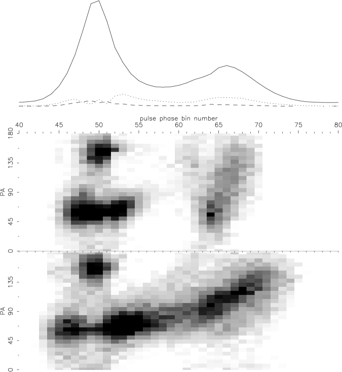
Figure 1: The total power profile of PSR B1133+16 is shown together with the linear polarization at two frequencies; the dotted line corresponds to 1.41 GHz and the dashed line to 4.85 GHz [TOP]. The grey-scale PA histograms follow, at 4.85 GHz [MIDDLE] and 1.41 GHz [BOTTOM]. The darker areas in the grey-scale histograms correspond to more frequent values of PA, as they occur on a single-pulse basis. The PA values are not absolute.

Figure 2: PA-PA plot for phase bin 50. The distribution of the PA values for each frequency is also plotted.

2 Observations

On 2000 January 4, we used the Effelsberg 100-m telescope at 4.85 GHz and the Lovell 76-m telescope in Jodrell Bank at 1.41 GHz to observe PSR B1133+16 (see von Hoensbroech et al. hkk98 (1998), von Hoensbroech & Xilouris hx97 (1997) for details on the Effelsberg observing system and Paper I and Gould & Lyne gl98 (1998) for the Jodrell Bank system). Both telescopes were simultaneously on source for $\approx 93$ minutes or 4778 pulse periods. For the purpose of this paper, we also make use of Jodrell Bank data observed at 610 MHz (Gould & Lyne gl98 (1998)), as well as Effelsberg 2.69 GHz data (Paper I) from different epochs. The data from each telescope were calibrated and converted into the EPN-format (Lorimer et al. ljs98 (1998)), after being aligned and re-binned to a common reference frame and temporal resolution (in this case 1.16 ms per bin), as described in Paper I.

3 Results

3.1 The behaviour of modes with frequency

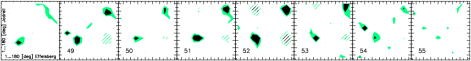
Figure 3: A sequence of phase bins from the leading component of the pulse. Each frame consists of a PA-PA histogram for the phase bin in the lower left corner, as identified in Fig. 1, and shows the deviation of the observed PA pairs from the null hypothesis, weighted by the calculated $\sigma$ (see explanation in text).

Fig. 1 shows the integrated pulse profile at 1.41 GHz along with the linear polarization at both frequencies. In this paper we ignore the circular polarization, which is generally low throughout the pulse. Fig. 1 also shows the PA distribution as a function of phase in a grey-scale representation at both 1.41 GHz and 4.85 GHz. It can be seen that at the peak of the first component two orthogonal modes are clearly present at both frequencies. In the second component one mode dominates at 1.4 GHz but two modes can be seen at the higher frequency. Integrated profiles like these have been used to question the broad-band nature of OPM (e.g Stinebring et al. 1984); for the first time, however, we can use the simultaneous nature of our data to determine this issue.

At each of the two observed frequencies we compute the PA only if the flux density of the linear polarization exceeds twice the noise. We do this for each phase bin of every pulse; an example of one such bin near the peak of the first component is given in Fig 2. Under incoherent addition of the OPMs, the PA is only permitted to take one of two discrete values, exactly $90^{o}$ apart. In this bin, it is clear that the orthogonal PA modes are present at both frequencies, although the spread in PA of each mode is somewhat larger than one would expect from a delta-function convolved with instrumental noise (Stinebring et al. 1984, McKinnon & Stinebring 1998,). Two clear results are apparent in the figure. First, at 1.41 GHz the ratio of pulses in the two modes is 65:35 whereas at 4.85 GHz this ratio is 54:46. The modes are occurring more equally at 4.85 GHz and the fractional linear polarization has also decreased. Secondly, all four possible combinations between the two modes at the two frequencies occur, i.e. four islands are visible in Fig. 2. Given the difference in the bimodal distributions at the two frequencies, such a distribution of points in the plot must arise, even in the case when there is no correlation between the PAs of the two frequencies. Hence, it is not readily clear from Fig. 2 whether the cases of agreement and disagreement of OPM, represented by the four islands, suggest a high or low degree of correlation between the frequencies. Obviously, the correlation is not perfect since the individual distributions are different — which is an important result already – but some degree of correlation may still exist. We have to test whether the distribution of points in the PA-PA plot can be attributed to some random combination of PA-values at different frequencies, or whether the knowledge of the polarization mode at one frequency allows one to predict the mode at the other to some extent. We test the degree of correlation by comparing the observed PA-PA distributions to the null hypothesis that the two frequencies are completely uncorrelated.

We re-bin our PA distributions into histograms of 12 bins across the $180^{o}$ range of PA values. By doing this we create a 2-dimensional $12\times 12$ histogram $Obs(i,j)$, which represents the number of occurrences of all possible PA-PA pairs as they are observed. Then we use Monte Carlo simulations (MCS) to randomly combine our two observed PA distributions. We repeat this process a large number of times, thus obtaining another 2-dimensional histogram $Null(i,j)$, similar to $Obs(i,j)$, where the population in each square bin is the mean result from all MCS iterations. At the same time, we can calculate the standard deviation, $\sigma$, representing the statistical fluctuations which we can expect in each square bin of the null hypothesis case. We now subtract the null hypothesis $Null(i,j)$ from the observed 2-d histogram $Obs(i,j)$, and compare this difference with the expected noise in each square bin, $\sigma$. This will give us the significance in units of $\sigma$ that an observed number of points $Obs(i,j)$ is not consistent with the null-hypothesis of no correlation.

Such a null hypothesis test can only be applied reasonably to bins where we observe bimodal PA distributions at both frequencies, as other cases cannot be distinguished from a random combination of PA values per se. Hence, in Fig. 3 we plot a 2-d PA-PA histogram only for the phase bins of the leading pulse component where the individual PA distributions are bimodal. The solid areas denote a difference between $Obs(i,j)$ and $Null(i,j)$ of more than $3\sigma$ surrounded by a lighter coloured area marking differences exceeding $2\sigma$. Hatched areas denote differences of less than $-3\sigma$ surrounded again by lighter coloured area of $-2\sigma$ significance. We can clearly see that when one mode occurs at one frequency, it also prefers to occur at the other frequency: the same modes combine much more times than the null hypothesis of no-correlation predicts (black areas on the x=y diagonal).

In cases where the modes disagree, one mode does not necessarily favour a value at the other frequency that is different by exactly $90^{o}$. On the contrary, for most of the time the PA value at the other frequency seems to be completely unrelated, resulting in a distribution of points outside the diagonal islands that is mostly consistent with the null hypothesis. This is an interesting result with possible implications on the widths of PA distributions at given frequencies. Only in few cases is a lack of points observed when compared to the null hypothesis (hatched areas), supporting an increased degree of correlation between the frequencies. We note that Fig. 3 does not change qualitatively by using grids coarser than $12\times 12$.

The results in this section therefore show that there is a high degree of correlation between the two frequencies. The same mode tends to dominate at both frequencies and to this extent OPM is broadband in nature. At the same time, the modes occur more equally and the fractional polarization is lower at the higher frequency. This will be discussed in more detail below.

3.2 The $x$ and $s$ parameters

According to Stinebring et al. (scr84 (1984)), the emission we receive at any pulse phase is the instantaneous, incoherent superposition of the two OPMs. The PA value is that of the strongest mode. Two important parameters can be constructed to investigate the strength and behaviour of the modes.

The first parameter, $x$, represents the relative popularity of the PA of one mode with respect to the other. By studying the individual PA distributions for each frequency, it is possible to identify the OPMs across the phase bins of the pulse. We can identify the PA of each mode in each bin $i$ by finding the mean PA (or tracing the PA swing when the mode seems absent) and identifying a PA range of $\approx 30^{o}$ each side of the mean, which corresponds to the typical width of the PA histograms, as shown in Fig. 2. $M_{1}$ is the number of pulses where the PA corresponds to mode 1 and $M_{2}$ the same for mode 2. For each of the frequencies we studied the occurrence of $M_{1}$ and $M_{2}$ at every pulse phase bin.

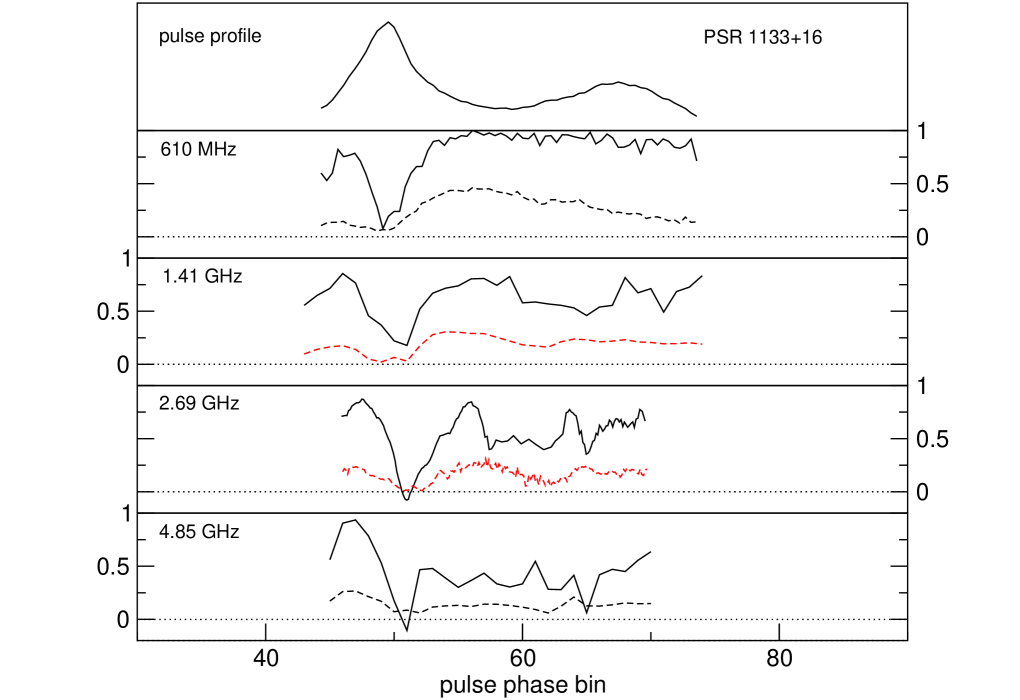
Figure 4: The parameter $x$ [solid line] and $|s|$ [dashed line] across the phase bins of PSR B1133+16 for four different frequencies. There is a general trend for both $x$ and $s$ to become closer to zero toward higher frequencies.

From the values of $M_{1}$ and $M_{2}$ we have calculated for each phase bin, we construct $x=\frac{M_{1}-M_{2}}{M_{1}+M_{2}}$. The value of $x$ depends on the relative values of $M_{1}$ and $M_{2}$. If they are equal, $x$ will obviously be zero. On the other hand, if one of them is larger than the other, $x$ will diverge from zero, 1 and $-1$ being the extreme cases, where only one of the modes is present.

The second parameter is $s$, which represents the relative strengths of the modes and varies from $-1$ to 1 in a similar fashion to $x$. $s$ is defined as $s=\frac{S_{1}-S_{2}}{S_{1}+S_{2}}$, where each phase bin is assumed to be the incoherent sum of two 100% orthogonally polarized modes with individual flux densities $S_{1}$ and $S_{2}$ (Stinebring et al. scr84 (1984)). In the case where the modes have a negligible fraction of circular polarization (as is the case here), then $|s|=L/I$, where $L$ is the linear polarization and $I$ the total power.

We used the simultaneously observed data to study the behaviour of $x$ and $s$ with frequency. We noticed that, although they are both phase dependent, they generally seem to have values closer to zero at 4.85 GHz than at 1.41 GHz (Fig. 4). We then used other observations of PSR B1133+16 to see if this behaviour is consistent at other frequencies. The Jodrell Bank 610 MHz data and the Effelsberg 2.69 GHz data, which are of comparable length to the simultaneous data, clearly show this remarkable trend. In other words, the times $M_{2}$ or $M_{1}$ determine the PA become more equal towards higher frequencies, while at the same time mode 2 is becoming closer in strength to mode 1 ($s$ closer to 0).

4 Discussion

In the case of PSR B1133+16 we have found the following trends of the OPMs:

• OPMs have a spectral dependence: the polarized intensities of the modes ($s$) and their frequency of occurrence ($x$) are becoming comparable at higher frequencies;

• we observe phase bins that simultaneously show a high value of $x$ and a low value of $s$;

• despite the spectral evolution, we find a strong connection between the two frequencies: the same polarization modes prefer to appear together;

• different modes, however, do appear at the two frequencies, implying a degree of de-correlation.

The first two trends are also supported by the 610 MHz and 2.69 GHz data.

How well do these observational trends fit in with the model of superposed orthogonal modes? A high value of $x$ implies that a given mode dominates most of the time. A low value of $s$ implies that the difference in the average strengths of these two modes are rather small. These two facts can only be reconciled by postulating that the amplitudes of the two modes are highly correlated (McKinnon & Stinebring 1998). A physical mechanism which can induce mode splitting with a high degree of amplitude correlation is birefringence and this means of mode creation in the relativistic pulsar plasma was proposed by Barnard & Arons (1986).

We also observe that, at least in this pulsar, $x$ decreases more rapidly with frequency than does $s$. This clearly implies that the correlation coefficient is decreasing with increasing frequency even though the relative strengths of the modes change rather little. One observational consequence of this is that we would expect that the distribution of linear polarization in the single pulses has a rather low dispersion when the correlation coefficient is high, compared to when the correlation coefficient is low. This is indeed seen in the data; the distribution of linear polarization is broader in the single pulses observed at 4.85 GHz.

We therefore surmise that the relative strength of the modes is set by the polarization of the input beam to the bi-refringent medium and that this is largely constant with frequency. The frequency trend in the observed value of $s$ arises from the refractive index of the modes being frequency dependent - at some ‘critical’ frequency and above, the beams overlap, causing a decrease in $s$. In this pulsar, $s$ changes rather little with frequency, as do the mode–separated pulse widths between 1.41 GHz and 4.85 GHz and presumably the critical frequency lies near 1.4 GHz. In most other pulsars, however, the critical frequency seems to lie above 5 GHz (Xilouris et al.xk96 (1996)).

The third and fourth conclusions we reach, together with the fact that total power is well correlated in our data (as was the case for PSR B0329+54 in Paper I), also point towards propagation effects. They support the idea that OPMs, which could be created by the splitting of the two natural orthogonal polarization modes in the magnetosphere by a propagation effect like birefringence, endure further propagation effects that change their relative strengths. One explanation could be that the absorption (e.g. cyclotron absorption) of one or other of the modes is frequency dependent with the higher frequencies more affected than lower frequencies. A change in relative strength could switch the dominant mode. The obvious manifestations of this are the clearly seen OPM disagreements at the two frequencies.

A further observational test of propagation effects and the superposed mode ideas comes from the circular polarization. One expects that a given mode is associated with a given sign of circular polarization and that there is therefore a strong correlation between the dominant mode and the sign of circular polarization in the single pulse data. Given that we see a high correlation between mode occurrences at different frequencies, will we also see a correlation between the handedness of the circular polarization? Simultaneous, multi-frequency, single–pulse observations are ideal as a test to identify propagation effects at work on the radiation traveling through the plasma in the pulsar magnetosphere.

- (1) Backer D. C. & Rankin J. M., 1980, ApJS, 42, 143
- (2) Barnard J. J. & Arons J., 1986, ApJ, 302, 138
- (3) Gil J. A., Lyne A. G., 1995, MNRAS 276, L55
- (4) Gould D. M. & Lyne A. G., 1998, MNRAS, 301, 235
- (5) Karastergiou A., von Hoensbroech A., Kramer M., et al., 2001, A&A, 379, 270
- (6) Gupta Y., Gangadhara R. T., Rathnashree N., 2000, PASP Conference Series, 202, 249
- (7) Lorimer D. R., Jessner A., Seiradakis J. H., et al., 1998, A&AS 128, 541
- (8) Manchester R. N., Taylor J. H., & Huguenin G. R., 1975, ApJ, 196, 83
- (9) McKinnon M. M., 1997, ApJ, 475, 763
- (10) McKinnon M. M. & Stinebring D. R., 1998, ApJ, 502, 883
- (11) Melrose D. B. & Stoneham R. J., 1977, Proceedings of the Astronomical Society of Australia, 3, 120
- (12) Radhakrishnan V. & Cooke D. J., 1969, Astrophys. Lett., 3, 225
- (13) Stinebring D. R., Cordes J. M., Rankin J. M., et al., 1984, ApJS 55,247
- (14) von Hoensbroech A., Kijak, J., & Krawczyk, A. 1998, A&A, 334, 571
- (15) von Hoensbroech A. & Xilouris K. M., 1997, A&AS, 126, 121
- (16) Xilouris K. M., Kramer M., Jessner A., et al., 1996, A&A, 309, 481