A model independent approach to the dark energy equation of state

Abstract

The consensus of opinion in cosmology is that the Universe is currently undergoing a period of accelerated expansion. With current and proposed high precision experiments it offers the hope of being able to discriminate between the two competing models that are being suggested to explain the observations, namely a cosmological constant or a time dependent ‘Quintessence’ model. The latter suffers from a plethora of scalar field potentials all leading to similar late time behaviour of the universe, hence to a lack of predictability. In this paper, we develop a model independent approach which simply involves parameterizing the dark energy equation of state in terms of known observables. This allows us to analyse the impact dark energy has had on cosmology without the need to refer to particular scalar field models and opens up the possibility that future experiments will be able to constrain the dark energy equation of state in a model independent manner.

I Introduction

Current cosmological observations suggest that the energy density of the universe is dominated by an unknown type of matter, called ’dark energy’, PERL ; RIES ; BOOM1 ; BOOM2 ; DASI ; 2df . If correct, it is characterized by a negative value for the equation of state parameter $w$ (close to $-1$) and is responsible for the present accelerating expansion of the Universe. The simplest dark energy candidate is the cosmological constant, but in alternative scenarios the accelerated phase is driven by a dynamical scalar field called ‘Quintessence’ WETT ; RATRA ; CALD ; FERRE . Although recent analysis of the data provides no evidence for the need of a quintessential type contribution CORAS ; BEAN ; HANN , the nature of the dark energy remains illusive. In fact the present value of its equation of state $w_{Q}$ is constrained to be close to the cosmological constant one, but the possibility of a time dependence of $w_{Q}$ or a coupling with cold dark matter for example LUCA cannot be excluded. Recent studies have analysed our ability to estimate $w_{Q}$ with high redshift object observations WAGA ; NEWMAN1 ; NEWMAN2 ; ALCANIZ ; CALVAO and to reconstruct both the time evolution of $w_{Q}$ HUT00 ; ASTIER ; BARG ; GOL ; MAO ; WELLA ; WELLB as well as the scalar field potential $V(Q)$ HUT99 ; SAINI ; CHI . An alternative method for distinguishing different forms of dark energy has been introduced in SAHNI , but generally it appears that it will be difficult to really detect such time variations of $w_{Q}$ even with the proposed SNAP satellite KUJ ; MAOR . One of the problems that has been pointed out is that, previously unphysical fitting functions for the luminosity distance have been used, making it difficult to accurately reproduce the properties of a given quintessence model from a simulated data sample HUT00 ; WELLB ; GERKE . A more efficient approach consists of using a time expansion of $w_{Q}$ at low redshifts. For instance in ASTIER ; WELLA ; WELLB a polynomial fit in redshift space $z$ was proposed, while in EFS ; GERKE a logarithmic expansion in $z$ was proposed to take into account a class of quintessence models with slow variation in the equation of state. However even these two expansions are limited, in that they can not describe models with a rapid variation in the equation of state, and the polynomial expansion introduces a number of unphysical parameters whose value is not directly related to the properties of a dark energy component. The consequence is that their application is limited to low redshift measurements and cannot be extended for example to the analysis of CMB data. An interesting alternative to the fitting expansion approach, has recently been proposed Huterer , in which the time behavior of the equation of state can be reconstructed from cosmological distance measurements without assuming the form of its parametrization. In spite of the efficiency of such an approach, it does not take into account the effects of the possible clustering properties of dark energy which become manifest at higher redshifts. Hence its application has to be limited to the effects dark energy can produce on the expansion rate of the universe at low redshifts. On the other hand, it has been argued that dark energy does not leave a detectable imprint at higher redshifts, since it has only recently become the dominant component of the universe. Such a statement, however, is model dependent, on the face of it there is no reason why the dark energy should be negligible deep in the matter dominated era. For instance CMB observations constrain the dark energy density at decoupling to be less then 30 per cent of the critical one BEAN2 . Such a non negligible contribution can be realized in a large class of models and therefore cannot be a priori excluded. Consequently it is of crucial importance to find an appropriate parametrization for the dark energy equation of state that allows us to take into account the full impact dark energy has on different types of cosmological observations. In this paper we attempt to address this very issue by providing a formula to describe $w_{Q}$, that can accommodate most of the proposed dark energy models in terms of physically motivated parameters. We will then be in a position to benefit from the fact that the cosmological constraints on these parameters will allow us to infer general information about the properties of dark energy.

II Dark energy equation of state

The dynamics of the quintessence field $Q$ for a given potential $V$ is described by the system of equations:

$$\ddot{Q}+3H\dot{Q}+\frac{dV}{dQ}=0,$$ (1)

and

$$H^{2}=\frac{8\pi G}{3}\left[\rho_{m}+\rho_{r}+\frac{\dot{Q}^{2}}{2}+V(Q)\right],$$ (2)

where $\rho_{m}$ and $\rho_{r}$ are the matter and radiation energy densities respectively and the dot is the time derivative. The specific evolution of $w_{Q}(a)$, where $a$ is the scale factor, depends on the shape of the potential, however there are some common features in its behaviour that can be described in a model independent manner and which allow us to introduce some physical parameters. As a first approach, we notice that a large number of quintessence models are characterized by the existence of the so called ’tracker regime’. It consists of a period during which the scalar field, while it is approaching a late time attractor, evolves with an almost constant equation of state whose value can track that of the background component. The necessary conditions for the existence of tracker solutions arising from scalar field potentials has been studied in CALD ; STEIN . In this paper, we consider a broad class of tracking potentials. These include models for which $w_{Q}(a)$ evolves smoothly, as with the inverse power law ZLATEV , $V(Q)\sim 1/Q^{\alpha}$ (INV) and the supergravity inspired potential BRAX , $V(Q)\sim 1/Q^{\alpha}e^{Q^{2}/2}$ (SUGRA). Late time rapidly varying equation of states arise in potentials with two exponential functions BARRE , $V\sim e^{-\alpha Q}+e^{\beta Q}$ (2EXP), in the so called ‘Albrecht & Skordis’ model ALB (AS) and in the model proposed by Copeland et al. COPE (CNR). To show this in more detail, in fig.1 we plot the equation of state obtained by solving numerically Eq. (1) and Eq. (2) for each of these potentials.

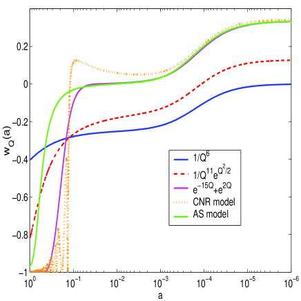
Figure 1: Evolution of $w_{Q}$ against the scale factor for an inverse power law model (solid blue line), SUGRA model (BRAX ) (dash red line), two exponential potential model (BARRE ) (solid magenta line), AS model (ALB ) (solid green line) and CNR model (COPE ) (dot orange line).

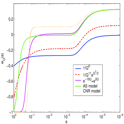
Figure 2: Plot of $w_{Q}^{p}(a)$ best fit for different potentials

There are some generic features that appear to be present, and which we can make use of in our attempts to parameterize $w_{Q}$. For a large range of initial conditions of the quintessence field, the tracking phase starts before matter-radiation equality. In such a scenario $w_{Q}(a)$ has three distinct phases, separated by two ‘phase transitions’. Deep into both the radiation and matter dominated eras the equation of state, $w_{Q}(a)$, takes on the values $w_{Q}^{r}$ and $w_{Q}^{m}$ respectively, values that are related to the equation of state of the background component $w_{B}$ through CALD ; STEIN :

$$\ w_{Q}\approx\frac{w_{B}-2(\Gamma-1)}{2\Gamma-1},$$ (3)

where $\Gamma=V^{\prime\prime}V/(V^{\prime})^{2}$ and $V^{\prime}\equiv dV/dQ$ etc. For the case of an exponential potential, $\Gamma=1$, with $w_{Q}=w_{B}$, but in general $w_{Q}\neq w_{B}$. Therefore if we do not specify the quintessence potential the values of $w_{Q}^{r}$ and $w_{Q}^{m}$ should be considered as free parameters.

The two transition phases can each be described by two parameters; the value of the scale factor $a_{c}^{r,m}$ when the equation of state $w_{Q}$ begins to change and the width $\Delta_{r,m}$ of the transition. Since $\Gamma$ is constant or slowly varying during the tracker regime, the transition from $w_{Q}^{r}$ to $w_{Q}^{m}$ is always smooth and is similar for all the models (see fig. 1). To be more precise, we have found that $a_{c}^{r}\sim 10^{-5}$ and $\Delta_{r}\sim 10^{-4}$ during this transition, the former number expected from the time of matter-radiation equality and the latter from the transition period from radiation to matter domination. However, when considering the transition in $w_{Q}$ from $w_{Q}^{m}$ to the present day value $w_{Q}^{0}$, we see from fig. 1 that this can be slow ($0<a_{c}^{m}/\Delta_{m}<1$) or rapid ($a_{c}^{m}/\Delta_{m}>1$) according to the slope of the quintessence potential. For instance in models with a steep slope followed by a flat region or by a minimum, as in the case of the two exponentials, the AS potential or the CNR model, the scalar field evolves towards a solution that approaches the late time attractor, finally deviating from the tracking regime with the parameter $\Gamma$ rapidly varying. In contrast the inverse power law potential always has a slower transition since $\Gamma$ is constant for all times. Given these general features we conclude that the behavior of $w_{Q}(a)$ can be explained in terms of functions, $w_{Q}^{p}(a)$, involving the following parameters: $w_{Q}^{0}$, $w_{Q}^{m}$, $w_{Q}^{r}$, $a_{c}^{m}$ and $\Delta_{m}$. The authors of BASS have recently used an expansion in terms of a Fermi-Dirac function in order to constrain a class of dark energy models with rapid late time transitions. In what follows we find that a generalisation of this involving a linear combination of such functions allows for a wider range of models to be investigated. To be more precise, we propose the following formula for $w_{Q}^{p}(a)$:

$$w_{Q}^{p}(a)=F_{1}f_{r}(a)+F_{2}f_{m}(a)+F_{3},$$ (4)

with

$$f_{r,m}(a)=\frac{1}{1+e^{-\frac{a-a_{c}^{r,m}}{\Delta_{r,m}}}}.$$ (5)

The coefficients $F_{1}$, $F_{2}$ and $F_{3}$ are determined by demanding that $w_{Q}^{p}(a)$ takes on the respective values $w_{Q}^{r}$, $w_{Q}^{m}$, $w_{Q}^{0}$ during radiation ($a_{r}$) and matter ($a_{m}$) domination as well as today ($a_{0}$). Solving the algebraic equations that follow we have:

$$F_{1}=\frac{\left(w_{Q}^{m}-w_{Q}^{r}\right)\left(f_{m}(a_{0})-f_{m}(a_{r})\right)-\left(w_{Q}^{0}-w_{Q}^{r}\right)\left(f_{m}(a_{m})-f_{m}(a_{r})\right)}{\left(f_{r}(a_{m})-f_{r}(a_{r})\right)\left(f_{m}(a_{0})-f_{m}(a_{r})\right)-\left(f_{r}(a_{0})-f_{r}(a_{r})\right)\left(f_{m}(a_{m})-f_{m}(a_{r})\right)},$$ (6)

$$F_{2}=\frac{w_{Q}^{0}-w_{Q}^{r}}{f_{m}(a_{0})-f_{m}(a_{r})}-F_{1}\frac{f_{r}(a_{0})-f_{r}(a_{r})}{f_{m}(a_{0})-f_{m}(a_{r})},$$ (7)

$$F_{3}=w_{Q}^{r}-F_{1}f_{r}(a_{r})-F_{2}f_{m}(a_{r}),$$ (8)

where $a_{0}=1$, and the value of and $a_{r}$ and $a_{m}$ can be arbitrarily chosen in the radiation and matter era because of the almost constant nature of $w_{Q}$ during those eras. For example in our simulations we assumed $a_{r}=10^{-5}$ and $a_{m}=10^{-3}$. In table 1 we present the best fit parameters obtained minimizing a chi-square for the different models of fig.1, and in fig.2 we plot the associated functions $w_{Q}^{p}(a)$. It is encouraging to see how accurately the Fermi-Dirac functions mimic the exact time behavior of $w_{Q}(a)$ for the majority of the potentials. In fig.3 we plot the absolute value of the difference $\Delta w(a)$ between $w_{Q}(a)$ and $w_{Q}^{p}(a)$. The discrepancy is less then $1\%$ for redshifts $z<10$ where the energy density of the dark energy can produce observable effects in these class of models and it remains below $9\%$ between decoupling and matter-radiation equality. Only the CNR case is not accurately described by $w_{Q}^{p}(a)$ due to the high frequency oscillations of the scalar field which occur at low redshift as it fluctuates around the minimum of its potential. In fact these oscillations are not detectable, rather it is the time-average of $w_{Q}(a)$ which is seen in the cosmological observables, and can be described by the corresponding $w_{Q}^{p}(a)$. There are a number of impressive features that can be associated with the use of $w_{Q}^{p}(a)$ in Eq. (4). For instance it can reproduce not only the behavior of models characterized by the tracker regime but also more general ones. As an example of this in fig.4 we plot $w_{Q}^{p}(a)$ corresponding to three cases: a K-essence model MUKA (blue solid line); a rapid late time transition PARKER (red dash-dot line) and finally one with an equation of state $w_{Q}^{0}<-1$ (green dash line). The the observational constraints on $w_{Q}^{0}$, $w_{Q}^{m}$, $w_{Q}^{r}$, $a_{c}^{m}$ and $\Delta_{m}$ lead to constraints on a large number of dark energy models, but at the same time it provides us with model independent information on the evolution of the dark energy. It could be argued that the five dimensional parameter space we have introduced is too large to be reliably constrained. Fortunately this can be further reduced without losing any of the essential details arising out of tracker solutions in these Quintessence models. In fact nucleosynthesis places tight constraints on the allowed energy density of any dark energy component, generally forcing them to be negligible in the radiation era MEL ; YA . The real impact of dark energy occurs after matter-radiation equality, so we can set $w_{Q}^{r}=w_{Q}^{m}$. Consequently we end up with four parameters: $w_{Q}^{0}$, $w_{Q}^{m}$, $a_{c}^{m}$ and $\Delta_{m}$. Although they increase the already large parameter space of cosmology, they are necessary if we are to answer fundamental questions about the nature of the dark energy. The parameters make sense, if $w_{Q}(a)$ evolves in time, we need to know when it changed ($a_{c}^{m}$), how rapidly ($\Delta_{m}$) and what its value was when it changed ($w_{Q}^{m}$). Neglecting the effects during the radiation dominated era it proves useful to provide a shorter version of Eq. (4), in fact since we can neglect the transition from radiation to matter dominated eras, then the linear combination Eq. (4) can be rewritten as :

$$w_{Q}^{p}(a)=w_{Q}^{0}+(w_{Q}^{m}-w_{Q}^{0})\times\frac{1+e^{\frac{a_{c}^{m}}{\Delta_{m}}}}{1+e^{-\frac{a-a_{c}^{m}}{\Delta_{m}}}}\times\frac{1-e^{-\frac{a-1}{\Delta_{m}}}}{1-e^{\frac{1}{\Delta_{m}}}}.$$ (9)

As we can see in fig.5, the relative difference between the exact solution $w_{Q}(a)$ of the Klein-Gordon equation and Eq. (9) is smaller than $5\%$ for redshifts $z<1000$, therefore it provides a very good approximation for the evolution of the quintessence equation of state. Both Eq. (4) and Eq. (9) are very useful in that they allow us to take into account the clustering properties of dark energy (see for instance DAVE ) and to combine low redshift measurements with large scale structure and CMB data. We would like to point out that one of the key results in this paper is the fact that our expansion for the equation of state allows for a broader range of redshift experiments than has previously been proposed.

Table 1: Best fit values of the parameters of the expansion  (4).

	$w_{Q}^{0}$	$w_{Q}^{m}$	$w_{Q}^{r}$	$a_{c}^{m}$	$\Delta_{m}$
INV	-0.40	-0.27	-0.02	0.18	0.5
SUGRA	-0.82	-0.18	0.10	0.1	0.7
2EXP	-1	0.01	0.31	0.19	0.043
AS	-0.96	-0.01	0.31	0.53	0.13
CNR	-1.0	0.1	0.32	0.15	0.016

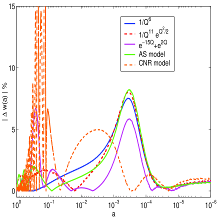
Figure 3: Absolute value of the difference between $w_{Q}(a)$ and $w_{Q}^{p}(a)$ for the models of fig.1.

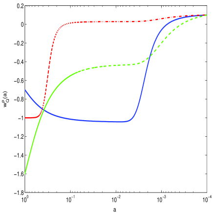
Figure 4: Time evolution of $w_{Q}^{p}(a)$ as in the case of K-essence (blue solid line), late time transition (red dash-dot line) end with $w_{Q}^{o}<-1$ (green dash line).

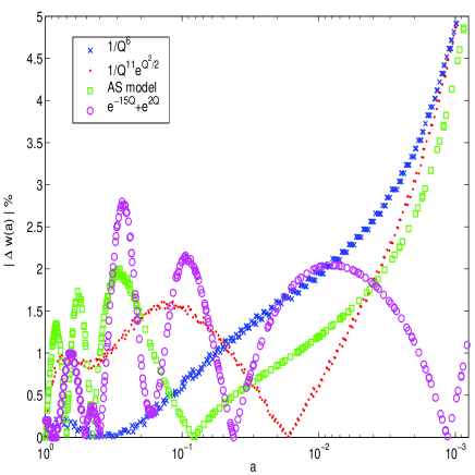
Figure 5: Absolute value of the difference between $w_{Q}(a)$ and the low redshift formula Eq. (9) for the models of fig.1.

III Conclusions

The evidence for a present day accelerating universe appears to be mounting, and accompanied with it is the need to understand the nature of the dark energy that many believe to be responsible for this phenomenon. Of the two possibilities proposed to date, a cosmological constant or a Quintessence scalar field, the latter suffers in that there are a plethora of models that have been proposed, all of which satisfy the late time features, that of an accelerating universe. Yet there is no definitive particle physics inspired model for the dark energy therefore an other route should be explored, trying to determine the equation of state that the dark energy satisfies in a model independent manner. If this were to work it would allow us to discuss the impact dark energy has had on cosmology without the need to refer to particular dark energy scenario. In this paper, we have begun addressing this approach. We have introduced a parameterization of the dark energy equation of state $w_{Q}^{p}(a)$ which involves five parameters and shown how well they reproduce a wide range of dark energy models. By estimating their value from cosmological data we can constrain the dark energy in a model independent way. This could be important in future years when high precision CMB and large scale structure observations begin to probe medium to large redshifts, regions where differences in the features of the Quintessence models begin to emerge. Although the low redshift data indicate that it is currently impossible to discriminate a cosmological constant from a Quintessence model, moving to higher redshifts may result in evidence for a time varying equation of state in which case, we need to be in a position to determine such an equation of state in a model independent manner. We believe this paper helps in this goal.

- (1) Perlmutter, S. et al. 1999, Astrophys. J. , 517, 565
- (2) Riess, A. et al. 1999, Astrophys. J. , 117, 707
- (3) De Bernardis, P. et al. 2000, Nature 404, 955-959
- (4) Netterfield, C. B. et al. 2001, astro-ph/0104460
- (5) Pryke, C. et al. 2001, Astrophys. J. , 568, 46
- (6) Efstathiou, G. et al. 2001, astro-ph/0109152
- (7) Wetterich, C. 1988, Nucl. Phys. B 302, 645
- (8) Ratra, B. and Pebbles, P.J.E. 1988, Phys. Rev. D 37, 3406
- (9) Caldwell, R. R., Dave, R., and Steinhardt, P. J. 1998, Phys. Rev. Lett. 80, 1582-1585
- (10) Ferreira, P. G, and Joyce, M. 1998, Phys. Rev. D58, 023503
- (11) Corasaniti, P. S. and Copeland, E. J. 2002, Phys. Rev. D65, 043004
- (12) Bean, R. and Melchiorri, A. 2002, Phys. Rev. D65, 041302
- (13) Hannestad, S. and Mortsell, S. 2002, astro-ph/020509
- (14) Amendola, L. et al. 2002, astro-ph/0205097
- (15) Waga, I. and Miceli, A. P. 1999, Phys. Rev. D59, 103507
- (16) Newman, J. A. and Davis, M. 2000, Astrophys. J. Lett., 534, L11
- (17) Newman, J. A. and Davis, M. 2002, Astrophys. J. , 564, 567
- (18) Lima, J. A. S. and Alcaniz, J. S. 2002, Astrophys. J. , 566, 15
- (19) Calvao, M. O., de Mello Neto, J. R. T. and Waga, I. 2002, Phys. Rev. Lett. 88, 9
- (20) Huterer, D. and Turner, M. 2001, Phys. Rev. D64, 123527
- (21) Astier, P. 2001, Phys. Lett. B, 500,8
- (22) Barger, V. and Marfatia, D. 2001, Phys. Lett. B, 498, 67
- (23) Goliath, M. et al. 2001, astro-ph/0104009
- (24) Maor, I., Brustein, R. and Steinhardt, P. 2001, Phys. Rev. Lett, 86, 6
- (25) Weller, J. and Albrecht, A. 2001, Phys. Rev. Lett. 86, 1939
- (26) Weller, J. and Albrecht, A. 2002, Phys. Rev. D65, 103512
- (27) Saini, T.D. et al. 2000, Phys. Rev. Lett. 85, 1162
- (28) Huterer, D. and Turner, M. 1999, Phys. Rev. D60, 081301
- (29) Chiba, T. and Nakamura, T. 2000, Phys. Rev. D62, 121301
- (30) Sahni, V. et al. 2002, astro-ph/0201498
- (31) Kujat, J. et al. 2001, astro-ph/0112221, Astrophys. J. in press
- (32) Maor, I. et al. 2001, astro-ph/0112526,
- (33) Efstathiou, G. 2000, MNRAS 342, 810
- (34) Gerke, B. F. and Efstathiou, G. 2002, astro-ph/0201336, MNRAS in press
- (35) Huterer, D. and Starkman, G. 2002, astro-ph/0207517
- (36) Bean, R., Hansen, S. H. and Melchiorri, A. 2001, Phys.Rev. D64 103508
- (37) Steinhardt, P. J., Wang, L. and Zlatev, I. 1999, Phys. Rev. D59, 123504
- (38) Zlatev, I., Wang, L., and Steinhardt, P. J. 1999, Phys. Rev. Lett. 82, 896-899
- (39) Brax, P. and Martin, J. 1999, Phys. Lett. B468, 40-45
- (40) Barreiro, T., Copeland, E. J., and Nunes, N. J. 2000, Phys. Rev. D61, 127301
- (41) Albrecht, A., and Skordis, C. 1999, Phys. Rev. Lett. 84, 2076-2079
- (42) Copeland, E. J., Nunes, N. J., and Rosati, F. 2000, Phys. Rev. D62, 123503
- (43) Bassett, B. et al. 2002, astro-ph/0203383
- (44) C. Armendariz-Picon, V. Mukhanov and P. J. Steinhardt, 2000, Phys. Rev. Lett. 85, 4438
- (45) L. Parker and A. Raval, Phys. Rev. D60 123502 (1999)
- (46) R. Dave, R. R. Caldwell, P. J. Steinhardt, Phys.Rev. D66 (2002) 023516
- (47) Bean, R., Hansen, S. H. and Melchiorri, A. 2001, Phys.Rev. D64, 103508
- (48) Yahiro, M. et al. 2002, Phys.Rev. D65, 063502