Single-dish monitoring of circumstellar water masers

Abstract

We present an overview of the long-term H₂O maser monitoring program of a sample of late-type stars, carried out with the Medicina 32-m and Effelsberg 100-m telescopes, and describe the results in some detail. The role the SRT could play in this program is outlined.

1. Istituto di Radioastronomia, C.N.R., Via Gobetti 101, I-40133 Bologna, Italy (brand@ira.cnr.it)
2. Osservatorio Astronomico, Via Ranzani 1, I-40127 Bologna, Italy (baldac_s@ira.cnr.it)
3. Hamburger Sternwarte, Gojensbergweg 112, D-21029 Hamburg, Germany (dengels@hs.uni-hamburg.de)

1. Introduction

Maser emission from the 6${}_{16}-5_{23}$ rotational transition of water at 22.2 GHz is a common feature in both circumstellar shells and in star-forming regions. In both types of sources the maser emission is highly variable. For the masers associated with Young Stellar Objects this variation is mostly erratic, while those associated with late-type stars sometimes vary in phase with the luminosity of the central star, and at other times may show highly irregular behaviour, including spectacular flaring events.

2. Monitoring water masers in circumstellar envelopes

Over the past decade we observed a sample of about 20 late-type stars (supergiants, semi-regular (SR) variables, OH/IR stars, and Miras) $3-4$ times per year in the 1.3-cm line of H₂O. The observations were carried out with the Medicina 32-m and Effelsberg 100-m telescopes. In addition, a sub-sample of these stars was observed with the ISO satellite, and at several epochs with the VLA. In our analysis we include data from the literature. The aim is to investigate the maser variability as a function of both time and stellar parameters (such as optical/IR variability, mass loss rate, spectral type, IR colours).

The extensive single-dish observing program was started in 1990, and continues up to the present day. Including observations in the Arcetri archives, that go back to 1987, for several stars we have (Medicina) data over a 15-year time span. To our knowledge this constitutes the largest continuous monitoring data base, second only to that of the Pushchino Observatory; such a long time-coverage is a necessity especially for the study of OH/IR stars, which can have periods of up to 3000 days. The table lists the stars which have been most frequently monitored in our program.

Table 1.: Most frequently monitored stars

Stellar type	Name
Mira	o Cet, IK Tau, R Leo, U Her, RR Aql, R Cas
Semi-Regular	RT Vir, RX Boo, SV Peg
OH/IR	IRC+10011, OH26.5+0.6, OH32.8$-$0.3, OH39.7+1.5,
	OH44.8$-$2.3, OH83.4$-$0.9
Supergiant	VX Sgr, NML Cyg

3. Methods of visualization & analysis

One of the biggest problems in dealing with a data base of this size, where variations in time and velocity and intensity are of importance, is to find a compact way to represent the data, while allowing variations in all three parameters to be visible at a glance. An elegant way to do this is shown in Fig. 1. As a first approach in the analysis the data are presented in various graphical forms which allow one to follow the variation of the different spectral components. In particular, five quantities have been considered: the total velocity range of the maser emission; the intensity of the maser lines as a function of time and velocity; the flux density integrated over the observed velocity range as a function of time; the maximum (minimum) flux density ever observed at each velocity; and the frequency of occurrence of the maser emission at any given velocity.

Fig. 2a shows the so-called upper envelope of the emission, which is the maximum flux density ever observed in each channel and shows what the maser spectrum would look like if all components emitted at their maximum output simultaneously, and provides a measure for the maximum maser luminosity $\rm L_{H_{2}O}(up)$, as well as the intensity-weighted mean velocity V_up and velocity dispersion $\Delta$V_up. Likewise, the lower envelope (not shown) identifies the components that were always present during the monitoring. Fig. 2b is an example of a frequency histogram, showing the number of times that emission has been detected at each velocity in the spectrum. From the histogram a mean velocity V_fr and dispersion $\Delta$V_fr are derived. Both V_up and V_fr are useful to separate the red- and blue-shifted velocity features in a consistent way. While V_up is more susceptible to the presence of very strong peaks, V_fr is more influenced by groups of emission lines that are present for long periods of time (and therefore expected to be less useful for objects with stable emission at velocities well away from the stellar velocity).

An important parameter is the total flux ${\rm S_{tot}=\int F(H_{2}O)d\nu}$ and its behaviour with time. Especially for the Miras in the sample this can be used to derive the period. For the interesting case of R Cas, see Brand et al. [1]. The total velocity range of the maser is another quantity which may vary with the optical period of the star. Where possible, we identified individual emission components in the spectra, and followed their behaviour (in flux density, velocity, and linewidth) with time. The variation of flux density with time mostly reflects the stellar variability, and usually the components reach the same maximum value each period, but sometimes strong flares are found. In many cases the variation of velocity indicates acceleration or deceleration of the individual maser components, although blending of components potentially complicates this interpretation.

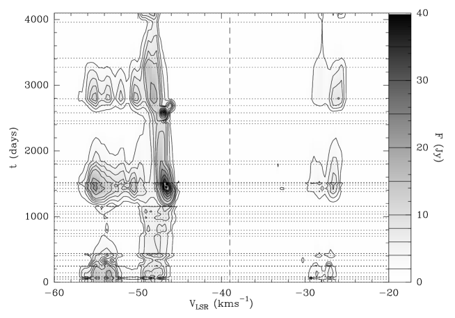
Figure 1.: Grey-scale plot and contour map of the H₂O flux density versus velocity as a function of time for OH83.4$-$0.9. The horizontal dotted lines indicate when a spectrum is available; observations separated by less than 10 days were averaged. Between adjacent observations linear interpolation was performed. Contour values (start(step)end) are 2(2)10(5)40 Jy (black); 45(5)55 Jy (white). The vertical dashed line indicates the stellar velocity; t=0 at JD2447940.

Figure 2.: a. (left) Upper envelope of the H₂O emission (above $5\,\sigma$) of OH83.4$-$0.9. b. (right) Frequency histogram of OH83.4$-$0.9. Shown for each channel is the number of times that the emission reached above the 5 $\sigma$-level during the entire monitoring period. For both panels, the data were resampled to a resolution of 0.33 kms^-1; V_up and V_fr (see text) are indicated.

4. Results

Because of space restrictions, we only list some of the main results of the analysis of 10 stars from our sample.

$\bullet$ The brighter the central star (larger L_bol), the stronger the maser (larger L${}_{H_{2}O}$) (Fig. 3a).

$\bullet$ Stronger masers have more components, and show less variability (Figs. 3b, c). Stronger masers are also characterized by larger mass loss and larger shell size.

$\bullet$ Mass loss rate Ṁ and the size of the circumstellar envelope are correlated. In Miras and SR-variables (smaller Ṁ) the water masers originate from regions relatively close to the star, and have preferentially tangential gain paths; the velocity range of the emission is $\sim 15$ kms^-1. It is roughly twice that for the OH/IR and Supergiant stars (higher Ṁ), where the masers are found at larger distances from the star and radial gain paths dominate. The transition between the two regimes seems to occur at Ṁ $\sim 4\times 10^{-6}$ M_⊙yr^-1 (Fig. 3d).

$\bullet$ Many emission components in the spectra show a change in V_lsr with time. Where blending does not seem to be a problem, values of (de-)acceleration between 0.06 and 0.40 kms^-1yr^-1 are typical; the largest velocity change is found for a flare component in RX Boo: $-$0.4 kms^-1 in 84 days (=$-1.74\pm 0.20$ kms^-1yr^-1).

$\bullet$ For stars where a period could be determined from the maser data, we find that the period of the maser is the same as that of the optical and IR emission. There is however a phase delay ($\sim 0.1-0.3$) for the H₂O maser.

$\bullet$ The emission, integrated over the blue (V$<V_{\ast}$) and red (V$>V_{\ast}$) parts of the spectra, shows the same change with time. The masers in OH/IR stars have radial gain paths, and in these objects the blue part of the emission dominates over the red part. This can be caused by maser amplification of the stellar radio-continuum radiation and/or geometric blocking of the red light by the star (Takaba et al. [2]).

Figure 3.: a. (top left) $\rm L_{H_{2}O}(up)$, the maximum maser luminosity, determined from the upper envelope, as a function of the stellar L_bol b. (top right) The variability index, defined as the ratio between the maximum integrated flux density S_max reached during the observations, and the average flux density $<$S$>$, as a function of $\rm L_{H_{2}O}(up)$ c. (bottom left) The number of emission components in the spectrum with the highest $\rm\int Fd\nu$, as a function of $\rm L_{H_{2}O}(up)$ d. (bottom right) The maximum detected velocity range of the maser emission as a function of the mass loss.

5. What can the SRT do for us?

The arrival of the SRT will both improve the quality of the maser data, and spawn new research projects. A direct consequence of the presence of the SRT will be that we can perform more frequent monitoring of our objects, resulting in a better time-coverage. The higher angular resolution of the SRT will reduce spectral contamination by nearby, unrelated water masers, which can be a problem for masers in star-forming regions. The expected superior quality of the surface of the dish results in higher sensitivity, a cleaner beam, and hence more efficient observations, and the possibility to detect fainter maser components. We should also be able to observe more (faint) calibrators than what is presently possible at Medicina.

During the years of monitoring several flares were found in the maser spectra. The causes for these phenomena are not known, nor is their frequency of occurrence. A systematic patrol, facilitated by the presence of the SRT, of a large sample of bright maser sources, followed by target-of-opportunity observations at the VLA (or VLBA), may result in a better understanding of maser flares.

Models of circumstellar shells have become increasingly complex, and involve non-spherical multiple shells, which are the result of mass loss rates that vary on time-scales of years or even decades. If these variations in mass loss rates are common in late-type stars, one may be able to see the effects also in the water maser properties (e.g. changes in average luminosity, and velocity range of the emission over the years). Continued and frequent monitoring of a large sample of objects is required to reveal these gradual changes, and will help to constrain wind models.

Finally, the detectors planned for the SRT will allow observations of other masers as well, such as those of SiO.

References

- [1] Brand J., Baldacci L., Engels D., 2002, A study of the H2O maser emission from R Cas. In: V. Migenes, E. Lüdke (eds.) Cosmic Masers: from Protostars to Black Holes. IAU Symp. 206 (ASP) in press (astro-ph/0105274)
- [2] Takaba H., Ukita N., Miyaji T., Miyoshi M., 1994, PASJ 46, 629