ESO Imaging Survey

Stellar catalogues in five passbands ($UBVRI$) over an area of approximately 0.3 deg², comprising about 1200 objects, and in seven passbands ($UBVRIJK$) over approximately 0.1 deg², comprising about 400 objects, in the direction of the Chandra Deep Field South are presented. The 90% completeness level of the number counts is reached at approximately $U$ = 23.8, $B$ = 24.0, $V$ = 23.5, $R$ = 23.0, $I$ = 21.0, $J$ = 20.5, $K$ = 19.0. These multi-band catalogues have been produced from publicly available, single passband catalogues. A scheme is presented to select point sources from these catalogues, by combining the SExtractor parameter class_star from all available passbands. Probable QSOs and unresolved galaxies are identified by using the previously developed $\chi^{2}$-technique (Hatziminaoglou et al. 2002), that fits the overall spectral energy distributions to template spectra and determines the best fitting template. Approximately 15% of true galaxies are misclassified as stars by the $\chi^{2}$ method. The number of unresolved galaxies and QSOs identified by the $\chi^{2}$-technique, allows us to estimate that the remaining level of contamination by such objects is at the level of 2.4% of the number of stars. The fraction of missing stars being incorrectly removed as QSOs or unresolved galaxies is estimated to be similar. The observed number counts, colour-magnitude diagrams, colour-colour diagrams and colour distributions are presented and, to judge the quality of the data, compared to simulations based on the predictions of a Galactic Model convolved with the estimated completeness functions and the error model used to describe the photometric errors of the data. By identifying outliers in specific colour-colour diagrams between data and model the level of contamination by QSOs is alternatively estimated to be $\stackrel{{\scriptstyle<}}{{\sim}}$ 6.3% in the seven passband and $\stackrel{{\scriptstyle<}}{{\sim}}$2.3% in the five passband catalogue. This, however, depends on the exact definition of an outlier and the accuracy of the representation of the colours by the simulations. The comparison of the colour-magnitude diagrams, colour-colour diagrams and colour distributions show, in general, a good agreement between observations and models at the level of less than 0.1 mag; the largest discrepancies being a colour shift in $V-R$ and $R-I$ of order of 0.2 mag possibly due to uncertainties in the bolometric corrections. Although no attempt is made to fit the model to the data, a comparison shows that the lognormal law for the initial mass function proposed by Chabrier (2001) describes the data better than the power law form in that paper. The resulting stellar catalogues and the objects identified as likely QSOs and unresolved galaxies with coordinates, observed magnitudes with errors and assigned spectral types by the $\chi^{2}$-technique are presented and are publicly available.

1 Introduction

The primary goal of the ESO Imaging Survey project is to conduct public imaging surveys to provide data sets from which statistical samples of different types as well as of rare population objects can be drawn for follow-up observations with the VLT. A summary of the surveys conducted so far can be found in da Costa et al. (2001). Recently, deep optical/infrared observations of the Chandra Deep Field South (CDF-S) have been completed as part of the ongoing Deep Public Survey (DPS), and the data publicly released (Vandame et al. 2001; Arnouts et al. 2001). In these papers, fully calibrated images and single passband catalogues were presented for $UBVRI$ observations covering an area of 0.3 deg² and for $UBVRIJK$ over a region of 0.1 deg² at the centre of the former area. Even though the angular coverage is still relatively small, the particular combination of depth and solid angle of the complete survey and the uniformity of the multi-band data which will result make it worthwhile to explore the type of objects likely to be sampled by the survey, to devise analysis techniques to identify objects of potential interest and to make a first evaluation of the samples that are likely to emerge when the full survey covering 3 deg², is completed.

The present work is in many ways an extension of that presented in Hatziminaoglou et al. (2002; hereafter H2002) which used a $\chi^{2}$-technique to classify point sources according to spectral type using their multi-band photometric properties, trying to identify special objects such as QSO, White Dwarf (WD) and low mass star candidates.

Here, the question of how to choose an optimum stellar catalogue for statistical studies, either using a single passband or using multi-colour data, is discussed in more detail. Procedures are developed to set the contamination by extended sources below a specified value at the single passband level. To reach fainter magnitude limits the leverage of using multi-colour data is investigated. Finally, to assess to some extent the quality of the final multi-colour stellar catalogue produced, number counts, colour distribution, and colour-colour and colour-magnitude diagrams are compared to those predicted by a Galactic model calibrated using independent data.

In Section 2 the data are briefly reviewed as well as the method employed in the construction of the point source catalogue used in the present paper. Section 3 discusses how point sources are selected in the single passband, and colour catalogues, and how potential unresolved galaxies and QSOs are found using a previously developed $\chi^{2}$-technique. In Section 4 the actual procedure for the creation of the single passband to the final stellar colour catalogue is presented. Section 5 and Section 6 introduce the Galactic Model and the simulation of appropriate data sets. Section 7 presents the results. Finally, in Section 8 a brief summary is presented.

2 The data

The single passband catalogues for the CDF-S are taken from Vandame et al. (2001) and Arnouts et al. (2001), cut at a $S/N=2$, slightly lower than the catalogues publicly released which were cut at a $S/N=3$.

This is done as a magnitude, even with a larger error bar, is preferred over an upper limit which would otherwise be assigned to the magnitude in a filter where an object is not detected.

The $U$-band catalogue used here (and in H2002) was extracted from an image produced by stacking all the available $U/38$ and $U350/60$ images, to reach a fainter limiting magnitude. A more detailed discussion of this catalogue and of its photometric calibration will be present in Arnouts et al. (in preparation). The main conclusion is that a shift of +0.2 mag has to be applied to the $U$-magnitudes given by SExtractor running on the stacked $U$ image using the photometric zero point of the $U/38$ image, to get agreement between observed and predicted $U-B$ colours for normal stars.

To build a colour catalogue, the single passband catalogues are associated on position using, in the present paper, a fixed search radius of 0.8″. With this search radius the number of multiple associated sources is kept low ($\stackrel{{\scriptstyle<}}{{\sim}}$0.8% in all passbands, and typically 0.2%), while resulting in many positive matches. A detailed discussion on the optimum search radius, and more complicated schemes using variable search radii will be presented elsewhere (Benoist et al. 2002).

After the association, only objects that are in the area common to all catalogues and outside all the masks placed around saturated objects and bright stars are kept. This ensures that all objects could, at least in principle, have been detected in all passbands. The effective area is 0.263 deg² for the five passband catalogue and 0.0927 deg² for the seven passband catalogue. If an object is not associated in a passband, an 3$\sigma$ upper limit is assigned for the magnitude in that passband.

3 Selecting Point Sources

3.1 Selecting Point Sources at the single passband level

The SExtractor software package used at the moment to detect and extract sources uses a neural network to separate point from extended sources. For each object it returns a parameter, class_star, with a value between 1 (a perfect point like object) and 0. An example of the distribution of class_star as a function of magnitude is shown in Fig. 1 for the $R$-band.

The neural network file used here is the standard one that is part of the SExtractor package and that has been trained for seeing FWHM values from 0.025 to 5.5″ and for images that have 1.5 $<$ FWHM $<$ 5 pixels, and is optimised for Moffat profiles with 2$\leq\beta\leq$ 4. These conditions are fulfilled for the EIS optical and IR observations of the CDF-S.

At the bright end of the distribution shown in Fig. 1 two sequences can easily be distinguished with class_star values below 0.1 and above 0.95, respectively. However, for fainter magnitudes the sequences spread out and merge. In previous EIS papers (e.g. Prandoni et al. 1999) the notion of a morphological classification limit mag_star_lim was introduced, where objects brighter than this limit and with a class_star value larger than a limit class_star_lim were considered point sources. In previous papers, these limits were chosen basically by eye from figures like Fig. 1.

Figure 1: SExtractor parameter class_star versus magnitude for the $R$-band, with the finally adopted morphological classification limits indicated by the solid line. Objects in the upper left box are considered point sources in a single passband. The dashed line indicates the much simpler criterion used previously which only took into account the class_star value at the faintest mag_star_lim.

Clearly, there is a need to determine class_star_lim and mag_star_lim in a more systematic way, by statistically describing the relative contribution of the point- and extended-source population. The goal is to produce a magnitude-dependent classification as illustrated in Fig. 1.

A technical description of the actual implementation of the concept used in the present paper is given in the Appendix, and Fig. 1 shows for the $R$-band the distribution over class_star and the adopted values for class_star_lim and mag_star_lim (solid line) in the present paper and for comparison the old way of using a single value (dashed line). It should be noted that this procedure allows the estimate of the smallest class_star where stars can be distinguished over the large background of galaxies. It does not imply, especially at the faint end, that stars with class_star values lower than class_star_lim do not exist. Furthermore, it is recalled that the actual distribution of class_star versus magnitude depends on the seeing but also on the Galactic coordinates of the field under consideration.

It is important to emphasise that more work should be done to explore alternative ways of morphologically classifying images. One alternative under consideration is to use multi-resolution methods to provide an independent pixel-based classification scheme (Vandame, private communication).

Apart from a statistical analysis of the distribution of class_star versus magnitude a second criterion of selecting point sources is investigated, namely the fact that they are expected to be “round”. This is done by considering the SExtractor parameters $A$ and $B$ which represent the profile fitting rms along the major and minor axis (see Arnouts et al. 2001 for more discussion). Visual inspection of some objects with large values of $\mid(A-B)/(A+B)\mid$ showed that these outliers are not stellar, but bad pixels, or objects close to the edge of a frame or a mask. The standard deviation of the distribution is computed and objects that deviate by more than a specified level (in the present paper 6$\sigma$) are not considered point sources. Typically, 0.1% of the objects are removed in this way. A 3$\sigma$ clipping, however was verified to be too stringent, as then many true stars would be removed. Most of them would be recovered by the colour Point/Extended (hereafter, P/E) source classification scheme discussed below, but they would, incorrectly, be excluded from the single passband number counts.

3.2 Selecting Point Sources in a colour catalogue

The (P/E) source classification in a colour catalogue is a non trivial matter, as the mag_star_lim and class_star_lim of all the passbands involved must be combined in some way. Here the following scheme is adopted. As the (P/E) source classification is most reliable for bright objects (see Fig. 1), the classification in the colour catalogue will be determined by the passband in which the object is brightest relative to the (faintest) mag_star_lim in that passband. If the object is classified as a point source in this passband, it is considered a point source in the colour catalogue. The fact that the seeing in the images is different is implicitly taken into account by the fact that the mag_star_lim in a case of worse seeing is brighter than in the case of good seeing.

A completely different way of creating a colour catalogue is by digitally stacking the images in the various filters, and then running the source detection algorithm on it. The photometry is then obtained by going back to the individual filters and measure the flux around the now known positions. This method was applied to EIS data by da Costa (1998) using the algorithm of Szalay et al. (1999). From that work, SExtractor’s standard neural network for (P/E) source classification is known not work properly on such a stacked image because of e.g. seeing variations among the different filters. Therefore this procedure is not further pursued here.

3.3 Eliminating non-stellar objects

The procedures outlined above can only separate point-like from extended objects. However, to produce a truly stellar catalogue one has to consider the possibility of contamination by QSOs and unresolved galaxies. This is not possible in a single passband catalogue. However, in a multi-colour catalogue the photometric data provides information on the shape of the Spectral Energy Distribution (SED) which can, in principle, be used to address this issue.

In fact, this was the subject of the paper of H2002 where a colour point source catalogue was used to classify sources according to their spectral type. This was done by $\chi^{2}$-fitting template spectra to the observed magnitudes in different bands. The spectral library in use consists of series of: model QSO, WD and brown dwarf spectra; three empirical cool WD spectra; a set of stellar templates for O-M stars; and a set of model galaxy spectra. In H2002 emphasis was given in identifying QSOs, WD and low mass star candidates for follow-up spectroscopy. The $\chi^{2}$-technique provides an independent view of the nature of a source, complementing the morphological classification. However, by using broadband photometric data to assign spectral types, misclassifications are possible (e.g. due to the fact that an object is an unresolved binary leading to composite colours) and this is further discussed in Sect. 7.5.

3.4 Choosing parameters

The morphological classification limits adopted in the present paper are listed in Tab. 1 and are chosen after extensive testing. In terms of the technical description in the Appendix the parameter $t_{2}$ is set to 30 and the parameter $t_{1}$ to 80.

The main guideline to chose these particular values for $t_{1}$ and $t_{2}$ to set the mag_star_lim and class_star_lim values is the estimate of the remaining contamination by QSOs and unresolved galaxies, and related, the incorrect removal of true stars by misclassification of the $\chi^{2}$-technique, which one wants to keep small (of order a few percent at most). These numbers are estimated independently in Sects. 7.2.2 and 7.5.

Table 1: Morphological classification limits mag_star_lim ($m_{\rm x}$) and class_star_lim ($c_{\rm x}$) adopted in the single passband catalogues (see Fig. 8 for a visual representation).

Passband	$c_{1}$	$m_{1}$	$c_{2}$	$m_{2}$	$c_{3}$	$m_{3}$	$c_{4}$	$m_{4}$
$U$			0.851	21.57	0.873	22.27	0.952	22.45
$B$			0.848	23.04	0.933	23.75	0.961	23.84
$V$	0.590	21.15	0.828	22.15	0.879	22.68	0.935	22.69
$R$	0.863	20.98	0.873	21.89	0.907	22.41	0.915	22.61
$I$	0.603	19.30	0.663	20.25	0.744	20.77	0.885	21.09
$J$			0.644	19.32	0.929	20.18	0.923	20.36
$K$					0.750	17.71	0.943	18.46

Table 2: Number of objects in the five and seven passband point source catalogues

	$UBVRI$
Number of point sources	1371
Passband that decided (UBVRI)	7/308/0/650/406
Not classified by $\chi^{2}$ method	18
Classified by $\chi^{2}$ method	1353
as rank 1	947
as rank 2	127
as rank 3	279
Number of unresolved galaxies	37
Number of QSOs	136
Number of stars	1198
	$UBVRIJK$
Number of point sources	486
Passband that decided (UBVRIJK)	2/110/0/225/37/110/2
Not classified by $\chi^{2}$ method	5
Classified by $\chi^{2}$ method	481
as rank 1	160
as rank 2	117
as rank 3	204
Number of unresolved galaxies	16
Number of QSOs	61
Number of stars	409

4 The procedure

For the chosen combination of class_star_lim and mag_star_lim, the single passband catalogues are produced and then associated to form the colour catalogue with the (P/E) source classification applied based on all the available colours. This is done separately for the $UBVRI$ and $UBVRIJK$ catalogues. The resulting number of point sources is given as the first entry in Table 2. The second entry gives the split over the passband that actually decided that a source is considered a point source. In the five passband catalogue this is mainly $R$, $I$ and $B$; in seven passbands mainly $R$, $J$ and $B$.

As a second step the $\chi^{2}$ template fitting of H2002 is applied to the objects classified as point sources. This is done twice: once with and once without the galaxy template spectra included. The outcome of the template fitting is the spectral type of the best fitting template spectrum (with associated photometric redshift in the case of QSOs and galaxies), the (reduced) $\chi^{2}$ and the “rank” (which is based on the $\chi^{2}$ value, rank 1 being the robust candidates, rank 3 poor candidates). Objects that are ranked 3 when no galaxy templates are considered (typically having reduced $\chi^{2}$ larger than 4-7), and become ranked 1 galaxies when galaxy templates are considered, that are fainter than 16th magnitude (in the passband where they are brightest) and with photometric redshifts larger than 0.25 are considered to be (unresolved) galaxies and are removed from the list of point sources. The split over the assigned ranks, the number of unresolved galaxies and QSO, and the number of objects considered true stars are given in Table 2.

The $\chi^{2}$-technique requires an object to be detected in at least three passbands. Less than 1.5% of objects does not fulfil this criterion (see the third entry in Tab. 2). They are kept as stars, as they are originally classified as point sources and there is no evidence to the contrary. Exclusion of this small number of objects does not affect any of the conclusions of this paper.

From an observational point of view, the validity of the adopted approach to remove the most likely galaxy and QSO interlopers can be verified only by spectroscopic follow-up of a representative sample of objects. From a theoretical point of view it is planned in the future to simulate the physical size, redshift and colour space occupied by galaxies and QSOs as well, so it can be verified if a unresolved source within a given colour bin is more likely to be a star, galaxy or a QSO.

The final number of objects considered to be stars is about 1200 over the 0.263 deg² for the five passband catalogue and about 400 over the 0.0927 deg² for the seven passband catalogue. For comparison, the number of extended objects over these areas is about 74000 and 28000, respectively.

5 The Galactic model

The observed counts and colours will be compared to a newly developed Galactic model (Girardi et al. in preparation). In brief, this model is based on a population synthesis approach, where stars are randomly generated from an extended library of evolutionary tracks according to user defined star formation rate (SFR), age-metallicity relation (AMR), and initial mass function (IMF), and then distributed in space according to the probabilities given by the specified geometry. The evolutionary tracks include brown dwarfs down to 0.01 M_⊙, and evolved phases with the complete white dwarf stage for stars up to 7 M_⊙. For the present paper the following ingredients have been adopted:

• The IMF is taken to be the lognormal form proposed by Chabrier (2001). The effect of adopting the power law form proposed by him will be detailed in Sect. 7.1.4

• The SFR is assumed to be constant over the last 11 Gyr for the disk, and constant between 12 and 13 Gyr for the halo.

• The AMR for the disk is taken from Rocha-Pinto et al. (2000). [Fe/H] values are converted into the metal content $Z$ by means of a relation that allows for $\alpha$-enhancement at decreasing [Fe/H], as suggested by Fuhrmann (1998) data. At any age, [Fe/H] is assumed to have a 1$\sigma$ dispersion of 0.2 dex.

  The metallicity of the halo stars is assumed be $Z$ = 0.0095, with a dispersion of 1.0 dex. This is based on an observed [Fe/H] value of $-1.6\pm 1.0$ (Henry & Worthey 1999), allowing for an $\alpha$-enhancement of 0.3 dex.

• The disc component is described by a double-exponential in scale height and Galactocentric distance. The model does not have separate components for thin or thick disk. Instead the scale height for disk stars is a function of age, and is parameterised as:

  $$H=z_{0}\;\;(1+t/t_{0})^{\alpha}$$ (1)

  with $t$ the age of the star. Rana & Basu (1992) for example find $z_{0}$ = 95 pc, $t_{0}$ = 0.5 Gyr and $\alpha$ = (2/3). However this does not fit very well the derived scale height of ‘thick’, ‘old’, ‘intermediate’ and ‘young’ disk components as derived by Ng et al. (1997). Their results are described by $z_{0}$ = 95 pc, $t_{0}$ = 4.4 Gyr and $\alpha$ = 1.66, which are adopted here.

For the present paper the (relative) local densities of halo and disk stars, the oblateness of the halo and the Galactocentric disc scale length are derived from the “Deep Multicolor Survey” (DMS; Osmer et al. 1998 and references therein) covering six fields and EIS data (Prandoni et al. 1999) for the South Galactic Pole. A more detailed discussion of the calibration of the Galactic model will be given in Girardi et al. (in preparation). Note that the Galactic model parameters derived below differ slightly from those used by H2002 to compare some of their results to.

The halo oblateness (and local halo number density) is derived by fitting the number of halo stars, defined by (in the Johnson-Cousins system) $0<B-V<0.7$ in the range $20<B<22$ and $0<V-I<0.8$ in the range $18<I<20$, in these seven fields and is found to be $q=0.65\pm 0.05$. This value is smaller than the value of 0.8 $\pm$ 0.05 quoted by Reid & Majewski (1993), but recently Robin et al. (2000) could not exclude a spheroid with a flattening as small as $q=0.6$ and Chen et al. (2001) derived $q=0.55\pm 0.06$.

The disc radial scale length (and local disk number density) is derived by fitting the number of disk stars, defined by $1.3<B-V<2.0$ in the range $20<B<22$ and $1.8<V-I<4.0$ in the range $18<I<20$, and is found to be $H_{\rm R}=2800\pm 250$ pc. This is in agreement with the lower limit of 2.5 kpc (Bahcall & Soneira 1984) and the recent work of Zheng et al. (2001) on M-dwarfs who derive $H_{\rm R}=2750\pm 160$ pc and Ojha (2001) who derive $H_{\rm R}=2800\pm 300$ pc for the thin disc.

The model with these parameters is applied to the CDF-S field. The Galactic bulge has no contribution in this direction. The model is calculated for an area of 3 deg², which is about 10 times larger than the actual area covered by the $UBVRI$ data, and about 30 times larger than the area covered by the $UBVRIJK$ observations. This ensures that the parameter space is properly sampled and that the errors on the model data are at least 3, respectively 5, times smaller than the error bars on the observed data.

6 Simulations of the observed data

The galactic model produces “perfect” stellar objects down to a specified magnitude (in fact the model is computed down to $R$ = 30.5). To build a mock colour catalogue simulating the real data, the magnitudes from the galactic model are taken as input and the following steps are considered:

• The error in the magnitude (as computed by SExtractor) as a function of magnitude for each band (based on the properties of the actual image and real data). Additionally, one can scale these errors by a factor and add in quadrature an “external error”, simulating for example errors in the photometric zero point. The “observed” magnitude is then drawn from a Gaussian with the estimated error as width and centred around the “perfect” magnitude. The scaling factor and “external error” used in the present paper are given below.

• The saturation at bright magnitudes. The ADU level in the central pixel of an object is simulated, and compared to the actual value used by SExtractor to flag a saturated object.

• The completeness at the faint end. Artificial star tests using the EIS images themselves have not yet been performed to estimate the completeness functions. As a temporary solution the completeness functions have been derived for the $R$-band and $K$-band by comparing the EIS data to the deeper observations of respectively Wolf et al. (2001) and Saracco et al. (2001) over the parts where their observations overlap with the EIS observations. For the other bands the shape of the function that describes the completeness is kept the same (for $UBVI$ taking $R$ as a reference, and for $J$ taking $K$ as the reference), and scaling the characteristic magnitude where the incompleteness sets in using the 5$\sigma$ limiting magnitude of the bands as a reference. For the stellar catalogue considered here the exact details of the completeness functions are not of too much importance as the estimated magnitudes where the EIS data is estimated to be 50% complete ($U$ = 25.1, $B$ = 26.6, $V$ = 25.5, $R$ = 25.4, $I$ = 24.3, $J$ = 22.9, $K$ = 21.2) are at the very faint end of the stellar catalogue. In other words, the depth of the stellar catalogue is set by the ability to separate point from extended sources and the remaining contamination by QSOs and unresolved galaxies, not the depth or incompleteness of the observations as such.
  These same observations are used to compare the differences in the magnitudes of the objects in common between EIS and the external data. Slices in magnitudes are made, and the average error for the EIS observations, the average error for the comparison catalogue (hence Wolf et al. for $R$, and Saracco et al. for $K$), and the rms of the difference of the stars in common determined. The errors in the external catalogues are always smaller than in the EIS data, as expected since these observations are deeper than ours. However, both underestimate the error as compared to the rms in the difference. Based on these comparisons an external error of 0.01 mag in $UBVRI$ and 0.03 mag in $JK$, and a scaling factor of two in all passbands are adopted in the simulation of the errors. With this description the width of the stellar sequence in the colour-colour diagrams is described extremely well for all magnitudes and passbands (see Fig. 4).

The simulation also takes into account the S/N limits imposed on the single passband and colour catalogues. Furthermore, objects that are saturated in one or more bands are removed from the mock catalogue, as masks are placed around them in the real data and only objects outside all masks are being considered in the final colour catalogue.

Finally, two types of mock stellar catalogues are produced. One considering all simulated point sources that are potentially “observable”, and the second catalogue that also takes into account the way that point sources are being selected from the real colour catalogue by checking if the object is brighter than the morphological classification limit used in the production of the observed data set in at least one passband (see Tab. 1). This is a conservative estimate, as for the real data the value of the SExtractor parameter class_star also plays a role. However this feature in fact allows us to check if the class_star values chosen are not too low (resulting in too many galaxies and leading to high stellar number counts at the faint end) or too conservative (leading to number counts that are below the predictions). Details on the simulation of the photometric errors, the completeness model and the simulated datasets will be given elsewhere (Groenewegen et al. 2002, in preparation).

7 Results and analysis

In this section the observed number counts, colour-colour and colour-magnitude diagrams, and colour-distribution histograms are presented and compared to the simulations. The effectiveness of using the $\chi^{2}$-technique is discussed. Finally, catalogues of stellar sources, QSOs, and unresolved galaxies are presented. Due to space constraints only representative figures will be shown and the full set of figures is only available through the on-line edition of A&A. Note that most of the figures need to be viewed or printed in colour.

7.1 Number counts

7.1.1 General description

Figure 2 shows the number counts for every passband from the five passband catalogue for $UBVRI$ and from the seven passband catalogue for $JK$. In the lower right panel the $R$-band number counts are shown based on the seven passband catalogue. The agreement with that from the five passband catalogue is excellent, and the same applies when comparing the number counts in the other optical bands as derived from the five and seven passband catalogues.

In the left-hand panels the predictions by the galactic model are shown, namely the contributions by the disk (dashed and solid thin black histograms), the halo (dashed and solid blue histogram) and their sum (dashed and solid thick black histogram). Shown are the predictions from the “perfect” model (the blue and black dashed histograms), and the predictions taking into account the error model, saturation, completeness and the mag_star_lim limits that are used to create the colour catalogue (the blue and black full histograms). The left-hand panels illustrate the relative contributions of disk and halo at various magnitudes. In this particular field the contribution of the disk exceeds that of the halo for almost all observed magnitudes. The model predicts, however, that obtaining deeper images and assuming one would be able to do the (P/E) classification at the level of $J,K\approx 23-24$ the number counts should be dominated by the halo. In the optical the halo dominates the disk only at much fainter magnitudes ($I\approx 25$, $V\approx 28$). Deeper infrared data could therefore better constrain the IMF and other parameters describing the halo than the present data.

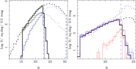
Figure 2: Number counts in $UBVRI$ from the five passband catalogue and in $JK$ from the seven passband catalogue. This sample is for the $R$-band, and the full figure is only available in the on-line edition. In the lower right panel the $R$-band counts based on the seven passband catalogue are presented. They are in good agreement with those based on the five passband catalogue, as is the case for $UBVI$. Left panel: shown are the disk component (dashed and solid thin black histograms) and halo component (dashed and solid blue histograms), and their sum (dashed and solid thick black histograms) predicted by the galactic model. Distinguished are the predicted model counts taking into account the error model, saturation, completeness and the mag_star_lim in the individual passbands (the blue and black full histograms), as well as the “perfect” model (the blue and black dashed histograms). The morphological classification limits for the bands are indicated by the vertical dashed line. Right panel: comparison of the data (blue coloured histogram with errors bars) with the model. Note the different magnitude scale w.r.t. the left-hand panel. Shown are the predicted counts taking into account the error model, saturation and completeness (thick dotted black line), as well as the counts that additionally take into account the mag_star_lim limits in the individual passbands (thick solid black line; the same curve as in the left-hand panel). The pink histogram represents the observed number counts using the point source classification for that band only. The number counts of objects assigned “stellar” template spectra that are ranked 1 and $\leq 3$ in the full five and full seven passband catalogue respectively, based on the $\chi^{2}$-technique only, are indicated by the dashed blue histogram. The QSO numbers counts (among the objects initially classified as point sources) are indicated by the red histogram. The morphological classification limits for the bands are indicated by the vertical dashed line.

In the right-hand panels, the model predictions (again, the full thick black histogram) are compared to various datasets. The blue histogram with the error bars (based on $\sqrt{N}$ statistics) represents the observed stellar number counts from the colour catalogue based on the (P/E) classification and subsequent application of the $\chi^{2}$-technique described in Sect. 4. The pink histogram represents the number counts using the (P/E) classification for that band only. As, by construction, there are no stars fainter than mag_star_lim in the single passband catalogue, but this value usually does not coincide with the borders of the binning, the counts in the last bin may drop artificially. Therefore, the counts in the last bin of the pink histogram are corrected for this effect by multiplying the counts in the last bin by the bin width divided by the actual width over which there is data.

7.1.2 Comparing counts from single passband and colour catalogues

Up to mag_star_lim, indicated by the vertical dashed line, the counts from the single passband and the colour catalogue are in very good agreement. In fact, naively, one might even have expected them to be identical. They are not for several reasons.

Firstly, in particular in $U$, at the bright end, the counts from the single passband are above the counts from the colour catalogue. This is due to the fact that only objects which are outside all masks created at the single passband level are considered in the colour catalogue. Since the $U$-band is shallow, the single passband catalogue contains objects that are not saturated in $U$, but are saturated (hence will have a mask placed around them) in one of the other bands, and will not make it into the colour catalogue.

Secondly, the “good” area over which the sources are considered is slightly larger for the single passband catalogues compared to the colour catalogue, as the different single passband images do not exactly have the same field centre and the colour catalogue is created over the area that is in common to all passbands. At bright and intermediate magnitudes the counts match to within the Poisson errors, as expected (except for the $U$-band for reasons just discussed).

Thirdly, when approaching the morphological classification limit the number counts based on the colour catalogue tend to fall below the counts based on the single passband. This is due to the fact that galaxy interlopers and QSOs have been removed from the sample using the $\chi^{2}$-technique applied to the objects detected in three or more passbands. As illustration, the QSO number counts for the objects originally classified as point sources is shown by the red histogram.

Beyond the morphological classification limit, the number counts based on the single passband level drop to zero (by construction), while the number counts based on the colour catalogue extend to significantly fainter magnitudes. This illustrates the usefulness of using all available colours to construct a point source catalogue. This is especially true in $U$, where the counts reach almost two magnitudes fainter than the single passband counts. This is because the $U$ data is shallow compared to those in the other bands and most of the information on the (P/E) classification comes from redder passbands. The gain in magnitude is negligible in $R$ which, according to Tab. 2, in most cases defines the (P/E) classification.

7.1.3 Comparison with the model and literature

The counts predicted by the model and the observations from the colour catalogue are in good agreement, considering that no fine tuning or fitting was performed. The observed data follow the thick black lines within the errors indicating that the choice of class_star is appropriate (or at least consistent with that predicted by the model). The data fall below the dashed thick lines, which would be the predicted counts if the (P/E) classification would be reliable for all magnitudes. Based on the flattening of the observed counts and guided by the results from the model the 90% completeness limits are estimated to be approximately $U$ = 23.8, $B$ = 24.0, $V$ = 23.5, $R$ = 23.0, $I$ = 21.0, $J$ = 20.5, $K$ = 19.0.

The deepest stellar counts available in the literature are from the hst, but they cover a small area, e.g. Santiago et al. (1996) combine 17 WFPC-2 fields for a total area of 0.027 deg², 90% complete to $I_{814}$ of 22 to 24 depending on the field. At the other end of the spectrum there is the recent analysis of Chen et al. (2001) using 279 deg² of sdss data complete to a depth of $g^{\prime}$ = 21.0 (corresponding to approximately $V$ = 20.4 for a typical colour of $g^{\prime}-r^{\prime}$ of 1, or three magnitudes brighter than ours), or Ojha (2001) that analyse seven fields of 2mass data covering 67 deg² down to $K_{\rm s}$ = 15. Intermediate large area surveys are e.g. the “Deep Multicolor Survey” (DMS; Osmer et al. 1998 and references therein) covering six fields of about 0.14 deg² each complete to about $B$ = 23.5 (comparable to ours), or Reid & Majewski (1993) covering 0.3 deg² complete to about $V$ = 21.5 (brighter by two magnitudes compared to ours).

What will make the DPS survey unique when finished is that it will cover a larger area, to a depth that is comparable or better, than existing intermediate large area stellar surveys and that the data will be in five or seven passbands.

7.1.4 The slope of the IMF

In this Section the influence of the shape of the IMF on the number counts is illustrated. Figure 3 shows the number counts in $R$ and $J$ when the power law form in Chabrier (2001) is adopted instead of his lognormal law. The number counts at $R\sim 22$ and $J\sim 19-20$ are larger than in the default case by about 20%. In the other bands the effect is less striking but also present. This illustrates the potential of the present data, especially when the DPS survey is completed and data of similar depth on fields with different galactic coordinates are available, to constrain e.g. the IMF. The counts in this field are better fitted with the lognormal law proposed by Chabrier (2001) than the power law proposed by him. The stars in the relevant magnitude interval have typical masses of about 0.1 - 0.2 M_⊙. However, the fits are certainly not perfect, and this possibly hints to a more complex, or different, shape of the IMF than a power law or lognormal law.

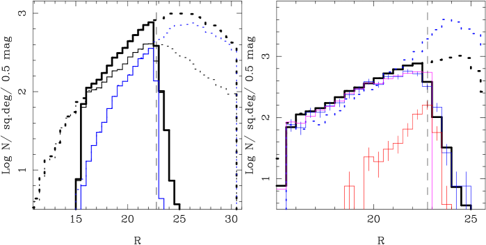
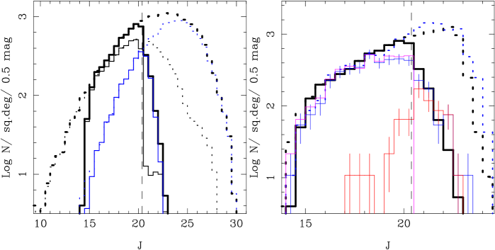
Figure 3: Number counts in $RJ$ with the power law form of the IMF from Chabrier (2001). The meaning of the curves is as in Fig. 2. The counts at $R\sim 22$, $J\sim 19.5$ are about 20% larger than for the standard case with the lognormal form.

7.2 Colour-colour diagrams

7.2.1 General description

Figure 4 shows selected colour-colour diagrams split into magnitude bins for the five and seven passband catalogues. In the left-hand panel the predictions by the model are shown. Objects from the halo (open circles) and the disk (filled circles), with stars with $\log g>7$ (representing WDs) and stars with masses $<$0.1 M_⊙ (representing low mass stars) additionally marked by a plus and cross sign, respectively. The right-hand panel shows the stellar objects (filled and open circles), while the objects identified as QSOs by the $\chi^{2}$-technique are shown as crosses.

The overall agreement is very good in all cases and for all magnitude bins. In particular the width of the sequences is well matched to the data confirming a-posteriori the correctness of scaling the simulated errors by SExtractor as was derived by the comparison to deeper external data.

The largest discrepancies are: (a) in the $(V-R)-(R-I)$ diagram, where for increasing $R-I$ the model predictions saturate at a level of $V-R$ of $\sim 1$, while the observed data points continue to become redder; (b) in the $(R-I)-(I-J)$ diagram, where the slope of the data and the model differ for $I-J\raisebox{-3.1298pt}{$\stackrel{{\scriptstyle>}}{{\sim}}$}0.8$; (c) in the $(V-J)-(J-K)$ diagram, where for $V-J>3$ the data seem to remain at a constant colour, while there is a slope in the model predictions. Possible reasons for the discrepancies are discussed in Sect. 7.4.2.

7.2.2 Outliers

Obviously there are also outliers in the colour-colour diagrams on the data side. These can be real (for example due to variability) or hint to problems in the catalogue production. This issue is extensively discussed in H2002. Most important for the present paper is to remind that these outliers do not influence the assignment of the spectral type as this is based on all available magnitudes and errors.

To guide the eye, outliers are marked by the open circles. Outliers are defined in the present paper as follows. An imaginary box in colour space is drawn around all of the model stars in the left-hand panel, for each magnitude bin. An object is defined an outlier if an observed data point on the right is not within any of these boxes. The width of the box was set after some experimentation to be 15-30% of the maximum of the range in both colours axis in a given magnitude bin.

This concept is found useful to estimate the possible level of remaining contamination by QSOs and unresolved galaxies that have not been identified as such by the $\chi^{2}$-technique. Although the outliers are marked in all colour-colour diagrams, the diagrams where QSOs are most easily identified based on their difference in colours with respect to normal stars are $(U-B)-(B-V)$ in five passbands and $(U-B)-(B-V)$, $(B-V)-(V-K)$, $(V-J)-(J-K)$ in seven passbands (H2002). Note, however, that the colour-colour diagrams indicate that QSOs and stars overlap in colour-colour space, and therefore no selection based purely on colour-colour diagrams can be made (see also H2002).

The number of outliers in the $(U-B)-(B-V)$ colour-colour diagram in five passbands is 36, 28 of which are in the region occupied by QSOs, while in the $(U-B)-(B-V)$, $(B-V)-(V-K)$, $(V-J)-(J-K)$ colour-colour diagrams in seven passbands there are 63 outliers, 26 of which are in the region occupied by QSOs. However since stars do overlap with QSOs it can not be assumed automatically that all outliers are QSOs. The upper limits to the remaining contamination by QSOs are therefore $<$6.3% in the seven and $<$2.3% in the five passband catalogue. In Sect. 7.5 an independent estimate of this contamination is given.

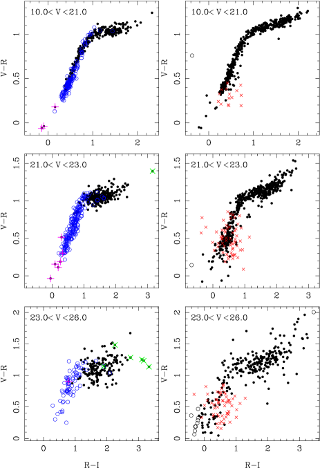
Figure 4: Colour-colour diagram for different cuts in magnitude. This $(V-R)-(R-I)$ diagram based on the five passband catalogue is a typical example and the full figure is only available through the on-line edition. Left panel: Model predictions. Halo (open circles) and disk (filled circles), with stars with $\log g>7$ (representing WDs) and stars with masses $<$0.1 M_⊙ (representing low mass stars) additionally marked by a plus and cross sign, respectively. Since the full simulation is run over $n-$times the observed area, only $\frac{1}{n}$ of all model data points are plotted. Right panel: the data. Open circles represent outliers, in the sense that they are not within a certain magnitude difference of any of the model data points in the left-hand panel (see text). Red crosses are objects identified as QSOs by the $\chi^{2}$-technique.

7.3 Colour-magnitude diagrams

Figure 5 shows selected colour-magnitude diagrams. In the left-hand panel the model predictions are shown with symbols as introduced in Fig. 4. The right-hand panel shows the data. The match is good, in particular the Galactic halo (with bluer colours) and the Galactic disk (with redder colours) are readily distinguished.

One can also notice the particular position occupied by the model very low-mass stars (crosses), that are the reddest and faintest objects in most plots. White dwarfs (plus signs), although found over a relatively wide range of colours and magnitudes, are the only objects to occupy a vertical strip to the blue of the bulk of halo stars: in fact, in diagrams like $V$ vs. $V-R$ and $I$ vs. $V-I$, the sequence of hot WDs (with $V-R<0.3$, $V-I<0.4$) starts at $V\geq 20$ and $I\geq 20$, and this matches quite well the sequence of hot objects seen in the observational plots.

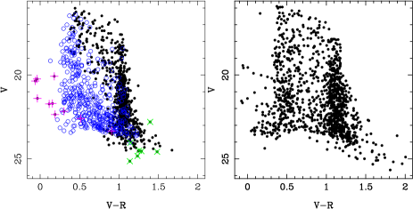
Figure 5: Colour-magnitude diagram. This ($V,V-R$) diagram based on the five passband catalogue is a typical example and the full figure is only available through the on-line edition. Left panel: model results. The symbols have the same meaning as in Fig. 4. Since the full simulation is run over $n-$times the observed area, only $\frac{1}{n}$ of all model data points are plotted. The right panel shows the data.

7.4 Colour distribution

7.4.1 General description

Although the colour-colour and colour-magnitude diagrams provide useful and complementary information, the most stringent test for the comparison between data and model is provided by the distributions over colour at different magnitude slices, as provided in Figure 6.

The overall agreement is again very good. The shape of the colour distributions is correctly recovered in most cases; the absolute number of objects in the faintest bin, however, is not always exact (e.g. $U-B$ and $R-I$).

The most obvious discrepancies are: (a) the excess of objects with $-1<U-B<-0.5$ and $22<U<24$ which could be QSOs not identified by the $\chi^{2}$-technique, or WDs not predicted by the model; (b) the fact that for disk stars the predicted $V-R$ colours are bluer than the observed ones; (c) similarly, that for disk stars the predicted $R-I$ colours are bluer than the observed ones; (d) the excess of observed sources with $J-K>1.2$ and $18<K<19$ which again could be QSOs, or galaxies, not identified by the $\chi^{2}$-technique.

The shifts in colour seen in $V-R$ and $R-I$ are of the order 0.2 mag, but the conclusion is that all the other colours are correctly predicted at a level $\raisebox{-3.1298pt}{$\stackrel{{\scriptstyle<}}{{\sim}}$}0.1$ mag.

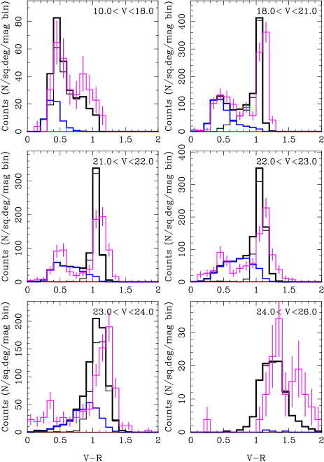
Figure 6: Colour distributions for different cuts in magnitude. The full figure is only available through the on-line edition. Shown are the model predictions (the halo is the blue lined histogram; the disk the thin lined histogram, and their sum is the thick lined histogram) and the data (the pink histogram with the error bars).

7.4.2 Further investigation of the model data

To make better use of the simulations a numerical code has been developed that allows to search on any combinations of the parameters provided by the Galactic Model convolved with the error model, completeness, etc, as described earlier. The parameters provided are the colours with their errors, the Galactic component (i.e. disk, halo, bulge), age, [Fe/H], initial mass, luminosity, effective temperature, $\log g$, distance modulus, visual extinction and apparent bolometric magnitude. Constraints on the differences between two columns are allowed for as well. As an illustrative example the problem of the discrepancy between model and data in the $(V-R)-(R-I)$ colour-colour diagram is addressed. Figure 7 shows the distribution over various model parameters of all simulated stars that are formed in the disc and fulfil $1.4<R-I<3.5$ and $23<R<26$. From this analysis it is clear that mainly low mass stars ($\stackrel{{\scriptstyle<}}{{\sim}}$ 0.2 M_⊙) are contributing to this colour range indicating that likely the theoretical colours for these stars are off by approximately 0.2 mag.

It should be pointed out that, among the possible inadequacies of the model, systematic shifts in the model effective temperatures or in the adopted stellar metallicities would affect all colours in more or less the same way, which does not seem to be the case here. In fact, just a few of the colours are deviant, and this might be related to the tables of bolometric corrections which are adopted in the model. For instance, either these bolometric corrections were derived from imperfect response curves for some of the EIS filters, or the synthetic stellar spectra in use (see Girardi et al. 2002 for details) present inadequacies in some of their wavelength regions (caused by e.g. incomplete line opacity tables). This matter will be further investigated, but whatever is their cause, these colour problems are small enough to not affect any of our conclusions.

Alternatively, these discrepancies may result from the data rather than the model. It is important to point out that most of the discrepancies occur at the near-infrared passbands ($IJK$) where the data may be affected by fringing as well as other problems related to the reduction of jittered infrared data. It will be of interest to see if these problems persist as the techniques for reducing WFI and SOFI data are improved.

Figure 7: Distributions over various parameters of all model stars which are formed in the disc and have $1.4<R-I<3.5$ and $23<R<26$.

7.5 The effectiveness of the $\chi^{2}$-technique

In the selection of stellar sources, the values of the class_star of the different passbands are combined as described previously. Then the $\chi^{2}$-technique is used to filter out unresolved galaxies and QSOs. In this section it is investigated how reliably the $\chi^{2}$-technique works, and if it could be used as a stand-alone tool.

The dashed blue histogram in Fig. 2 in fact shows the number counts of objects that have been assigned “stellar” template spectra and that are ranked 1 and $\leq 3$ when applying the $\chi^{2}$-technique to the full, five, respectively seven, passband colour catalogue, not just the point source catalogue.

Even at relatively bright magnitudes these counts are significantly larger than predicted by the model, in particular in $UBVR$. This is very likely due to misclassifications, and cross-talk, between galaxies and stars. Since the number density of galaxies is so much larger than that for stars (already a factor of 10-15 at mag_star_lim), even a 10% misclassification of star to galaxies and vice versa leads to a very small decrease of galaxy number counts while it leads to a doubling of the stellar number counts. This is illustrated further below, and shows that the $\chi^{2}$-technique can not, and should not, be used blindly.

Fig. 8 shows the distribution of class_star in the different bands for the objects that are classified point sources in the colour catalogue (red circles). This gives an illustration of the usefulness of using all available colours to classify objects. In $UV$ many objects classified as point sources using all available colours are outside the region that is initially set to contain point sources in these bands individually. Table 2 contains information on which band actually decided whether an object is classified as a point source. This is $B,R$ and $I$ for the five passband catalogue, and $B,R$ and $J$ for the seven passband catalogue. The dots in these figures show the distribution of class_star for the objects assigned “stellar” template spectra that are ranked 1 and $\leq 3$ in the full five and full seven passband catalogue respectively, when applying the $\chi^{2}$-technique. It can be clearly seen that even bright objects with small class_star values can be assigned a stellar spectral type, even when these objects are verified to be resolved galaxies.

This illustrates the strength and weakness of using mag_star_lim/class_star_lim or the $\chi^{2}$-technique. The former method selects point like objects without having the possibility to distinguish between stars and QSOs or unresolved galaxies, while the latter method uses astrophysical information (the SEDs of objects in the Universe) to assign types but it does not consider whether an object is resolved or not.

To investigate the level of misclassification of true galaxies as stars by the $\chi^{2}$-technique, Fig. 9 shows the ratio of the number of objects assigned “stellar” spectra to all objects, for values of class_star $<$ 0.1 (i.e. true galaxies). It is noticed that the fraction of misclassification is essentially independent of magnitude and ranges between 13 and 19% in the five passband catalogue (with an average of 16.3%), and between 7 and 17% for the seven passband catalogue (with an average of 12.8%). The smaller level of contamination indicates the effect of having more colours available in the fitting to better constrain the assignment of the best fitting spectrum.

If it is assumed that the misclassification from true stars to galaxies or QSOs is similar, one can estimate from the numbers in Table 2 that 16.3% out of the total of 173 QSO+unresolved galaxies, or 28 objects may be wrongly assigned such a type, or that 28 stars are incorrectly removed from the stelar catalogue. This constitutes 2.4% of the sample of stars. The same number is found for the seven passband catalogue.

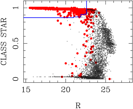
Figure 8: class_star values of the objects that are classified as point sources in the five and seven passband colour catalogues (filled red circles). This panel shows the $R$-band based on the five passband catalogue as an example, and the full figure is only available through the on-line edition. Black dots represent the class_star values of the objects that are classified as “stellar” and that are ranked 1 and $\leq 3$ in the full five and full seven passband catalogue respectively, when applying the $\chi^{2}$-technique. mag_star_lim and class_star limits are indicated.

Figure 9: Fraction of objects that are classified as “stellar” and that are ranked 1 and $\leq 3$ in the full five and full seven passband catalogue respectively, when applying the $\chi^{2}$-technique and that have a class_star less than 0.1. mag_star_lim limits are indicated. This panel shows the $R$-band based on the five passband catalogue as an example and the full figure is only available through the on-line edition.

7.6 Spectral types and data tables

Tables 3 and 4 give the first entries of the stellar catalogue in respectively five and seven bands. The tables give the following information: in column (1) the EIS identification number; in columns (2) and (3) the J2000 coordinates; in columns (4) - (13) for the five passband and columns (4) - (17) for the seven passband the magnitude (Vega system) and the SExtractor error (upper limits are indicated by a $-1$; in column (14) (respectively column (18) in the seven passband) the assigned spectral type, with the following meaning:

• Prefix “MS”. Templates for normal O to M stars from the Pickles (1998) library. Stars that are detected in fewer than three bands and therefore have not been fitted by the $\chi^{2}$-technique are listed as “dummy” here.

• Prefix “WD”. Templates for WDs from the models provided by D. Köster (the numbers indicate effective temperature and $\log g$), Ibata et al. (2000; the observed spectrum of F351-50, F821-07) or Oppenheimer et al. (2001; the observed spectrum of WD 0346+246).

• Prefix “LMS”. Templates for Low Mass Stars from Chabrier et al. (2000). The prefix is followed by a number indicating $T_{\rm eff}/100$ and the type of model used (NeGen = Next Generation, AMESd = DUSTY, or AMESc = CONDENSED, as defined in Chabrier et al. 2000).

Tables 5, 6, 7 and 8 give the first entries of the likely QSOs and unresolved galaxies in the five and seven passbands as identified by the procedure in Sect. 4. The information listed is the same as in the previous tables, except that in the last column the photometric redshift is listed for the QSOs, and the type of galaxy (following Coleman et al. 1980) and photometric redshift for the unresolved galaxies as determined by the spectral template fitting method.

The complete tables can be retrieved from the CDS or from the URL “http://www.eso.org/science/eis/eis_pub/eis_pub.html”.

Table 3: First 15 entries of the stellar catalogue in five passbands.

Table 4: First 15 entries of the stellar catalogue in seven passbands.

Table 5: First 15 entries of the likely QSOs in five passbands.

Table 6: First 15 entries of the likely QSOs in seven passbands.

Table 7: First 15 entries of the likely unresolved galaxies in five passbands.

Table 8: First 15 entries of the likely unresolved galaxies in seven passbands.

8 Summary and conclusions

This paper describes the procedures adopted in the construction of multi-colour stellar catalogues, suitable for statistical studies, extracted from multi-band imaging data. The procedure involves several steps among which: a magnitude-dependent scheme to morphologically classify sources identified using SExtractor; a procedure to combine the information available in catalogues extracted from images taken in different passbands; and the use of a $\chi^{2}$-technique to assign spectral types to the sources using the multi-band information. This allows to minimise the contamination of the stellar catalogue by QSOs and unresolved galaxies, and to assign spectral types for the stars, which are included in the stellar catalogues presented in this paper.

The methodology outlined here is applied to the first data set released for the DPS, the CDF-S. The 90% completeness limits are estimated to be approximately $U$ = 23.8, $B$ = 24.0, $V$ = 23.5, $R$ = 23.0, $I$ = 21.0, $J$ = 20.5, $K$ = 19.0. To assess the quality of the catalogues produced, number-counts, colour-colour and colour-magnitude diagrams, and colour-distributions derived from the data are compared to those obtained from simulated catalogues. Mock catalogues are created using a Galactic model based on population synthesis (described by parameters set by independent data), an error model describing the expected photometric errors, saturation and completeness as derived from the data. Even though no attempt is made to fine tune the Galactic model parameters the agreement between real and simulated data is remarkable, serving as a good indicator of the reliability of the catalogues produced. The comparison also suggests that the depth of the data is suitable to constrain the IMF and/or SFR of low-mass stars.

This paper represents a first attempt to define procedures to produce well-defined, deep stellar catalogues with minimal contamination by QSOs and unresolved galaxies. The results are encouraging and demonstrate the valuable contribution that the homogeneous multi-band optical/infrared data set from DPS, probing different directions of the Galaxy, will make when completed.

Appendix A Determining mag_star_lim and class_star_lim

Figure 10: class_star as a function of $R$-band magnitude, with the binning in magnitude and class_star indicated, for the first pass (top), and second pass (bottom, without data points for clarity). The hatched bin is the one that defines the background of galaxies.

This appendix gives a brief technical description of the way class_star_lim and mag_star_lim are determined in the present paper. Refinements of this scheme might be considered in the future after completion of the DPS survey (12 times the area under consideration here in different directions) and analysis of their respective stellar catalogues, spectroscopic follow-up studies that indicate the (in)correctness of the assigned spectral types, or more extensive numerical simulations including galaxies and QSOs.

One way to analyse a diagram like Fig. 1 is to set two levels of significance. The first, $t_{1}$, setting, for a fixed magnitude range, the level of significance of detecting stars against the background of galaxies at some value of class_star, and $t_{2}$, setting the level of significance of detecting stars at some magnitude, given a fixed range in class_star.

This idea is implemented in the following way. The first step is to allow for the single passband catalogue to be cut at a magnitude error level, and keeping only objects with “good” SExtractor flags.

For the present analysis, only objects with SExtractor flag $<$4 are kept and the default cut of S/N $>2$ is imposed. The objects retained are divided in bins of magnitude and class_star. Instead of using a fixed bin size in magnitude and class_star the bins are constructed in such a way that they contain an equal number of objects, that is, the width of the bin becomes the variable, rather than the number of objects in a bin of fixed size. The number of bins used is set automatically and is based on the total number of objects.

This is illustrated in Fig. 10 (top panel) for the $R$-band, where the objects are divided into 14 bins in magnitude and 53 bins in class_star in the first pass. When the density of objects is high the individual bins in class_star are no longer discernible.

For each magnitude bin, the distribution over class_star is analysed in the following way. The bin with the largest width in class_star is considered to define the background of galaxies (indicated by the hatched area in Fig. 10). A correction is made for the number of galaxies relative to the total number of objects in that bin based on the ratio of the number of objects below this bin to the total number of objects. For simplicity it is assumed that the background level is constant for the bins at higher class_star. The mean and rms (based on $\sqrt{N}$ statistics) per unit class_star are determined. This is a necessary step as all bins have a different width. For the bins that have a class_star value higher than that defining the background bin, the background level expected for that bin width is subtracted and divided by the rms level expected for that bin width. This gives a significance level per bin, ${\sigma}_{\rm bin}$. For an external threshold value, $t_{1}$, the lowest bin that has a significance above this threshold is determined and, by linear interpolation using the next highest bin, the final value for class_star_lim for that magnitude bin is calculated. In addition, all the bins that have a class_star larger than the bin that defines ${\sigma}_{\rm bin}$ are combined and a similar significance level for the group of stars as a whole (${\sigma}_{\rm group}$) is computed. Once the loop over the magnitude bins is completed, and given a second external threshold level, $t_{2}$, that magnitude bin is determined where $t_{2}>{\sigma}_{\rm group}$. By linear interpolation using the next brightest magnitude bin, the final value for mag_star_lim is computed. Additionally, the magnitude, $m_{\rm cut}$, is determined below which stars can not be recognised with any confidence. Then, for a bin in magnitude to the left of mag_star_lim (since mag_star_lim signifies a right-sided cut-off) and containing an equal number of objects as before, the binning in class_star and the analysis to derive the value for class_star_lim is repeated. This whole procedure is done twice, the first time using all objects that have passed the selection on magnitude error and SExtractor flag, and a second pass only retaining objects brighter than $m_{\rm cut}$. This allows for a better sampling over the magnitude interval where stars can be identified. The binning for the second pass and the effect of only retaining objects brighter than $m_{\rm cut}$ is illustrated in the bottom panel of Fig. 10. Figure 1 shows for the $R$-band the distribution over class_star and class_star_lim and mag_star_lim for the adopted choice of $t_{2}=30$ and $t_{1}=80$.

An independent check on the scheme presented, is to consider galaxy counts as the complement to the objects selected to be point sources, the argument being that if one is too liberal in the choice of mag_star_lim and class_star_lim to classify stars, the remaining number of “non-stars” could be inconsistent with known galaxy counts. In $B$, $R$ and $K$ the number of observed objects in the colour catalogue not classified as stars in the 0.5 mag bin below the faintest derived mag_star_lim limit (i.e. $23.35<B<23.85$, $22.25<R<22.75$, $18.30<K<22.80$) are, respectively, 2209, 1935 and 389. The number density of galaxies quoted in the literature is between 6500-11000, 5000-9000 and 4000-8000 per deg² per 0.5 magnitude bin in $BRK$ respectively (see the extensive compilation at http://star-www.dur.ac.uk/$\sim$nm/pubhtml/counts/counts.html for detailed references). The predicted number of galaxies for the effective area is 1710-2893, 1315-2367 and 371-742 in $BRK$ respectively, in agreement with the numbers observed, and indicating that the choice of mag_star_lim and class_star_lim to classify stars is not too liberal.