Analytic expressions for mean magnification by a quadrupole gravitational lens

Abstract

We derive an analytic expression for the mean magnification due to strong gravitational lensing, using a simple lens model, a singular isothermal sphere embedded in an external shear field. We compute separate expressions for 2-image and 4-image lensing. For 4-image lensing, the mean magnification takes a particularly simple form: $\left<\mu_{4}\right>=\frac{3.6}{\gamma\left(1-\gamma^{2}\right)}$, where $\gamma$ is the external shear. We compare our analytic results to a numerical evaluation of the full magnification distribution. The results can be used to understand the magnification bias that favors the discovery of four-image systems over two-image systems in flux-limited lens surveys.

1 Introduction

There have been several systematic surveys for examples of multiple-image gravitational lensing of extragalactic sources, both at optical wavelengths (e.g., Maoz et al., 1993; Surdej et al., 1993; Gregg et al., 2001) and radio wavelengths (Burke et al., 1993; King et al., 1999; Winn et al., 2000; Browne et al., 2002). The interpretation of the number of lensed sources that are detected in a flux-limited survey depends critically on the factors by which the sources are magnified. Lensed objects are drawn from a parent population with smaller fluxes than their unlensed counterparts. One therefore samples a fainter portion of the source luminosity function and a more distant range of source redshifts. This well-known “magnification bias” also affects the relative frequencies of different lens morphologies. Four-image lenses are more highly magnified than two-image lenses, and are subject to a stronger magnification bias.

Early studies of lens statistics used lens models with circular symmetry, such as singular isothermal spheres, for which the magnification bias is easy to calculate (e.g., Turner, Ostriker, & Gott, 1984). However, symmetric models only produce 2-image lenses and cannot be used to interpret the statistics of each morphology separately. More recently, numerical studies have been performed with more realistic elliptical lens models (e.g., King & Browne, 1996; Wallington & Narayan, 1993; Keeton, Kochanek, & Seljak, 1997; Rusin & Tegmark, 2001). While numerical calculations are certainly valuable, they tend to obscure the roles of competing contributions to what is being calculated. Analytic forms for such things as luminosity functions and magnifications may be no more accurate, but they produce results that are more readily understood.

With this motivation we examined a number of simple elliptical lens models and found one for which the mean magnification can be computed analytically, for both 2-image and 4-image lensing. The model is a singular isothermal sphere in an external shear field (SIS+XS), which is physically motivated and widely used.

In the next section we briefly review the mathematics and the qualitative features of lensing by non-circular potentials. In § 3, we specialize to the SIS+XS and derive the analytic expressions for all of the relevant quantities, including the mean magnification. Finally, in § 4 we compare our result to the full numerical evaluation of the magnification distribution, and remark on applications to the interpretation of lensing statistics.

2 Review of lensing by elliptical potentials

Lensing theory is well developed and has been expounded in detail by Schneider, Ehlers, & Falco (1992), among others. The particular problem of lensing by elongated potentials has been lucidly described by Blandford & Narayan (1986). Here we briefly review only those concepts that are required to follow the calculations presented in § 3.

We use the conventional definition of the lens potential,

$$\psi(r,\theta)\equiv\frac{2}{c^{2}}\frac{D_{ls}}{D_{l}D_{s}}\int_{0}^{\infty}\Phi(D_{l}{\mathbf{r}},z)dz,$$ (1)

in which $\Phi$ is the Newtonian gravitational potential of the galaxy; ${\mathbf{r}}$ is the sky-plane angular displacement; $z$ is the line-of-sight coordinate; and $D_{l}$, $D_{s}$, and $D_{ls}$ are the angular-diameter distances to the lens, to the source, and between lens and source, respectively. With this definition, the correspondence between source position ${\mathbf{s}}$ and image position ${\mathbf{r}}$ is

$${\mathbf{s}}={\mathbf{r}}-{\mathbf{\nabla}}_{{\mathbf{r}}}\psi({\mathbf{r}}).$$ (2)

The inverse magnification of a particular image $i$ is given by

$$\mu_{i}^{-1}=\left(1-\frac{\partial^{2}\psi}{\partial x^{2}}\right)\left(1-\frac{\partial^{2}\psi}{\partial y^{2}}\right)-\left(\frac{\partial^{2}\psi}{\partial x\partial y}\right)^{2},$$ (3)

which is negative when the image and source have opposite parity. For a survey in which sources are selected by total flux, the relevant quantity is the total magnification $\mu_{t}({\mathbf{s}})=\sum|\mu_{i}({\mathbf{s}})|$, the sum of the unsigned magnifications of all images of a source located at ${\mathbf{s}}$.

Most of the observed galaxy lenses can be described (at least qualitatively) using centrally concentrated, singular potentials. If the isopotential contours are only moderately elliptical, such potentials produce either 1, 2, or 4 images of a background source, in locations that can be understood with reference to the curves plotted in the top two panels of Figure 1. The curves are plotted for the SIS+XS, but the following discussion applies to many singular elliptical potentials.

Figure 1: Top. Source plane (left) and image plane (right) for the SIS+XS with $b=1$ and $\gamma=0.2$. The curves discussed in § 2 are labeled. The regions are labeled by image multiplicity, e.g., a point source in a region of the source plane marked “4” corresponds to four points in each of the four regions of the image plane marked “4.” Bottom. Same, but for $\gamma=0.45$.

For a source outside the radial caustic, one image is produced outside the 1–2 transition locus. A source on the radial caustic corresponds to one image on the 1–2 transition locus and another image at the origin, with zero flux. If the source moves from the radial caustic to the astroid caustic, the outer image moves to the outer 2–4 transition locus, while the inner image acquires a nonzero flux and moves to the inner 2–4 transition locus. On the astroid caustic, three images are produced: one on each of the 2–4 transition loci; and one on the critical curve, with infinite flux. Inside the astroid caustic, the latter image splits into two images with finite flux, and the result is one image in each of the regions marked “4” in Figure 1. The caustics and critical curve are well known to those who study gravitational lensing, but the transition loci receive less attention than they deserve—in particular, they are crucial for our calculation of mean magnification.

For more elongated potentials, two cusps of the astroid caustic pierce the radial caustic and are often referred to as “naked cusps.” The relevant curves in the source plane and the image plane are shown in the bottom panels of Figure 1. A source inside a naked cusp corresponds to three images located on the same side of the origin as the source—one in each of the three regions marked “3” in Figure 1.

If the source position is random, the cross section for producing 4 images, $\sigma_{4}$, is the total area within the 4-image region of the source plane (marked “4” in Figure 1). The 2-image cross-section is the area of the 2-image region, and the 3-image cross-section is the area of the 3-image region. The cross-section for multiple imaging is $\sigma_{m}=\sigma_{2}+\sigma_{3}+\sigma_{4}$.

The mean magnification for multiple-image lensing is the average value of the total magnification for all source positions that result in more than one image:

$$\left<\mu_{m}\right>=\frac{\int\mu_{t}({\mathbf{s}})d{\mathbf{s}}}{\int d{\mathbf{s}}}=\frac{\int_{\hbox{\footnotesize mult}}d{\mathbf{r}}}{\int d{\mathbf{s}}},$$ (4)

where the integral of $d{\mathbf{r}}$ extends over the region in the image plane in which multiple images are found. Eq. 4 holds because the Jacobian for the ${\mathbf{s}}\rightarrow{\mathbf{r}}$ transformation is equal to the magnification. Alternatively, one can visualize the calculation as follows. Because lensing conserves surface brightness, a source consisting of uniform brightness in the region formed by the union of the caustics will result in an image of uniform brightness within the union of the transition loci. The mean magnification for multiple-image lensing, which we denote $\left<\mu_{m}\right>$, is the ratio of the image area to the source area. The mean magnification of 4-image lenses, denoted $\left<\mu_{4}\right>$, is the ratio of 4-image region of image space and the 4-image region of source space. The mean magnification of 2-image and 3-image lenses can be visualized in a similar manner.

Of the approximately 100 observed cases of multiple-image gravitational lensing by galaxies, almost none require naked cusps for explanation. The one possible exception is APM 08279+5255 (Lewis et al., 2002). Because naked-cusp systems are apparently rare in nature, and because the calculations described below cannot be done analytically for naked-cusp systems, in this paper most of our attention will be on systems in which the astroid caustic is interior to the radial caustic.

In that case, to find the cross-sections and mean magnifications for 2-image and 4-image lensing, it is sufficient to calculate the areas enclosed by the radial caustic ($A_{r}$), astroid caustic ($A_{a}$), the 1–2 transition locus ($A_{t}$), and the inner and outer 2–4 transition loci ($A_{i}$ and $A_{o}$). As long as the astroid caustic is contained entirely within the radial caustic, we have:

$$\sigma_{4} = A_{d}$$

$$\sigma_{2} = A_{r}-A_{d}$$

$$\left<\mu_{4}\right> = \frac{A_{o}-A_{i}}{A_{d}}$$

$$\left<\mu_{2}\right> = \frac{A_{t}-A_{o}+A_{i}}{A_{r}-A_{d}}$$ (5)

3 Analytic expressions for the SIS+XS

We concentrate on the case of a singular isothermal sphere in an external shear field (SIS+XS), for which the potential is

$$\psi(r,\theta)=br+\frac{\gamma r^{2}}{2}\cos 2\theta.$$ (6)

Here $(r,\theta)$ are polar coordinates in the image plane, $b$ is the Einstein ring radius (which sets the mass scale of the lens), and $\gamma$ is the magnitude of the external shear. The SIS is an idealization of a spherical dark-matter halo with a flat rotation curve, and the external shear is a non-circular perturbation. This potential can be thought of as a truncated multipole expansion of the lens potential (see, e.g., Kovner, 1987; Schneider & Weiss, 1991; Trotter, Winn, & Hewitt, 2000). The SIS+XS has been used extensively in the literature to model observed lenses, often as a starting point for more complicated models (see, e.g., Kochanek, 1991; Keeton, Kochanek, & Seljak, 1997; Lehár, 1997; Schechter et al., 1997).

By computing the second derivatives of this potential and using Eq. 3, we obtain the magnification

$$\mu^{-1}=1-\gamma^{2}-\frac{b}{r}\left(1-\gamma\cos 2\theta\right).$$ (7)

We now derive expressions for all the relevant curves and the areas enclosed by them. We identify the radial caustic $(x_{r},y_{r})$ by requiring that it map to the origin under Eq. 2, obtaining

$$x_{r}=-b\cos\theta$$

$$y_{r}=-b\sin\theta,$$ (8)

which is a circle of radius $b$, enclosing an area $A_{r}=\pi b^{2}$.

Next, we identify the 1–2 transition locus by reverse-mapping the radial caustic back into the image plane, and finding the non-zero solution $r_{t}(\theta_{t})$:

$$x_{r}=-b\cos\theta=\left(1-\gamma\right)r_{t}\cos\theta_{t}-b\cos\theta_{t}$$

$$y_{r}=-b\sin\theta=\left(1+\gamma\right)r_{t}\sin\theta_{t}-b\sin\theta_{t}.$$ (9)

We eliminate the parameter $\theta$ by squaring and adding the equations, leading to the solution

$$r_{t}(\theta_{t})=2b\left(\frac{1-\gamma\cos 2\theta_{t}}{1-2\gamma\cos 2\theta_{t}+\gamma^{2}}\right).$$ (10)

The area enclosed by the 1–2 transition locus can be expressed in terms of definite integrals that are analytically tractable:

$$A_{t} = \frac{1}{2}\int_{0}^{2\pi}r_{t}^{2}d\theta_{t}$$

$$= 8b^{2}\int_{0}^{2\pi}\left[\frac{1}{1-2\gamma\cos 2\theta+\gamma^{2}}-\frac{\gamma^{2}(1-\cos 4\theta)}{(1-2\gamma\cos 2\theta+\gamma^{2})^{2}}\right]d\theta$$

$$= 4\pi b^{2}\left(\frac{1-\frac{\gamma^{2}}{2}}{1-\gamma^{2}}\right).$$

To identify the critical curve $r_{c}(\theta_{c})$, we require the inverse magnification $\mu^{-1}$ given by Eq. 7 to be zero, obtaining

$$r_{c}(\theta_{c})=\frac{b(1-\gamma\cos 2\theta_{c})}{1-\gamma^{2}}.$$ (12)

We obtain parametric equations for the astroid caustic $(x_{a},y_{a})$ by requiring the astroid caustic to map to the critical curve under the lens mapping, Eq. 2:

$$x_{a} = -\frac{2b\gamma}{1+\gamma}\cos^{3}\theta_{c}$$

$$y_{a} = \frac{2b\gamma}{1-\gamma}\sin^{3}\theta_{c}.$$ (13)

The maximum value of $x_{a}$ is $x_{*}=\frac{2b\gamma}{1+\gamma}$, and the area within the astroid caustic is

$$A_{a}=4\left|\int_{0}^{x_{*}}y_{a}dx_{a}\right|=\frac{16b^{2}\gamma^{2}}{1-\gamma^{2}}\int_{0}^{\frac{\pi}{2}}3\sin^{4}\theta\cos^{2}\theta d\theta=\frac{3\pi b^{2}}{2}\frac{\gamma^{2}}{1-\gamma^{2}}.$$ (14)

We note that the astroid caustic is completely interior to the radial caustic for $\gamma<\frac{1}{3}$.

Under the lens mapping, the astroid caustic has 2 images apart from the critical curve: the inner 2–4 transition locus, $r_{i}(\theta_{i})$, and the outer 2–4 transition locus, $r_{o}(\theta_{o})$. In order to solve for these transition loci, which we refer to generically as $r_{4}(\theta_{4})$, we insert the parametric equations 13 into Eq. 2:

$$-\frac{2b\gamma}{1+\gamma}\cos^{3}\theta_{c} = \left(1-\gamma\right)r_{4}\cos\theta_{4}-b\cos\theta_{4}$$

$$\frac{2b\gamma}{1-\gamma}\sin^{3}\theta_{c} = \left(1+\gamma\right)r_{4}\sin\theta_{4}-b\sin\theta_{4}.$$ (15)

After eliminating $r_{4}$ from this pair of equations, and defining $t\equiv\cos\theta_{c}$, we obtain

$$(\cos\theta_{4}-t)^{2}\left[\cos^{2}\theta_{4}+2t(1-t^{2})\cos\theta_{4}-t^{4}\right]=0,$$ (16)

which has three solutions: the double root $\cos\theta_{4}=t$ corresponding to the critical curve, and the 2–4 transition loci

$$\cos\theta_{i,o}=t\left(t^{2}-1\pm\sqrt{t^{4}-t^{2}+1}\right).$$ (17)

We insert these solutions for $\cos\theta_{4}$ into the first expression of Eqs. 15 to obtain parametric equations for the 2–4 transition loci:

$$r_{4}(t)=\frac{b}{1-\gamma}\left[1-\frac{2\gamma t^{3}}{(1+\gamma)\cos\theta_{4}(t)}\right].$$ (18)

It is possible to find the area within each locus separately—but for the calculation of mean magnification, the key quantity is the area between the 2–4 transition loci, which is (after lengthy algebra)

$$A_{o}-A_{i}=4\times\frac{1}{2}\int_{0}^{\frac{\pi}{2}}(r_{o}^{2}-r_{i}^{2})d\theta=\frac{4\pi b^{2}\gamma}{(1-\gamma^{2})^{2}}(I_{1}+I_{2}\gamma),$$ (19)

where $I_{1}$ and $I_{2}$ are defined as

$$I_{1} = \frac{2}{\pi}\int_{0}^{\frac{\pi}{2}}\frac{t_{i}^{3}(\theta)-t_{o}^{3}(\theta)}{\cos\theta}d\theta$$

$$I_{2} = \frac{2}{\pi}\int_{0}^{\frac{\pi}{2}}\left[\frac{t_{i}^{3}(\theta)-t_{o}^{3}(\theta)}{\cos\theta}+\frac{t_{i}^{6}(\theta)-t_{o}^{6}(\theta)}{\cos^{2}\theta}\right]d\theta,$$ (20)

and $t_{i,o}(\theta)$ are the inverse relations of Eq. 17. It is straightforward to prove $I_{2}=0$ by demonstrating that the integrand is antisymmetric about $\theta=\frac{\pi}{4}$ (see Finch, 2001), and $I_{1}$ is a dimensionless number independent of $b$ and $\gamma$. Numerically we find $I_{1}=1.35111$, leading to the result

$$A_{o}-A_{i}=\frac{4\pi b^{2}I_{1}\gamma}{(1-\gamma^{2})^{2}}\approx\frac{17b^{2}\gamma}{(1-\gamma^{2})^{2}}.$$ (21)

Now that all of the relevant curves and areas have been calculated, we compute cross sections and mean magnifications using Eqs. 5. We emphasize that these results are only valid for $\gamma<\frac{1}{3}$, when the astroid caustic is completely interior to the radial caustic. To find mean magnifications for $\gamma>\frac{1}{3}$, one must determine the intersection points of the various curves, for which we do not have analytic solutions. In § 4 we present numerical results for this case.

The SIS+XS is the only example we have found that has all the qualitative features desired of a model for an elliptical potential and for which the areas bounded by the transition loci are all analytic. An example of another commonly-used potential for which we do not have analytic formulas for all the areas is

$$\psi(r,\theta)=br+\gamma br\cos 2\theta,$$ (22)

which can be thought of as a lowest-order multipole expansion of the singular isothermal ellipsoid (SIE) density distribution (see, e.g., Kormann, Schneider, & Bartelmann, 1994). The astroid caustic is contained completely within the radial caustic for $\gamma<\frac{1}{5}$. For this potential we found analytic expressions for all the curves except the 1–2 transition locus, using a procedure similar to the one described above. We were therefore unable to compute $\left<\mu_{2}\right>$, but all the other quantities are listed in Table 1.

Table 1: Cross sections and mean magnifications

$\psi(r,\theta)$	$\gamma_{\hbox{max}}$	$\sigma_{2}$	$\sigma_{4}$	$\left<\mu_{2}\right>$	$\left<\mu_{4}\right>$
$br+\frac{\gamma r^{2}}{2}\cos 2\theta$	$\frac{1}{3}$	$\pi b^{2}\left(\frac{1-\frac{5}{2}\gamma^{2}}{1-\gamma^{2}}\right)$	$\frac{3\pi b^{2}}{2}\frac{\gamma^{2}}{1-\gamma^{2}}$	$4\times\frac{\left(1-\frac{\gamma^{2}}{2}\right)\left(1-\gamma^{2}\right)-I_{1}\gamma}{\left(1-\frac{5\gamma^{2}}{2}\right)\left(1-\gamma^{2}\right)}$	$\frac{8I_{1}}{3\gamma(1-\gamma^{2})}$
$br+\gamma br\cos 2\theta$	$\frac{1}{5}$	$\pi b^{2}\left(1-\frac{15}{2}\gamma^{2}\right)$	$6\pi b^{2}\gamma^{2}$	$\cdots$	$\frac{4I_{1}}{3\gamma}$

4 Discussion

To put the analytic results in context, we numerically computed the full magnification distribution for multiple imaging by the SIS+XS, denoted $P_{m}(\mu$). We parameterized the points within the radial caustic and computed the total magnification of each point, by inverting Eq. 2 to find the images and Eq. 7 to derive the magnifications. We performed this procedure separately for the 2-image and 4-image regions of the source plane, so that the magnification distribution for each morphology ($P_{2}$ and $P_{4}$) could be computed separately. The results are plotted in Fig. 2 for the case $\gamma=0.2$.

Figure 2: Probability distribution of magnification by the SIS+XS model, shown here for the case $\gamma=0.2$. The 2-image distribution ($P_{2}$) and the 4-image distribution ($P_{4}$) are plotted separately. The minimum magnifications, given by Eqs. 23 and 24, are marked.

The general features of the distribution can be readily understood. The minimum magnification occurs when the source is on the $x$-axis of the radial caustic, giving

$$\mu_{2,\hbox{\footnotesize min}}=\frac{2}{\left(1+3\gamma\right)\left(1-\gamma\right)}.$$ (23)

There is a discontinuity at the minimum magnification for 4-image systems, which occurs for a source at the origin:

$$\mu_{4,\hbox{\footnotesize min}}=\frac{2}{\gamma\left(1-\gamma^{2}\right)}.$$ (24)

The high magnification tail is produced by sources in the vicinity of the astroid caustic. It can be shown generically that the asymptotic probability for caustic-dominated events varies as $\mu^{-3}$ (see, e.g., Blandford & Narayan 1987; or Schneider, Ehlers, & Falco 1992, p. 319), and indeed the logarithmic slope of $P_{4}$ as computed numerically is $-3.1$. The downward kink between $\mu=\mu_{2,\hbox{\footnotesize min}}$ and $\mu_{4,\hbox{\footnotesize min}}$ occurs at the minimum magnification for a source just outside the astroid caustic.

The number of multiple-image lenses in a flux-limited sample can be determined from the magnification distribution. As described in detail by Turner, Ostriker, & Gott (1984), in a survey of objects with intrinsic luminosity function $\phi(L,z)$ and a flux limit corresponding to an intrinsic luminosity $L_{\hbox{\footnotesize lim}}$, the bias factor $B$ by which multiple-image lenses at a given redshift $z$ are over-represented is

$$B=\frac{\int_{L_{\hbox{\tiny min}}}^{\infty}dL\int_{\mu_{\hbox{\tiny min}}}^{\infty}\mu^{-1}P_{m}(\mu)\phi(\frac{L}{\mu},z)d\mu}{\int_{L_{\hbox{\tiny min}}}^{\infty}\phi(L,z)dL}.$$ (25)

The bias factors for 2-image and 4-image lensing can also be computed separately, by replacing $P_{m}$ with $P_{2}$ or $P_{4}$. For the common case that the luminosity function is approximated by a power law,

$$\phi(L,z)=\frac{\phi_{\star}(z)}{L_{\star}(z)}\times\left(\frac{L}{L_{\star}(z)}\right)^{-\beta},$$ (26)

the bias factor reduces to $B=\left<\mu^{\beta-1}\right>$, which is simply the mean magnification for $\beta=2$. As pointed out by Rusin & Tegmark (2001), the value $\beta=2$ happens to be a good approximation for the radio source populations that have been searched in recent lens surveys (JVAS, King et al. 1999; CLASS, Browne et al. 2002; Winn et al. 2000). Our analytic results are therefore directly relevant to this case, in which previous calculations were performed by numerical integration and Monte Carlo simulation.

For example, the JVAS and CLASS surveys have found roughly equal numbers of 2-image and 4-image lenses, a result that various authors have struggled to interpret because it seems to require a magnification bias for 4-image lensing that is larger than expected (King & Browne, 1996; Keeton, Kochanek, & Seljak, 1997; Rusin & Tegmark, 2001). A resolution considered by these authors is that the matter distribution in the lens galaxies is systematically more elongated than the observed light distribution of elliptical galaxies.

We can estimate of the required value of $\gamma$ from our calculations of mean magnification. The ratio of 4-image lenses to 2-image lenses, including the effect of magnification bias, is

$$\frac{N_{4}}{N_{2}}=\frac{\sigma_{4}}{\sigma_{2}}\times\frac{B_{4}}{B_{2}}.$$ (27)

For the SIS+XS model and a $\beta=2$ luminosity function, the result is

$$\frac{N_{4}}{N_{2}}=\frac{\sigma_{4}\left<\mu_{4}\right>}{\sigma_{2}\left<\mu_{2}\right>}=\frac{I_{1}\gamma}{\left(1-\frac{\gamma^{2}}{2}\right)\left(1-\gamma^{2}\right)-I_{1}\gamma}.$$ (28)

This result is rather specialized, depending as it does on the assumption of a particular lens model and source luminosity function, but it has the virtue of being analytic. To obtain equal numbers of 4-image and 2-image systems we require $\gamma=0.32$, for which $\sigma_{2}/\sigma_{4}$ and $B_{4}/B_{2}$ are both approximately 5.

For $\gamma>\frac{1}{3}$ one must also consider the possibility of 3-image systems produced by naked cusps. In this case the computation of areas in the image plane must be done numerically. Figure 3 shows the results of a numerical calculation of the relative areas of the 2-image, 3-image, and 4-image regions of the image plane, for $0<\gamma<1$. As before, if $\beta=2$ then this plot can also be interpreted as the expected fractions of 2-image, 3-image, and 4-image lenses discovered in a flux-limited survey. For $\gamma<\frac{1}{3}$ the results are identical to our analytic formula. For $\gamma=\frac{1}{3}$, naked-cusp images are possible but occur with vanishing probability; they constitute 10% of the lenses at $\gamma\approx 0.45$ and they dominate the sample for $\gamma>0.61$.

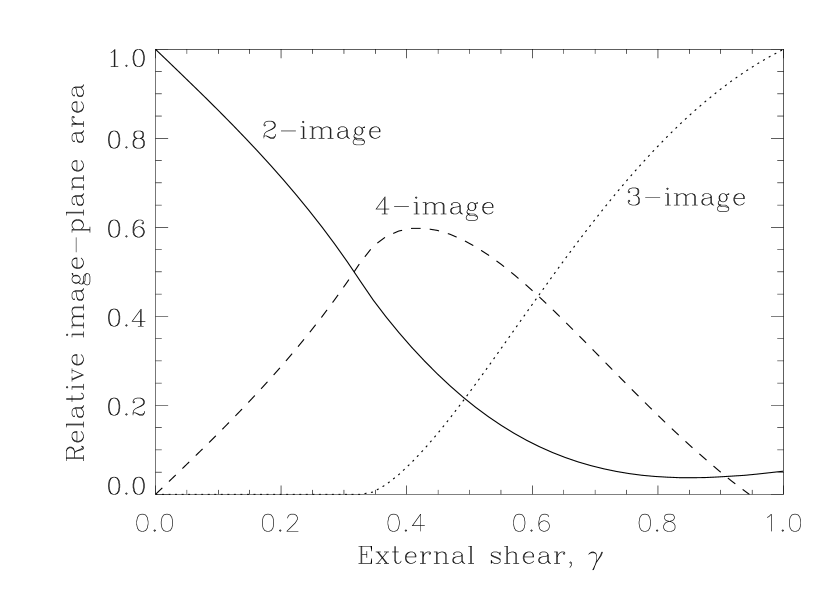
Figure 3: Numerical evaluation of the relative areas of the 2-image, 3-image, and 4-image regions of the image plane, for the SIS+XS model. Under the assumptions described in § 4 these curves also give the ratios of 2-image, 3-image, and 4-image systems expected in a flux-limited survey.

In more generic settings, the full magnification distribution is required. The 4-image magnification distribution, at least, can be approximated by $P_{4}(\mu)\propto\mu^{-3}$ for $\mu>\mu_{4,\hbox{\footnotesize min}}$. The mean of this approximate distribution is

$$\left<\mu_{4}\right>\approx\frac{\int_{\mu_{4,\hbox{\footnotesize min}}}^{\infty}\mu^{-2}d\mu}{\int_{\mu_{4,\hbox{\footnotesize min}}}^{\infty}\mu^{-3}d\mu}=\frac{4}{\gamma(1-\gamma^{2})},$$ (29)

which has the same dependence on $\gamma$ as the exact expression (see Table 1) and differs only by a constant fraction of $4/3.6$ or 11%.

5 Conclusion

We have described a geometrical method for computing the mean magnification for multiple imaging by non-circular lens potentials. For the special case of a singular isothermal sphere embedded in an external shear field, we have derived analytic expressions for the mean magnification for 2-image lensing and 4-image lensing. The results can be used, in certain circumstances, to compute the magnification bias for 2-image and 4-image lensing.

References

- Blandford & Narayan (1986) Blandford, R. & Narayan, R. 1986, ApJ, 310, 568
- Browne et al. (2002) Browne, I., et al. 2002, in preparation
- Burke et al. (1993) Burke, B., et al. 1993, in Sub-Arcsecond Radio Astronomy, eds. Davis, R.J. & Booth, R.S. (Cambridge: CUP), p. 123
- Evans & Wilkinson (1998) Evans, N.W. & Wilkinson, M.I. 1998, MNRAS, 296, 800
- Finch (2001) Finch, T., M.S. thesis, Massachusetts Institute of Technology
- Gregg et al. (2001) Gregg, M., et al. 2001, in Gravitational Lensing: Recent Progress and Future Goals, ASP Conference Proceedings, Vol. 237, eds. Brainerd, T. & Kochanek, C.S. (San Francisco: ASP), p. 41
- Jørgensen & Franx (1994) Jørgensen, I. & Franx, M. 1994, ApJ, 433, 553
- Keeton, Kochanek, & Seljak (1997) Keeton, C.R., Kochanek, C.S., & Seljak, U. 1997, ApJ, 482, 604
- King & Browne (1996) King, L. & Browne, I.W.A. 1996, MNRAS, 282, 67
- King et al. (1999) King, L., et al. 1999, MNRAS, 307, 225
- Kochanek (1991) Kochanek, C.S. 1991, ApJ, 373, 354
- Kormann, Schneider, & Bartelmann (1994) Kormann, R., Schneider, P., & Bartelmann, M. 1994, A&A, 284, 285
- Kovner (1987) Kovner, I. 1987, ApJ, 312, 22
- Lehár (1997) Lehár, J., et al. 1997, AJ, 114, 48
- Lewis et al. (2002) Lewis, G., et al. 2002, MNRAS, 330, L15
- Maoz et al. (1993) Maoz, et al. 1993, ApJ, 409, 28
- Rusin & Tegmark (2001) Rusin, D. & Tegmark, M. 2001, ApJ, 553, 709
- Schechter et al. (1997) Schechter, P.L., et al. 1997, ApJ, 475, L85
- Schneider, Ehlers, & Falco (1992) Schneider, P., Ehlers, J., & Falco, E. 1992, Gravitational Lenses (New York: Springer-Verlag)
- Schneider & Weiss (1991) Schneider, P. & Weiss, A. 1991, A&A, 247, 269
- Surdej et al. (1993) Surdej, J., et al. 1993, AJ, 105, 2064
- Trotter, Winn, & Hewitt (2000) Trotter, C., Winn, J.N., & Hewitt, J.N. 2000, ApJ, 535, 671
- Turner, Ostriker, & Gott (1984) Turner, E., Ostriker, J., & Gott, J.R. III 1984, ApJ, 284, 1
- Wallington & Narayan (1993) Wallington, S. & Narayan, R. 1993, ApJ, 403, 517
- Winn et al. (2000) Winn, J.N., et al. 2000, AJ, 120, 2868