Analytical Approach to the Mass Distribution Function of Subhalos and Cold Fronts in Galaxy Clusters

Abstract

We construct an analytical model of the mass distribution function of subhalos in a galaxy cluster in the context of the cold dark matter (CDM) theory. Our model takes account of two important effects; the high density of the precluster region and the spatial correlation of initial density fluctuations. For subhalos with small masses, the mass distribution function that our model predicts is intermediate between the Press-Schechter (PS) mass distribution function and a conditional mass distribution function as an extension of the PS formalism. We compare the results of our model with those of numerical simulations. We find that our model predictions are consistent with the mass and velocity distribution functions of subhalos in a cluster obtained by numerical simulations. We estimate the probability of finding large X-ray subhalos that often have “cold fronts”. The observed large X-ray subhalos and cold fronts may not always be the result of cluster mergers, but instead may be internal structures in clusters.

1 Introduction

It is generally believed that dark matter constitutes a large fraction of the mass in the universe. Among various theories of dark matter, cold dark matter (CDM) theory provides a remarkably successful description of large-scale structure formation, and it is in good agreement with a large variety of observational data. This model predicts that small objects are the first to form and these then amalgamate into progressively larger system. This means that galaxy clusters have formed via merging and accretion of galaxies or galaxy groups.

If the dark matter is actually the main component of galaxies and clusters, $N$-body simulations can be used to predict their bulk properties, such as position, mass, and size. However, it has proven difficult to find surviving substructure (subhalos) in virialized objects in $N$-body simulations. This apparent absence of substructure, known as “the overmerging problem,” reflects the fact that simulated subhalos are disrupted much more efficiently than real subhalos (Moore, Katz, & Lake, 1996).

Analytical studies showed that the overmerging problem was caused by poor force and mass resolutions (Moore et al., 1996). Klypin et al. (1999) estimated that the force and mass resolutions required for a simulated halo to survive in galaxy groups and clusters are extremely high: $\sim 1-3$ kpc and $10^{8}-10^{9}\;M_{\sun}$. Recently, simulations with roughly the required resolution have been done (Ghigna et al., 1998; Tormen, Diaferio, & Syer, 1998; Klypin et al., 1999; Okamoto & Habe, 1999; Colín et al., 1999; Moore et al., 1999; Jing & Suto, 2000; Ghigna et al., 2000; Gottlöber, Klypin, & Kravtsov, 2001; White, Hernquist, & Springel, 2001; Fukushige & Makino, 2001; Bullock et al., 2001). These simulations certainly showed that subhalos survive in clusters. Okamoto & Habe (1999) compared the mass distribution function (MDF) of subhalos with the Press-Schechter (PS) MDF (Press & Schechter, 1974) and a conditional MDF derived through an extension of the PS formalism (EPS; Bower, 1991; Bond et al., 1991; Lacey & Cole, 1993, see §3 for detail). They found that the MDF of subhalos in their simulated cluster at $z=0$ is similar to the PS MDF at $z=2$. It is also similar to the EPS MDF but the fit is a little worse. They suggested that the MDF of subhalos freezes out after the cluster had grown sufficiently, which in their simulation occurred at $z\sim 2$. Thus, the MDF of subhalos preserves the information about the growth of density fluctuations at that time. In other words, we can use observations of the MDF of subhalos at present to determine the hierarchical clustering which occurred in the past. However, the good match between the simulations and the PS MDF found by Okamoto & Habe (1999) is somewhat surprising as the PS MDF does not take into account the fact that the cluster subhalos are in a high density region. The EPS MDF does include the density effect, yet provides a slightly worse fit to the simulations than the PS MDF.

Another important factor that should be taken into account when the MDF of subhalos in a cluster is considered is the spatial correlation of initial density fluctuations. It has been shown that this spatial correlation does affect the MDF of dark halos in the whole universe (Yano, Nagashima, & Gouda, 1996; Nagashima, 2001). This means that one cannot ignore the effect of spatial correlation on the MDF of subhalos because these subhalos originated from density fluctuations that were close to one another. In this paper, we construct a model of the subhalo MDF in a cluster considering the effect of spatial correlations as well as the fact that cluster subhalos are located in a high density region. Of course, there are other mechanisms that could affect the MDF of subhalos especially after the cluster formation (e.g. tidal stripping). Although they should be taken into account in order to derive the MDF exactly, we do not consider them in our model for the sake of simplicity. Even so, our model should be useful to predict the MDF in the case where the mechanisms that occur after cluster formation are not very effective, and gives an upper limit to substructure if disruptive processes are important for a wide range of masses. Our analytic model is not affected by spatial and mass resolutions, which affect numerical simulations. It will be useful to compare with the results of numerical simulations to determine the effects of finite resolution. Even though some of the recent high-resolution simulations meet fully the conditions required to study subhalos (Klypin et al., 1999), comparing them with our model is still important. Such comparisons can serve as a check for the subhalo identification algorithm applied to the simulation results.

Both the MDFs predicted by our model and the results from numerical simulations should be compared with the observations. In the past, galaxies were used to derive the observed MDF in a cluster. In fact, Moore et al. (1999) compared their simulation results with the observational data from the Virgo cluster, although they used the circular velocity distribution function (VDF) of galaxies instead of the MDF. They showed that the simulation and observed VDFs are roughly consistent with one another. However, individual galaxies could not be used to detect massive subhalos, because the observed circular velocity (or velocity dispersion) of a galaxy is at most $v_{c}\sim 300\;\rm km\;s^{-1}$. On the other hand, numerical simulations suggest that clusters have subhalos with $v_{c}\gtrsim 300\;\rm km\;s^{-1}$ (Moore et al., 1999). Until recently, it was not understood whether the lack of galaxies with $v_{c}\gtrsim 300\;\rm km\;s^{-1}$ requires a lack of massive subhalos in a cluster, or whether this implies that galaxies have lower values of $v_{c}$ than would characterize the massive dark matter halos surrounding the galaxies. Recently, X-ray observations with the Chandra Observatory have found that some clusters have massive subhalos moving within the clusters which have not been disrupted (Markevitch et al., 2000; Vikhlinin, Markevitch, & Murray, 2001; Mazzotta et al., 2001, 2002; Sun et al., 2002). The contact surface between the cooler subhalo gas and the surrounding hot intracluster medium is called a “cold front”. The X-ray temperatures of these subhalos are $\sim 4-7$ keV, which is substantially higher that the kinetic temperatures one would derive from the motions of stars in the optical galaxies in the subhalos. The observations of these massive subhalos gives us important information about the massive end of the MDF.

The plan of our paper is as follows. In §2, we derive the MDF in clusters analytically. We discuss the resulting MDFs and compare them with those from numerical simulations in §3, We discuss the effect of tidal stripping and dynamical friction on the MDFs in §4. In §5, we derive the VDF of subhalos and compare these results with those of numerical simulations and observations of galaxies. We estimate the probability of finding massive X-ray subhalos and associated cold fronts in clusters in §6. Finally, §7 summarizes our conclusions.

2 Models

In this section, we derive the MDF of subhalos in a cluster including the effects of spatial correlations using the model of Yano et al. (1996). We use the so-called sharp $k$-space filter for density fluctuations following Yano et al. (1996). We assume that the primordial density field is a Gaussian random field.

First, we estimate the conditional probability, $P(r,M_{1},M_{2})$, of finding a region of mass $M_{1}$ with $\delta_{1}\geq\delta_{c1}$ at a distance $r$ from the center of an isolated, finite-sized object of mass $M_{2}$, provided that the object of mass $M_{1}$ is included in the object of mass $M_{2}$ $(>M_{1})$ with $\delta_{2}=\delta_{c2}$ at $r=0$. Here, we define $\delta_{M}$ as the smoothed linear density fluctuation of mass scale $M$, and $\delta_{1}=\delta_{M_{1}}$ and $\delta_{2}=\delta_{M_{2}}$. Moreover, we define $\delta_{c}(z)$ as the critical density threshold for a spherical perturbation to collapse by the redshift $z$, and $\delta_{c1}=\delta_{c}(z_{1})$ and $\delta_{c2}=\delta_{c}(z_{2})$. In the Einstein-de Sitter universe, $\delta_{c}(z)=1.69(1+z)$. While Yano et al. (1996) considered only the case of $\delta_{c1}=\delta_{c2}$, we consider the case of $\delta_{c1}\geq\delta_{c2}$ ($z_{1}>z_{2}$) in general. Because the covariance matrix for the Gaussian distribution for two variables $[\delta_{1}(r),\delta_{2}]$ is given by

$$\mbox{\boldmath$M$}=\left[\begin{array}[]{cc}\sigma_{1}^{2}&\sigma_{c}^{2}(r)\\ \sigma_{c}^{2}(r)&\sigma_{2}^{2}\\ \end{array}\right]\;,$$ (1)

the probability can be written as

$$P(r,M_{1},M_{2}) = p[\delta_{1}\geq\delta_{c1}|\delta_{2}=\delta_{c2}]$$ (2)

$$= p[\delta_{1}\geq\delta_{c1},\delta_{2}=\delta_{c2}]/p(\delta_{2}=\delta_{c2})$$

$$= \frac{1}{\sqrt{2\pi[1-\epsilon^{2}(r)]}}\int^{\infty}_{\nu_{1c}}\exp{\left\{\frac{-[\nu_{1}-\epsilon(r)\nu_{2c}]^{2}}{2[1-\epsilon^{2}(r)]}\right\}}d\nu_{1}\;,$$

where $\nu_{1}$ and $\nu_{2}$ are defined by

$$\nu_{1}\equiv\frac{\delta_{1}}{\sigma_{1}}\,,\,\nu_{2}\equiv\frac{\delta_{2}}{\sigma_{2}}\,,\,\sigma_{1}\equiv\sigma(M_{1})\,,\,\sigma_{2}\equiv\sigma(M_{2})\,,\,\nu_{1c}\equiv\frac{\delta_{c1}}{\sigma_{1}}\,,\,\nu_{2c}\equiv\frac{\delta_{c2}}{\sigma_{2}}\,,\,$$ (3)

respectively (Yano et al., 1996). In equations (3), $\sigma(M)$ is the rms density fluctuation smoothed over a region of mass $M$, and is given by

$$\sigma^{2}(M)=\frac{V}{(2\pi)^{3}}\int_{0}^{k_{c}(M)}|\delta_{k}|^{2}4\pi k^{2}dk\;.$$ (4)

In this equation, $V$ is the volume, $k$ is the wave number, and $\delta_{k}$ is the Fourier components of density fluctuations. The critical wave number, $k_{c}(M)$ is the wave number corresponding to mass scale $M$ and is given by $k_{c}(M)=\pi/(3M/4\pi\bar{\rho})$, where $\bar{\rho}$ is the current mean mass density of the universe. Moreover, $\epsilon(r)$ is defined by

$$\epsilon(r)\equiv\frac{\sigma_{c}^{2}(r)}{\sigma_{1}\sigma_{2}}\;,$$ (5)

$$\sigma_{c}^{2}(r)=\langle\delta_{2}(\mbox{\boldmath$r$}_{0})\delta_{1}(\mbox{\boldmath$r$}_{0}+\mbox{\boldmath$r$})\rangle=\frac{V}{(2\pi)^{3}}\int_{0}^{k_{c}(M_{2})}|\delta_{k}|^{2}\frac{\sin(kr)}{kr}4\pi k^{2}dk\;,$$ (6)

which corresponds to the two-point correlation function.

We can rewrite equation (2) as

$$P(r,M_{1},M_{2})=\frac{1}{\sqrt{2\pi}}\int_{\beta}^{\infty}e^{-y^{2}/2}dy\;,$$ (7)

where

$$\beta(r)=\frac{\nu_{1c}-\epsilon(r)\nu_{2c}}{\sqrt{1-\epsilon^{2}(r)}}=\frac{1}{\sqrt{1-\epsilon^{2}(0)\alpha^{2}(r)}}\frac{\delta_{c1}}{\sigma_{1}}\left[1-\frac{\delta_{c2}}{\delta_{c1}}\alpha(r)\right]\>,$$ (8)

and $\alpha(r)=\epsilon(r)/\epsilon(0)$. The spatially averaged conditional probability for $r<R$ is defined as

$$P(M_{1},M_{2})=\int_{0}^{R}P(r,M_{1},M_{2})4\pi r^{2}dr/\int_{0}^{R}4\pi r^{2}dr\>.$$ (9)

The definition of $P(M_{1},M_{2})$ (equations [7] and [9]) is similar to the probability that the density contrast on a scale of $M$ exceeds $\delta_{c}$ in field:

$$f(\geq\delta_{c},M)=\frac{1}{\sqrt{2\pi}}\int_{\delta_{c}/\sigma(M)}^{\infty}e^{-y^{2}/2}dy\;.$$ (10)

From this, the PS MDF can be obtained as

$$\tilde{n}_{\rm PS}dM=2\frac{\bar{\rho}}{M}\left|\frac{df}{dM}\right|dM\>,$$ (11)

(Press & Schechter, 1974).

Using the similarity between $f(\geq\delta_{c},M)$ and $P(r,M_{1},M_{2})$, we define the MDF of the collapsed objects (subhalos) in the region of a mass scale of $M_{0}$ by differentiating $P(M,M_{0})$ and multiplying it by 2 (PS approximation):

$$n_{\rm SPS}dM=2\frac{M_{0}}{M}\left|\frac{\partial P(M,M_{0})}{\partial M}\right|dM\>.$$ (12)

This expression is based on the usual PS assumptions. However, we emphasize that the MDF (equation [12]) includes the effect of the spatial correlation of fluctuations through the two-point correlation function (equation [6]). Moreover, it is the MDF in a high density region, rather than the MDF for an average region of the universe. As will shown in the next section, our model is a further extension of the EPS MDF by taking account of spatial correlations of halos. Thus, we refer to this MDF as SPS MDF. We assume that the region of the mass scale of $M_{0}$ will collapse into a cluster and the subhalos in the region also fall into the cluster. The density fluctuations in the cluster region should stop growing as the cluster grows, because the kinetic energy released at the cluster collapse allows the subhalos to move in the cluster, which prevents their further growth. We call the redshift when this occurs the effective formation redshift of the cluster, $z_{f}$. Thus, we use $\delta_{c1}=\delta_{c}(z_{f})$ or $z_{1}=z_{f}$ in equations (2) and (12).

Strictly speaking, the conditional probability $P(M_{1},M_{2})$ derived in this section is not sufficient to obtain the exact MDF. This is because an isolated object of mass scale $M_{2}$ must have the maximum peak density with $\delta_{2}=\delta_{c2}$ at $r=0$. Thus, we need an additional condition. However, Yano et al. (1996) showed that the effect is negligible as long as we consider a fluctuation power spectrum with an index of $n\lesssim-2$ and the mass scale with $\sigma(M)\gtrsim 1$. Our calculations in the following sections satisfy these conditions.

3 Mass Distribution Function

We calculate the MDF of subhalos in a cluster, $n_{\rm SPS}$, for a CDM universe with cosmological parameters of $\Omega_{0}=1$, $\lambda=0$, $\sigma_{8}=0.7$, $\Gamma=0.5$, and $h=0.5$, where $\sigma_{8}$ is the rms mass fluctuation on $8h^{-1}$ Mpc, and $\Gamma$ is the so-called shape parameter of the CDM spectrum. We use a Hubble constant of $H_{0}=100h\;\rm km\;s^{-1}\;Mpc^{-1}$. The cluster mass at $z_{0}=0$ is $M_{0}=4.3\times 10^{14}\;M_{\sun}$. These parameters are the same as those used for an ultra-high resolution numerical simulation done by Ghigna et al. (2000). We calculate the conditional probability, $P(M,M_{0})$, spatially averaged in a precluster region, $r<R=R_{0}$, where $R_{0}=(3M_{0}/4\pi\bar{\rho})^{1/3}$. From now on, we assume $R=R_{0}$ unless otherwise stated.

For comparison, we also calculated a conditional MDF, that is, the number of halos with mass between $M$ and $M+dM$ at $z_{f}$ that are in a halo of mass $M_{0}$ at $z_{0}$ ($M<M_{0}$, $z_{0}<z_{f}$). It is given by

$$n_{\rm EPS}(M,z_{f}|M_{0},z_{0})dM=\frac{M_{0}}{M}f(S,\omega|S_{0},\omega_{0})\left|\frac{dS}{dM}\right|dM\>,$$ (13)

where

$$f(S,\omega|S_{0},\omega_{0})dS=\frac{\omega-\omega_{0}}{(2\pi)^{1/2}(S-S_{0})^{3/2}}\exp\left[-\frac{(\omega-\omega_{0})^{2}}{2(S-S_{0})}\right]dS\;,$$ (14)

$S=\sigma^{2}(M)$, $S_{0}=\sigma^{2}(M_{0})$, $\omega=\delta_{c}(z_{f})$, and $\omega_{0}=\delta(z_{0})$ (Bower, 1991; Bond et al., 1991; Lacey & Cole, 1993). This formalism is often called the extended Press-Schechter formalism (EPS).

We note that the difference between $n_{\rm SPS}$ and $n_{\rm EPS}$ comes from whether the effect of the spatial correlation of fluctuations is included or not. If we ignore the spatial correlation, $P(M_{1},M_{2})$ should be written as

$$P(M_{1},M_{2}) = p(\delta_{1}\geq\delta_{c1}|\delta_{2}=\delta_{c2})$$ (15)

$$= \int_{\delta_{c1}}^{\infty}\frac{1}{\sqrt{2\pi(\sigma_{1}^{2}-\sigma_{2}^{2})}}\exp\left[-\frac{(\delta_{1}-\delta_{2c})^{2}}{2(\sigma_{1}^{2}-\sigma_{2}^{2})}\right]d\delta_{1}$$

$$= \frac{1}{\sqrt{2\pi}}\int_{\beta^{\prime}}^{\infty}e^{-y^{2}/2}dy\;,\;$$

where

$$\beta^{\prime}=\frac{1}{\sqrt{1-\epsilon^{2}(0)}}\frac{\delta_{c1}}{\sigma_{1}}\left(1-\frac{\delta_{c2}}{\delta_{c1}}\right)\>,$$ (16)

(see Yano et al., 1996). In this case, it can easily be shown that the right hand of equation (12) is identical to that of equation (13) (see Bower, 1991). We also note that at $r=0$, the right hand of equation (2) is identical to that of equation (15) (Yano et al., 1996). We refer the right hand of equation (15) as $P_{\rm EPS}(M_{1},M_{2})$, so that

$$n_{\rm EPS}\>dM=2\frac{M_{0}}{M}\left|\frac{\partial P_{\rm EPS}(M,M_{0})}{\partial M}\right|dM\>.$$ (17)

We would like to point out that the equation (9) gives the probability distribution of the mass of halo progenitors as $P_{\rm EPS}(M_{1},M_{2})$. Thus, it could be possible to construct dark halo merger trees including the spatial correlation of dark halos, which would be important for semi-analytic models of galaxy formation.

We also compare $n_{\rm SPS}$ with the conventional PS MDF (equation [11]). Instead of $\tilde{n}_{\rm PS}$, we use the MDF,

$$n_{\rm PS}dM=\frac{M_{0}}{\bar{\rho}}\tilde{n}_{\rm PS}dM=2\frac{M_{0}}{M}\left|\frac{df}{dM}\right|dM\>.$$ (18)

Of course, the PS MDF includes neither the effect of the spatial correlation of fluctuations nor that of the density excess in a precluster region.

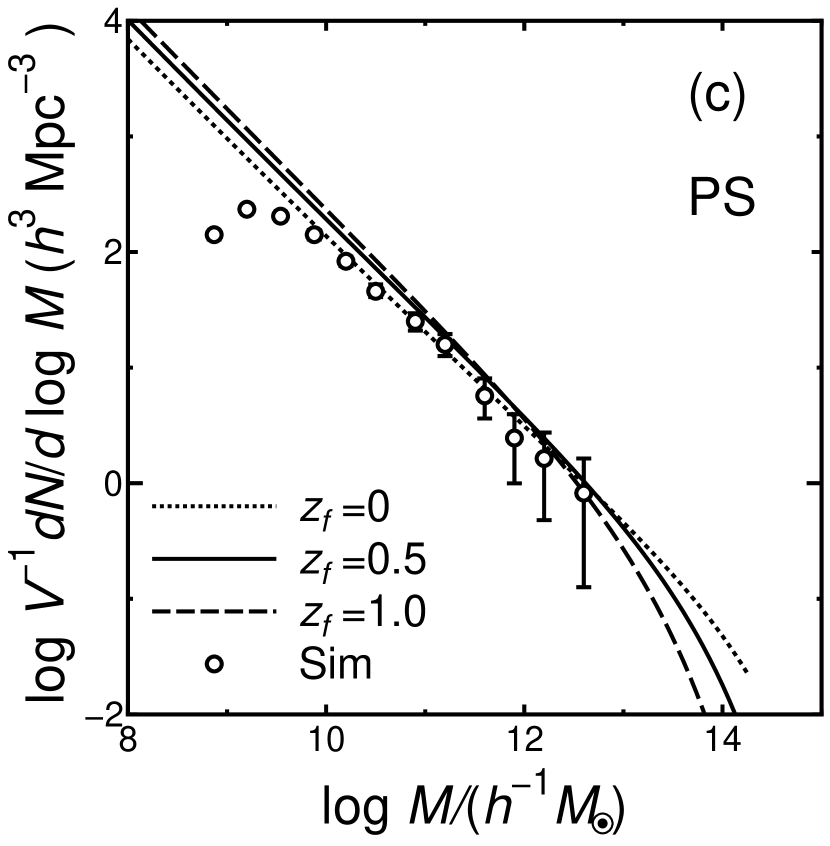
Figure 1: Subhalo mass distribution functions for $z_{f}=0$ or 0.1 (dotted lines), $z_{f}=0.5$ (solid lines), and $z_{f}=1.0$ (dashed lines). (a) $n_{\rm SPS}$, (b) $n_{\rm EPS}$, and (c) $n_{\rm PS}$. The MDF at $z=0$ obtained from the numerical simulation by Ghigna et al. (2000) is shown by the circles.

Figure 1 shows the three MDFs at $z=z_{0}=0$. For the vertical axes, we use

$$\frac{1}{V}\frac{dN}{dM}=\frac{n_{i}}{V}\>,$$ (19)

where $V=4\pi R_{c}^{3}/3$ and $i=$ SPS, EPS, and PS following Ghigna et al. (2000). We use capital $N$ for cumulative numbers from now on. The cluster radius, $R_{c}$, is the same for all the three models and is given by $R_{c}=(3M_{0}/4\pi\rho_{0})^{1/3}$, where $\rho_{0}$ is the average density of the cluster and is 178 times the critical density of the universe for our cosmological parameters. In equation (10), we use $\delta_{c}=\delta_{c}(z_{f})$.

As the effective formation redshifts of a cluster, we use $z_{f}=0$, 0.5, and 1 for $n_{\rm SPS}$ and $n_{\rm PS}$. On the other hand, if we chose $z_{f}=0$ in the EPS MDF, we would find trivially that $n_{\rm EPS}=0$ except at $M=M_{0}$. (That is, there are no subhalos except for the cluster itself.) Thus, for the EPS MDF we show the results for $z_{f}=0.1$, 0.5, and 1. The mass distribution function $n_{\rm SPS}$ increases with $z_{f}$ for smaller $M$, which is also true of $n_{\rm EPS}$ and $n_{\rm PS}$. Figure 1 also shows that $n_{\rm EPS}<n_{\rm SPS}<n_{\rm PS}$ for $z_{f}\sim 0=z_{0}$ and $M\lesssim 10^{12}\;M_{\rm\sun}$. This can be understood as follows: When $z_{f}\ll 1$ (or $\delta_{c}[z_{f}]\approx\delta_{c}[z_{0}]$), $M\ll M_{0}$ (or $\epsilon[0]\ll 1$), and $\delta_{c}(z_{f})/\sigma(M)\ll 1$, we obtain

$$\beta(r)\approx\frac{\delta_{c}(z_{f})}{\sigma(M)}\left[1-\frac{\delta_{c}(0)}{\delta_{c}(z_{f})}\alpha(r)\right]\>,$$ (20)

and

$$\beta^{\prime}\approx\frac{\delta_{c}(z_{f})}{\sigma(M)}\left[1-\frac{\delta_{c}(0)}{\delta_{c}(z_{f})}\right]\>.$$ (21)

This implies that

$$\beta^{\prime}<\beta<\delta_{c}(z_{f})/\sigma(M)\ll 1\>,$$ (22)

from equations (8) and (16) because $0\leq\alpha(r)\leq 1$. Thus, we obtain

$$\left|\frac{\partial P(r,M,M_{0})}{\partial M}\right|\approx\frac{1}{\sqrt{2\pi}}\left[1-\frac{\delta_{c}(0)}{\delta_{c}(z_{f})}\alpha(r)\right]\left|\frac{\partial}{\partial M}\frac{\delta_{c}(z_{f})}{\sigma(M)}\right|\>,$$ (23)

$$\left|\frac{\partial P_{\rm EPS}(M,M_{0})}{\partial M}\right|\approx\frac{1}{\sqrt{2\pi}}\left[1-\frac{\delta_{c}(0)}{\delta_{c}(z_{f})}\right]\left|\frac{\partial}{\partial M}\frac{\delta_{c}(z_{f})}{\sigma(M)}\right|\>,$$ (24)

$$\left|\frac{\partial f[\geq\delta_{c}(z_{f}),M]}{\partial M}\right|\approx\frac{1}{\sqrt{2\pi}}\left|\frac{\partial}{\partial M}\frac{\delta_{c}(z_{f})}{\sigma(M)}\right|\>.$$ (25)

from equations (7), (15), and (10). Since the relation

$$\left|\frac{\partial P_{\rm EPS}(M,M_{0})}{\partial M}\right|<\left|\frac{\partial P(r,M,M_{0})}{\partial M}\right|<\left|\frac{\partial f[\geq\delta_{c}(z_{f}),M]}{\partial M}\right|$$ (26)

always holds for $0<r<R$, we have

$$n_{\rm EPS}<n_{\rm SPS}<n_{\rm PS}$$ (27)

from equations (12). (17), and (18). Relation (27) reflects the fact that in the model of Yano et al. (1996) the critical density threshold of the collapse of the cluster is effectively between zero and $\delta_{c}(0)$ at $0<r<R$. On the other hand, when $n_{\rm EPS}$ is derived, it is implicitly assumed that the critical density threshold is uniform and is $\delta_{c}(0)$ in the precluster region. These results show that at least $n_{\rm EPS}$ and $n_{\rm PS}$ are not appropriate to describe the MDF of subhalos especially when $z_{f}\lesssim 1$.

On the other hand, when $z_{f}\gg 1$ (or $\delta_{c}[z_{f}]\gg\delta_{c}[z_{0}]=1.69$), $M\ll M_{0}$ (or $\epsilon[0]\ll 1$), we obtain

$$\beta(r)\approx\beta^{\prime}\approx\delta_{c}(z_{f})/\sigma(M)\>,$$ (28)

from equations (8) and (16). This means that $n_{\rm EPS}\approx n_{\rm SPS}\approx n_{\rm PS}$. Figure 1 shows that this relation is satisfied even when $z_{f}\sim 1$ for $M\lesssim 10^{12}\;M_{\rm\sun}$.

We compare the above results with those of ultra-high resolution numerical simulations done by Ghigna et al. (2000). In their simulation, a cluster contains $\sim 5$ million particles within the final virial radius and is simulated using a force resolution of 1.0 kpc (0.05% of the virial radius). The particle mass is $1.1\times 10^{8}\;M_{\sun}$. Of the three MDFs $n_{\rm SPS}$, $n_{\rm EPS}$, and $n_{\rm PS}$, only $n_{\rm SPS}$ includes both the effects of the spatial correlation of fluctuations and the density excess in a precluster region, so we concentrate on $n_{\rm SPS}$. Figure 1a shows that the result of numerical simulation at $z=0$ is consistent with $n_{\rm SPS}$ at $z_{f}\sim 0.5$. The change of the MDF slope of the simulated subhalos at $M\lesssim 10^{9}\>M_{\sun}$ seems to be caused by incompleteness due to limited resolution. The formation redshift, $z_{f}$, is reasonable because the cluster in Ghigna et al. (2000) does not undergo major mergers since $z=0.5$ and the virial mass increases only by $\lesssim 30$% since that epoch. In fact, Ghigna et al. (2000) compared the MDF at $z=0$ with that of subhalos at $z=0.5$ within the same physical volume, as determined by the virial radius of the cluster at $z=0$, and found that they are almost identical. Thus, the MDF is “frozen in time” since $z=0.5$, and $z_{f}$ should be $\gtrsim 0.5$. Note that since the comparison was done within the same physical volume, the accretion of halos from outside cluster does not affect the evolution of the MDF. Simulation of clusters that collapse more recently ($z_{f}\sim 0$) would be useful to confirm whether $n_{\rm SPS}$ is actually superior to $n_{\rm EPS}$ and $n_{\rm PS}$, because the three MDFs are more disparate at smaller $z_{f}$ (Figure 1). Moreover, a recently formed cluster, the effects we have not considered (e.g., tidal stripping in the cluster) would not have much time to operate. One can estimate the formation redshift $z_{f}$ of the simulated cluster by finding the redshift at which the MDF (or VDF; see next section) stop evolving.

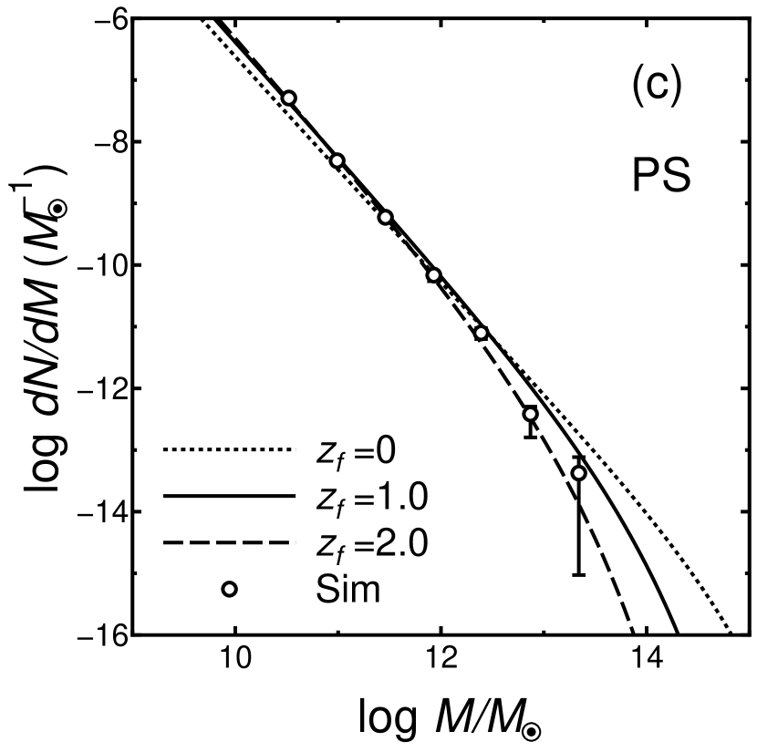
Figure 2: Subhalo mass distribution functions for $z_{f}=0$ or 0.1 (dotted lines), $z_{f}=1.0$ (solid lines), and $z_{f}=2.0$ (dashed lines). (a) $n_{\rm SPS}$, (b) $n_{\rm EPS}$, and (c) $n_{\rm PS}$. The MDF at $z=0$ obtained from the numerical simulation by Okamoto & Habe (1999) is shown by the circles.

We also compare our model with another numerical simulation done by Okamoto & Habe (1999). They adopted cosmological parameters of $\Omega_{0}=1$, $\lambda=0$, $\sigma_{8}=2/3$, $\Gamma=0.5$, and $h=0.5$. The present mass of a cluster is $M_{0}=9.3\times 10^{14}\;M_{\sun}$. In their simulation, the cluster contains one million particles within the final virial radius and is simulated using a force resolution of 5.0 kpc (0.2% of the virial radius). The particle mass is $1.08\times 10^{9}\;M_{\sun}$. Thus, the resolution is a little worse than Ghigna et al. (2000). Figure 2 shows the MDF of subhalos in the cluster. For vertical axes, we use $dN/dM=n_{i}$ ($i=$SPS, EPS, and PS) following Okamoto & Habe (1999). For $z_{f}\gtrsim 1$, the three models are not very different for $M\lesssim 10^{12}\;M_{\sun}$, which is the same as in Figure 1. The result of Okamoto & Habe (1999) at $z=0$ is also shown in Figure 2. As can be seen, $n_{\rm SPS}$ at $z_{f}\sim 2$ is consistent with the MDF of subhalos obtained by Okamoto & Habe (1999). In fact, they indicated that the MDF does not evolve significantly from $z=2$ to the present; this cluster seems to have formed earlier than that in Ghigna et al. (2000). Okamoto & Habe argue that the reason why the MDF in their simulated cluster agrees better with $n_{\rm PS}$ than with $n_{\rm EPS}$ at $z_{f}\sim 2$ may be because of their halo-finding algorithm. However, our results suggest this difference may be because $n_{\rm EPS}$ does not include the effect of spatial correlations of fluctuations and because $n_{\rm PS}$ is almost the same as $n_{\rm SPS}$ at $z_{f}\sim 2$ (Figure 2).

4 Tidal Stripping and Dynamical Friction

We should note that we do not consider some mechanisms that could change the MDF of subhalos in a cluster after the cluster formation; these mechanisms might have been effective even in cluster progenitors.

First, tidal stripping reduces the mass of subhalos. We assume that the density profiles of subhalos and the main cluster are represented by the so-called NFW profile:

$$\rho(r)=\frac{\rho_{0}r_{s}^{3}}{r(r+r_{s})^{2}}\>,$$ (29)

where $r_{s}$ and $\rho_{0}$ are the characteristic radius and density of the halo, respectively (Navarro, Frenk, & White, 1997). The mass profile is given by

$$M(r)=M_{\rm vir}f(x)/f(C)\>,$$ (30)

where

$$f(x)=\ln(1+x)-\frac{x}{1+x}\;,\;\;x=\frac{r}{r_{s}}\>,$$ (31)

and

$$C\equiv\frac{r_{\rm vir}}{r_{s}}\approx 124\left(\frac{M_{\rm vir}}{1h^{-1}\;M_{\sun}}\right)^{-0.084}$$ (32)

(Klypin et al., 1999). In this section, we often refer to subhalos and the main cluster as halos, and represent the total mass of halos by their virial masses $M_{\rm vir}$; their virial radii are represented by $r_{\rm vir}$. The shape of the profile is characterized by the concentration parameter $C$. The circular velocity of a halo at a radius $r$ is defined as $v_{c}(r)=[GM(<r)/r]^{1/2}$. For the NFW profile, the maximum of the circular velocity occurs at $r_{\rm max}\approx 2r_{s}$. and it is given by,

$$v_{\rm peak}=\left[\frac{GM_{\rm vir}}{r_{s}}\frac{f(2)}{2f(C)}\right]^{1/2}\;.$$ (33)

The tidal radius $r_{t}$ of a subhalo with mass $M(r)$ and peak circular velocity $v_{\rm peak}$ moving at a radius $R$ from the center of a cluster with mass $M_{0}(R)$ and peak circular velocity $v_{0}$ is given by the radius at which the gravity force of the subhalo is equal to the tidal force of the main cluster. The radius can be derived by solving the following equation for the tidal radius $r_{t}$:

$$\left(\frac{R}{r_{t}}\right)^{3}\frac{M(r_{t})}{M_{0}(R)}=2-\frac{R}{M_{0}}\frac{\partial M_{0}}{\partial R}\;,$$ (34)

which is equivalent to

$$\frac{f(x_{t})}{f(x_{R})}=\left(\frac{x_{t}}{x_{R}}\right)^{3}\left(\frac{r_{s}v_{0}}{R_{s}v_{\rm peak}}\right)^{2}\left[2-\frac{x_{R}^{2}}{(1+x_{R})^{2}f(x_{R})}\right]\;,$$ (35)

where $x_{t}=r_{t}/r_{s}$, $x_{R}=R/R_{s}$, and $R_{s}$ is scale radius of the cluster (Klypin et al., 1999).

On the other hand, tidal stripping can occur by resonances between the force the subhalo exerts on the dark matter particle and the tidal force by the main cluster. In this case, the tidal radius can be obtained by solving the following equation for the tidal radius:

$$\frac{GM(r_{t})}{r_{t}^{3}}=\frac{GM_{0}(R)}{R^{3}}\;,$$ (36)

which is equivalent to

$$\frac{f(x_{t})}{f(x_{R})}=\left(\frac{x_{t}}{x_{R}}\right)^{3}\left(\frac{r_{s}v_{0}}{R_{s}v_{\rm peak}}\right)^{2}$$ (37)

(Klypin et al., 1999). We take the smaller of the two estimates of $r_{t}$.

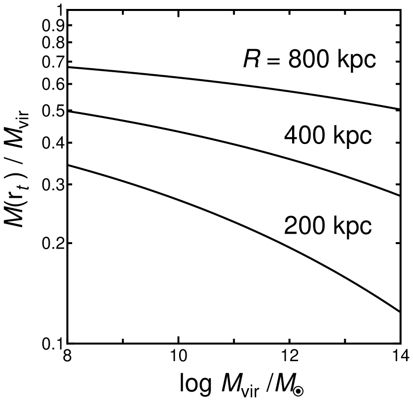
Figure 3: The fraction of mass within the tidal radius of subhalos with different masses for several distances from the cluster center ($R$). The cosmological and cluster parameters are the same as those in Figure 1.

Figure 3 shows the mass fraction of a subhalo within the tidal radius as a function of the ‘subhalo’ virial mass $M_{\rm vir}$. The cosmological and cluster parameters are the same as those in Figure 1. As can be seen, tidal stripping is very effective when the distance from the cluster center is small. Moreover, it is effective when $M_{\rm vir}$ is large, because the concentration parameter $C$ is small (equation [32]). In a real cluster, the effect of tidal stripping depends on the orbit of a subhalo in a cluster. Since it is difficult to discuss the orbits of subhalos analytically, numerical simulations are required to estimate the effect of tidal stripping on entire subhalos in a cluster quantitatively. Ghigna et al. (1998) estimated that for a circular velocity larger than $\sim 10^{2.2}\;\rm km\;s^{-1}$ ($M_{\rm vir}\sim 2.5\times 10^{11}\;M_{\sun}$), the masses of subhalos are smaller than those of isolated halos by $\sim 20-50$% on the average due to tidal stripping. Thus, the tidal stripping would affect the comparison between our numerical model and the results of numerical simulations done in §3, especially for the high mass end of the MDFs.

Second, the most massive subhalos often merge with the central “cD galaxy” via dynamical friction. Thus, we may overestimate the number of these subhalos. The time-scale of dynamical friction can be estimated by using Chandrasekhar’s formula. When the density distribution of a cluster is approximated by an isothermal density distribution, a subhalo with the initial position of $R$ reaches the cluster center in the time of

$$t_{\rm fric} = \frac{1.17}{\ln\Lambda}\frac{R^{2}v_{0}}{GM(r_{t})}$$ (38)

$$= 6.4\times 10^{9}{\rm\;yr}\left(\frac{\ln\Lambda}{5}\right)^{-1}\left(\frac{R}{1\>\rm Mpc}\right)^{2}\left(\frac{v_{0}}{1200\rm\>km\>s^{-1}}\right)\left[\frac{M(r_{t})}{10^{13}\>M_{\sun}}\right]^{-1}\;,$$ (39)

where $\Lambda=R_{c}M_{0}(R)/[RM(t_{t})]$, and $R_{c}$ is the cluster radius (Binney & Tremaine, 1987). Note that the time-scale (equation [39]) is not much different from the one obtained by Klypin et al. (1999) without the approximation of an isothermal distribution.

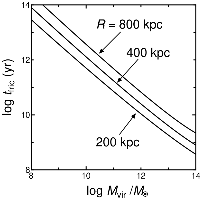
Figure 4: The dynamical friction time for different masses of subhalos for several distances from the cluster center ($R$). The cosmological and cluster parameters are the same as those in Figure 1.

Figure 4 shows the time-scale of dynamical friction $t_{\rm fric}$ as a function of the subhalo virial mass. The cosmological and cluster parameters are the same as those in Figure 1. Massive subhalos near the cluster center are most affected by dynamical friction. The fraction of subhalos that fall into the cluster center depends on the distribution of their orbits. In the numerical simulations done by Ghigna et al. (2000), 60% of subhalos with the circular velocity of $\gtrsim 300\;\rm km\>s^{-1}$ ($M_{\rm vir}\gtrsim 2.5\times 10^{12}\;M_{\sun}$) have merged into the central cD galaxy since $z=3$, although the mergers have been less effective after $z=1$. Thus, the MDFs derived in §3 should be compared with the results of numerical simulations and observations with caution for those massive subhalos.

On the other hand, the distribution of peak circular velocities $v_{\rm peak}$ is less affected by tidal stripping, because the removal of the outer parts of a subhalo does not affect $v_{\rm peak}$ very strongly. Klypin et al. (1999) showed that even if $\sim 70$% of the initial mass of a subhalo is removed by tidal stripping, $v_{\rm peak}$ changes only by $\sim 20$%. Since the numerical simulations done by Ghigna et al. (1998) showed that tidal stripping reduces the mass of massive subhalos at most by $\sim 50$%, the tidal stripping may not affect the distribution function of values of $v_{\rm peak}$ (VDF) for subhalos significantly. Thus, in the next section, we investigate the VDF for subhalos, although the high-velocity end of the VDF may still be affected by dynamical friction, or mergers of subhalos. Observationally, $v_{\rm peak}$ can be obtained more easily than $M$ through the velocity dispersion of stars or the rotation curve of a galaxy. Thus, the VDF is more useful for comparison with observations than the MDF.

5 Velocity Distribution Function

In order to derive the VDF of subhalos from the MDF, we need the relation between the velocity and mass. Since there is no simple analytically derived relation, we use the relation derived by numerical calculations for isolated halos. Navarro, Frenk, & White (1997) found that the relation between $v_{\rm peak}$ and $M$ is

$$v_{\rm peak}=1510\;{\rm km\;s^{-1}}\left(\frac{M}{10^{15}\;M_{\sun}}\right)^{1/3.28}$$ (40)

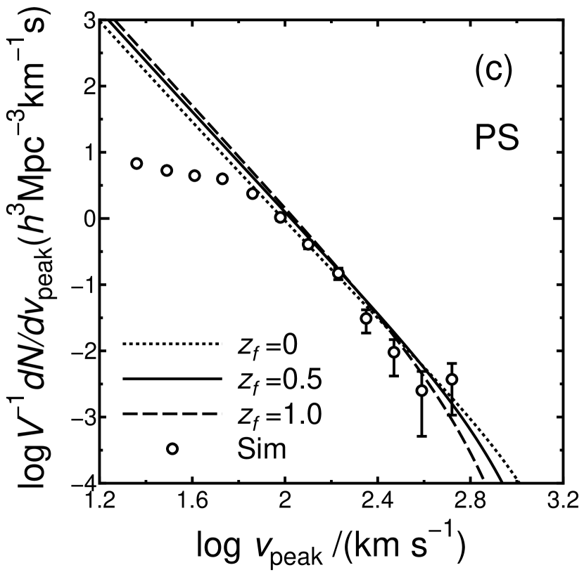
Figure 5: Velocity distribution functions for $z_{f}=0$ or 0.1 (dotted lines), $z_{f}=0.5$ (solid lines), and $z_{f}=1.0$ (dashed lines). (a) $n_{\rm SPS}$, (b) $n_{\rm EPS}$, and (c) $n_{\rm PS}$. The VDF at $z=0$ obtained from the numerical simulation by Ghigna et al. (2000) is shown by the circles.

for the Einstein de-Sitter universe. Although the relation is for $z=0$, it is not much different for $z\lesssim 2$ (Ghigna et al., 1998; Bullock et al., 2001). We assume that this relation holds for subhalos, at least before the collapse of the cluster at $z=z_{f}$. Using equation (40), we transform the MDFs derived in §3 into VDFs; the results are shown in Figure 5. Note that when we discuss the VDFs, $n_{i}$ ($i=$ SPS, EPS, and PS) is a function of $v_{\rm peak}$, and

$$\frac{1}{V}\frac{dN}{dv_{\rm peak}}=\frac{n_{i}}{V}\;.$$ (41)

Since $v_{\rm peak}$ is a monotonically increasing function of $M$, the relation among $n_{\rm SPS}$, $n_{\rm EPS}$, and $n_{\rm PS}$ is the same as that for MDF. In Figure 5, the results of numerical simulations are also shown (Ghigna et al., 2000). In general, $n_{\rm SPS}$ at $z_{f}=0.5$ is consistent the result of numerical calculation as was shown to be the case for the MDF. This may mean that tidal stripping does not significantly affect the MDF of subhalos in the simulated cluster. The deviation of the simulated cluster data from the model at $v_{\rm peak}\lesssim 10^{1.9}\rm\;km\;s^{-1}$ is caused by finite numerical resolution. The slope of the VDF in the simulated cluster is a little steeper than that of $n_{\rm SPS}$ for $v_{\rm peak}\gtrsim 10^{2.3}\rm\;km\;s^{-1}$ if we remove the largest $v_{\rm peak}$ point. This may be caused by mergers of massive subhalos with the central cD galaxy.

If the VDF is not significantly influenced by tidal stripping, we can use it to derive the effective formation redshift of a cluster. Figure 6 shows the observed cumulative number of subhalos in the Virgo cluster derived from galaxy data (Binggeli et al., 1985; Moore et al., 1999) and the integrated $n_{\rm SPS}$ for various $z_{f}$. The cosmological parameters for $n_{\rm SPS}$ are the same as those in Ghigna et al. (2000). The comparison suggests that $z_{f}\sim 2$, although the slope of the Virgo data does not match that of $n_{\rm SPS}$ for $v_{\rm peak}/v_{0}\lesssim 0.1$. Here, $v_{0}$ is the peak velocity $v_{\rm peak}$ of the rotation curve for applicable to the total mass of the cluster. The deviation for low $v_{\rm peak}$ subhalos may be because the corresponding galaxies are too faint to be detected. Note that that the derived formation redshift, $z_{f}\sim 2$, is the redshift at which the growth of subhalos stopped. This corresponds to the time when the potential wells of the cluster progenitors, in which the subhalos were located, became sufficiently deep, even if the progenitors had not yet merged into one cluster. Since the subhalos stopped growing, the formation of galaxies in them is also expected to decrease for $z<z_{f}$. In the irregular Virgo cluster, $z_{f}$ may correspond to the time at which the oldest galaxies were formed, even though the cluster itself is still merging at present.

We note that we cannot rule out the possibility that $z_{f}$ is somewhat smaller than 2 because of the ambiguity of the number and circular velocity of massive subhalos. In general, for massive subhalos, dynamical friction may cause them to merge into one large (cD) galaxy, which reduces their number. However, although there is a moderately large galaxy (M87) at the center of the Virgo cluster, it is not usually classified as a cD galaxy and is probably not the most luminous galaxy in the cluster. Alternatively, the circular velocity of the galaxy residing in a massive subhalo may not represent that of the massive subhalo; the former may be smaller than the latter. In fact, Davis & White (1996) showed that the temperature of diffuse X-ray gas is systematically higher than that of kinetic temperature of stars for bright elliptical galaxies. If the temperature of the X-ray gas is considered to represent the depth of potential well of the halo around the elliptical galaxy, it shows the inconsistency of circular velocity between galaxies and subhalos. Moreover, Matsushita (2001) showed that bright elliptical galaxies with extend X-ray emission tend to have high X-ray temperature compared to those with compact X-ray emission for a given stellar velocity dispersion. On the other hand, the X-ray gas may be affected by other heating processes (e.g., supernovae).

These results suggest the existence of very large, massive subhalos whose X-ray temperature is much higher than kinetic temperature of the stars in the galaxies located in them. Recent Chandra observations have revealed the presence of such massive subhalos in clusters; most of them are moving with the Mach number of $\sim 1$ in clusters without losing their identity. Thus, in the next section, we discuss the relation between the large X-ray subhalos and VDF.

6 Cold Fronts

Large X-Ray subhalos are found in some clusters as low temperature X-ray components with cold fronts (Markevitch et al., 2000; Vikhlinin et al., 2001; Mazzotta et al., 2001, 2002; Sun et al., 2002). The cold fronts are contact interfaces between the cooler gas in the subhalo and the hotter intracluster medium in the main cluster. The ratio of X-ray temperature of the subhalos to that of their host clusters is about $1/2$. Thus, if the X-ray temperature is proportional to $v_{\rm peak}^{2}$, the corresponding velocity ratio is $v_{\rm peak}/v_{0}\sim 1/\sqrt{2}$.

Mazzotta et al. (2001) suggested that a cluster with a large subhalo may be the result of the collapse of two different perturbations in the primordial density field on two different linear scales at nearly the same location in space. As the density field evolves, both perturbations start to collapse. The small-scale perturbation collapses first and forms a large subhalo, and then the larger perturbation collapses and forms a cluster. If the initial position of the subhalo was only slightly offset from the center of the cluster, it would infall into the cluster center with small velocity and oscillate around the cluster center. This would prevent the cool gas in the subhalo from being removed by ram-pressure stripping or the Kelvin-Helmholtz instability. We note that Fujita et al. (2002) showed that the observed subhalos with cold fronts are stable for $0.5-1$ Gyr against large-scale Kelvin-Helmholtz instability.

Therefore, it would be interesting to estimate the probability of finding such large subhalos near centers of clusters, and to compare this probability with the observed rate of occurrence of cold fronts. If we had enough observational data about the massive subhalos, these could be used to study the validity of our MDF or VDF model. However, at present the number of clusters in which large X-ray subhalos are found is too small to allow a detailed discussion of the rate of occurrence of cold fronts. Thus, in this study, we just predict the nature of the massive subhalos, assuming that our model is correct. The cumulative number of the most massive halos is larger for smaller $z_{f}$ (Figure 6), because hierarchical clustering proceeds furthest. Thus, we use $n_{\rm SPS}$ at $z_{f}=0$ to estimate the maximum probability of finding those subhalos.

Figure 6 shows that the cumulative number, $N(0.71<v_{\rm peak}/v_{0}<1)$, is about 0.3, which means that at most one third of clusters should have large subhalos, some of which may have cold fronts similar to the observed ones. In order to find the initial position of the subhalos in a precluster region, we calculate the number by changing the radius, $R$, within which the conditional probability (equation [9]) is averaged. Figure 7 shows the result for the same cluster in Figure 6. Since $N(r<R,0.71<v_{\rm peak}/v_{0}<1)$ is almost constant for $R/R_{0}\gtrsim 0.5$, it is most likely that the initial position of the subhalo is $R/R_{0}\lesssim 0.5$. Because we do not consider the spatial distribution of mass in a precluster region and the detailed evolution of cluster collapse, we cannot exactly predict the infall or oscillating velocity of the subhalo in a cluster. However, if the initial position of the subhalo is well inside the precluster region, the infall or oscillating velocity may be subsonic or at most transonic, which may be consistent with the observations (Markevitch et al., 2000; Vikhlinin et al., 2001; Mazzotta et al., 2001, 2002). Note that if the initial position of a subhalo is near $r=R_{0}$, the Mach number of the infall velocity should be $\sim 2-3$ (Sarazin, 2002). The above result suggests that most of the X-ray substructures in clusters have not fallen in from large distances, as would be true for cluster mergers. Instead, most of the cold fronts may be due to internal subhalos. The fact that clusters having subhalos moving with highly supersonic velocities (e.g. 1E0657$-$56; Markevitch et al., 2002) are rarely found may support this idea, although the number of clusters for which the velocities of subhalos are derived is small.

As is mentioned in §4, the large subhalos should be affected by dynamical friction ($v_{c}\gtrsim 300\;\rm km\>s^{-1}$ according to Ghigna et al. 1998). In approximately the time shown in equation (39) the subhalos reaches the cluster center. If the subhalos are not completely disrupted before they reach the cluster center, the clusters should have a potential well with two different spatial scales. In fact, Ikebe et al. (1996) found a double dark halo distribution in the Fornax cluster. On the other hand, in the central regions of many clusters, cool gas is observed (Fabian, 1994). These subhalos may provide cool gas into the cluster center.

7 Conclusions

We have constructed a model of the mass distribution function (MDF) of subhalos in clusters, including the fact that the subhalos grew from spatially correlated density fluctuations in high-density regions. If a cluster forms at a low redshift, the derived mass distribution function of subhalos is intermediate between the Press-Schechter mass distribution function and a conditional mass distribution function derived by an extension of the PS formalism. However, if a cluster forms at high redshift, our subhalo MDF is nearly identical to these other MDFs for low mass subhalos. The velocity distribution functions show similar trends. We compare our model MDF with the results of $N$-body numerical simulations. We find that they are consistent with each other. The comparison of our model with the subhalo population derived from galaxy data suggests that the subhalos in Virgo cluster stopped growing at $z\sim 2$. Our model predicts that at most 1/3 of clusters should have large X-ray subhalos like the ones observed as cold fronts with Chandra. Many of the observed X-ray substructures in clusters may not be the result of cluster mergers; instead, they may be due to internal substructures within the clusters.

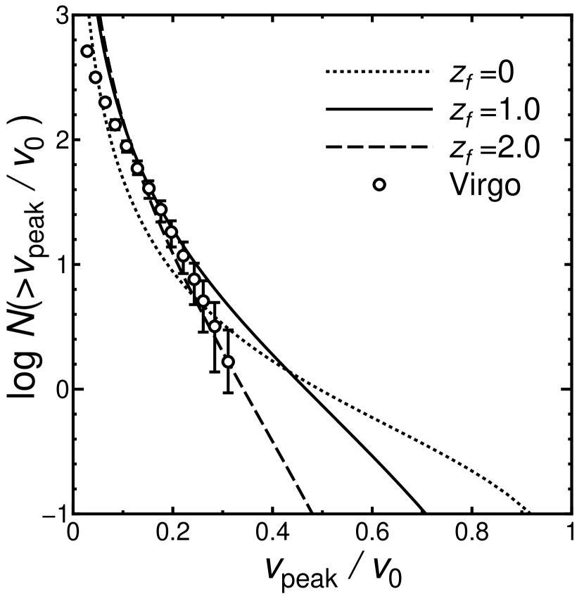
Figure 6: Circles show the observed cumulative number of subhalos in the Virgo cluster derived from galaxy observations (Binggeli et al., 1985; Moore et al., 1999). The lines give the integrated SPS MDF for $z_{f}=0$ or 0.1 (dotted lines), $z_{f}=1.0$ (solid lines), and $z_{f}=2.0$ (dashed lines). The integrated SPS MDF was calculated using the cosmological parameters in Ghigna et al. (2000).

Figure 7: The average number of subhalos with $0.71<v_{\rm peak}/v_{0}<1$ within $r<R$. We assume that $z_{f}=0$.

References

- Binggeli et al. (1985) Binggeli, B., Sandage, A., & Tammann, G. A. 1985, AJ, 90, 1681
- Binney & Tremaine (1987) Binney, J. & Tremaine, S. 1987, Galactic Dynamics, (Princeton: Princeton Univ. Press), 428
- Bond et al. (1991) Bond, J. R., Cole, S., Efstathiou, G., & Kaiser, N. 1991, ApJ, 379, 440
- Bower (1991) Bower, R. G. 1991, MNRAS, 248, 332
- Bullock et al. (2001) Bullock, J. S., Kolatt, T. S., Sigad, Y., Somerville, R. S., Kravtsov, A. V., Klypin, A. A., Primack, J. R., & Dekel, A. 2001, MNRAS, 321, 559
- Davis & White (1996) Davis, D. S. & White, R. E. 1996, ApJ, 470, L35
- Fabian (1994) Fabian, A. C. 1994, ARA&A, 32, 277.
- Fujita et al. (2002) Fujita, Y., Sarazin, C. L., Kempner, J. C., Rudnick, L., Slee, O. B. 2002, Roy, A. L., Andernach, H., & Ehle, M. 2002, ApJ, in press (astro-ph/0204188)
- Fukushige & Makino (2001) Fukushige, T. & Makino, J. 2001, ApJ, 557, 533
- Ghigna et al. (1998) Ghigna, S., Moore, B., Governato, F., Lake, G., Quinn, T., & Stadel, J. 1998, MNRAS, 300, 146
- Ghigna et al. (2000) Ghigna, S., Moore, B., Governato, F., Lake, G., Quinn, T., & Stadel, J. 2000, ApJ, 544, 616
- Colín et al. (1999) Colín, P., Klypin, A. A., Kravtsov, A. V., & Khokhlov, A. M. 1999, ApJ, 523, 32
- Gottlöber et al. (2001) Gottlöber, S., Klypin, A., & Kravtsov, A. V. 2001, ApJ, 546, 223
- Ikebe et al. (1996) Ikebe, Y. et al. 1996, Nature, 379, 427
- Jing & Suto (2000) Jing, Y. P. & Suto, Y. 2000, ApJ, 529, L69
- Klypin et al. (1999) Klypin, A., Gottlöber, S., Kravtsov, A. V., & Khokhlov, A. M. 1999, ApJ, 516, 530
- Lacey & Cole (1993) Lacey, C. & Cole, S. 1993, MNRAS, 262, 627
- Markevitch et al. (2000) Markevitch, M. et al. 2000, ApJ, 541, 542
- Markevitch et al. (2002) Markevitch, M., Gonzalez, A. H., David, L., Vikhlinin, A., Murray, S., Forman, W., Jones, C., & Tucker, W. 2002, ApJ, 567, L27
- Matsushita (2001) Matsushita, K. 2001, ApJ, 547, 693
- Mazzotta et al. (2001) Mazzotta, P., Markevitch, M., Vikhlinin, A., Forman, W. R., David, L. P., & VanSpeybroeck, L. 2001, ApJ, 555, 205
- Mazzotta et al. (2002) Mazzotta, P., Markevitch, M., Forman, W. R., Jones, C., Vikhlinin, A., David, L. P., & VanSpeybroeck, L. 2002, ApJ, submitted (astro-ph/0108476)
- Moore et al. (1999) Moore, B., Ghigna, S., Governato, F., Lake, G., Quinn, T., Stadel, J., & Tozzi, P. 1999, ApJ, 524, L19
- Moore et al. (1996) Moore, B., Katz, N., & Lake, G. 1996, ApJ, 457, 455
- Nagashima (2001) Nagashima, M. 2001, ApJ, 562, 7
- Navarro et al. (1997) Navarro, J. F., Frenk, C. S., & White, S. D. M. 1997, ApJ, 490, 493
- Okamoto & Habe (1999) Okamoto, T. & Habe, A. 1999, ApJ, 516, 591
- Press & Schechter (1974) Press, W. H. & Schechter, P. 1974, ApJ, 187, 425
- Sarazin (2002) Sarazin, C. L. 2002, in Merging Processes in Clusters of Galaxies, ed. L. Feretti, I. M. Gioia, & G. Giovannini (Dordrecht: Kluwer), in press (astro-ph/0105418)
- Sun et al. (2002) Sun, M., Murray, S. S., Markevitch, M., & Vikhlinin, A. 2002, ApJ, in press (astro-ph/0103103)
- Tormen et al. (1998) Tormen, G., Diaferio, A., & Syer, D. 1998, MNRAS, 299, 728
- Vikhlinin et al. (2001) Vikhlinin, A., Markevitch, M., & Murray, S. S. 2001, ApJ, 551, 160
- White et al. (2001) White, M., Hernquist, L., & Springel, V. 2001, ApJ, 550, L129
- Yano et al. (1996) Yano, T., Nagashima, M., & Gouda, N. 1996, ApJ, 466, 1