Three-Dimensional Mapping of the Dark Matter

Abstract

We study the prospects for three-dimensional mapping of the dark matter to high redshift through the shearing of faint galaxies images at multiple distances by gravitational lensing. Such maps could provide invaluable information on the nature of the dark energy and dark matter. While in principle well-posed, mapping by direct inversion introduces exceedingly large, but usefully correlated noise into the reconstruction. By carefully propagating the noise covariance, we show that lensing contains substantial information, both direct and statistical, on the large-scale radial evolution of the density field. This information can be efficiently distilled into low-order signal-to-noise eigenmodes which may be used to compress the data by over an order of magnitude. Such compression will be useful for the statistical analysis of future large data sets. The reconstructed map also contains useful information on the localization of individual massive dark matter halos, and hence the dark energy from halo number counts, but its extraction depends strongly on prior assumptions. We outline a procedure for maximum entropy and point-source regularization of the maps that can identify alternate reconstructions.

I Introduction

Embedded within the evolution of the three-dimensional distribution of the dark matter lies a wealth of information on the nature of the dark energy and dark matter in the universe. The growth of its clustering in volumes associated with redshift, along with the abundance of discrete dark matter clumps or halos which it controls, is one of our most direct probes of the expansion history (e.g. deprobes ). It is certainly the one that is best understood from the theoretical standpoint.

Unfortunately, most probes of structure in the low redshift universe rely on luminous matter, e.g. galaxies and clusters of galaxies, as tracers of dark matter distribution. Such probes are subject to significant uncertainties in the physical processes that govern the formation and evolution of the tracers. The only exception is the image distortion from gravitational lensing of distant objects by the dark matter. On large scales and for small distortions, this is known as weak gravitational lensing weak ; weaklss . The distortion of faint galaxy images by the large-scale structure of the universe has now been detected with high significance by several experimental groups weakdet .

A fundamental obstacle for weak lensing studies of the matter distribution is that the technique is inherently two-dimensional. All of the matter along the line-of-sight to a distant source contributes to lensing and so the distortion reflects a two-dimensional projection of the dark matter. Unfortunately then the evolution of structure is hidden in the missing radial dimension. This limitation can in principle be overcome by a tomographic reconstruction of the three-dimensional distribution from sources spanning a range of distances or redshifts.

Under fairly restrictive assumptions, this tomographic technique has been applied to lensing data to localize the halo associated with a cluster of galaxies Witetal01 and validated by follow-up studies. The critical assumption is that the lensing mass be a single halo, well localized in redshift. Taylor Tay01 has recently shown that these and other restrictions are unnecessary in principle. In the absence of noise, tomographic mapping of the dark matter is a well-posed problem. In this paper, we study the feasibility of reconstructing three-dimensional dark matter maps in the presence of noise. We will show that a careful accounting of the noise and in particular its covariance across the map is essential for extracting information from the map.

Tomography also presents a severe data analysis challenge, similar to but potentially far worse than that facing cosmic microwave background (CMB) experiments. A full weak lensing data set will have a two-component, two-dimensional megapixel map for each of ten or more source redshift slices. We also study how techniques developed for the CMB and galaxy redshift surveys may be applied to compress these data to a more manageable size.

The outline of the paper is as follows. We begin in § II with a brief review of mapmaking techniques and apply them to the two-dimensional lensing observables keeping careful track of the propagation of measurement errors. We use these techniques to reconstruct the three-dimensional distribution of the dark matter in § III. Although the reconstruction is extremely noisy for any realistic situation, the noise has very particular properties that are absent in the signal. This fact is used to regularize the solution and radically compress the data in the large-scale structure regime in § IV, and in the individual dark matter halo regime in § V. We discuss these results in § VI.

II Formalism

We begin by briefly reviewing general mapmaking techniques in § II.1, establishing notation used throughout the paper. These techniques are then applied to the two-dimensional weak lensing shear in § II.2 for the reconstruction of convergence maps. The latter follows the well-known Kaiser & Squires KaiSqu93 algorithm but we pay special attention to the propagation of noise into the convergence reconstruction as that will play a central role in the three-dimensional mapping that follows. In § II.3, we discuss the generalization to multiple source planes.

II.1 Mapmaking

Mapmaking can be formulated in terms of the general inverse problem Teg97 , where we seek an estimate $\hat{\bf s}_{a}$ of a signal vector ${\bf s}_{a}$ from a data vector ${\bf d}_{b}$ that is a linear projection ${\bf P}_{ba}$ of the signal plus measurement noise ${\bf n}_{b}$,

$${\bf d}_{b}={\bf P}_{ba}{\bf s}_{a}+{\bf n}_{b}\,.$$ (1)

The projection matrix ${\bf P}_{ba}$ has dimensions ($n_{b}$,$n_{a}$), the number of elements in the data and signal vectors respectively, and hence need not be square. Here and below subscripts are labels and not elements of the vectors and matrices; elements will be denoted by $[{\bf P}_{ba}]_{ij}$. We assume that both the signal and the noise have zero mean $\langle{\bf s}_{a}\rangle=\langle{\bf n}_{b}\rangle=0$, that the signal and noise are uncorrelated, $\langle{\bf s}_{a}{\bf n}_{b}^{t}\rangle=0$, and that the noise covariance is known,

$${\bf N}_{bb}\equiv\langle{\bf n}_{b}{\bf n}_{b}^{t}\rangle\,.$$ (2)

The statistical properties of the signal,

$${\bf S}_{aa} \equiv \langle{\bf s}_{a}{\bf s}_{a}^{t}\rangle\,,$$ (3)

may or may not be known.

The estimated signal $\hat{\bf s}_{a}$ is that which minimizes

$$\chi^{2}+H\,,$$ (4)

where

$$\chi^{2}=({\bf d}_{b}-{\bf P}_{ba}\hat{\bf s}_{a})^{t}{\bf N}_{bb}^{-1}({\bf d}_{b}-{\bf P}_{ba}\hat{\bf s}_{a})\,.$$ (5)

and the penalty function $H$ is a set of constraints and/or a regularization to choose among degenerate solutions.

Minimizing $\chi^{2}$ (with $H=0$) returns the linear estimator

$$\hat{\bf s}_{a}={\bf R}_{ab}{\bf d}_{b}\,,$$ (6)

where

$${\bf R}_{ab}=[{\bf P}_{ba}^{t}{\bf N}_{bb}^{-1}{\bf P}_{ba}]^{-1}{\bf P}_{ba}^{t}{\bf N}_{bb}^{-1}\,,$$ (7)

and this simple reconstruction is well-posed as long as the product in square brackets is invertible. If ${\bf P}_{ba}$ itself is invertible then ${\bf R}_{ab}={\bf P}_{ba}^{-1}$ and the estimator becomes independent of both the signal and the noise. The errors in the reconstruction,

$$\hat{\bf s}_{a}-{\bf s}_{a}=[{\bf R}_{ab}{\bf P}_{ba}-{\bf I}]{\bf s}_{a}+{\bf R}_{ab}{\bf n}_{b}\,,$$ (8)

imply a new noise covariance

$${\bf N}_{aa} \equiv \langle(\hat{\bf s}_{a}-{\bf s}_{a})(\hat{\bf s}_{a}-{\bf s}_{a})^{t}\rangle$$ (9)

$$= [{\bf P}_{ba}^{t}{\bf N}_{bb}^{-1}{\bf P}_{ba}]^{-1}\,,$$

which is independent of the signal. Note that minimizing $\chi^{2}$ is not the same as minimizing the reconstruction noise ${\bf N}_{aa}$ since reconstruction errors are not penalized by $\chi^{2}$ in the noise-dominated regime. In fact, it minimizes ${\bf N}_{aa}$ subject to the constraint ${\bf R}_{ab}{\bf P}_{ba}={\bf I}$ Teg97 .

For a noisy reconstruction, prior knowledge of the statistical properties of the signal can be used as to set a penalty function for a new estimator of the signal

$$H=\hat{\bf s}_{w}^{t}{\bf S}_{aa}^{-1}\hat{\bf s}_{w}\,.$$ (10)

Minimization of Eqn. (4) then returns the Wiener filtered estimate of the signal $\hat{\bf s}_{w}={\bf R}_{wb}{\bf d}_{b}$, where

$${\bf R}_{wb} = [{\bf S}_{aa}^{-1}+{\bf P}_{ba}^{t}{\bf N}_{bb}^{-1}{\bf P}_{ba}]^{-1}{\bf P}_{ba}^{t}{\bf N}_{bb}^{-1}$$ (11)

$$= {\bf S}_{aa}{\bf P}_{ba}^{t}[{\bf P}_{ba}{\bf S}_{aa}{\bf P}_{ba}^{t}+{\bf N}_{bb}]^{-1}\,,$$

which has the heuristic form of signal/(signal+noise) and so suppresses the signal in the noise-dominated regime. The estimator $\hat{\bf s}_{w}$ has the noise properties

$${\bf N}_{ww} = [{\bf R}_{wb}{\bf P}_{ba}-{\bf I}]{\bf S}_{aa}[{\bf R}_{wb}{\bf P}_{ba}-{\bf I}]^{t}$$ (12)

$$\quad+{\bf R}_{wb}{\bf N}_{bb}{\bf R}_{wb}^{t}\,.$$

The Wiener estimator may alternately be derived as that which minimizes ${\bf N}_{ww}$ Teg97 .

For a well-posed inverse problem the minimum-$\chi^{2}$ and Wiener reconstructions are related by an invertible operation. We can view the result of the former as providing a new data vector ${\bf d}_{a}=\hat{\bf s}_{a}$ having noise ${\bf n}_{a}$ with a covariance ${\bf N}_{aa}$. Then with the model of the data ${\bf d}_{a}={\bf I}\ {\bf s}_{w}+{\bf n}_{a}$, Eqn. (11) for the Wiener filter returns

$$\hat{\bf s}_{w}={\bf R}_{wa}{\bf d}_{a}={\bf R}_{wa}\hat{\bf s}_{a}\,,$$ (13)

where

$${\bf R}_{wa}={\bf S}_{aa}[{\bf S}_{aa}+{\bf N}_{aa}]^{-1}\,.$$ (14)

Since this matrix is invertible, the two reconstructions are formally equivalent.

Because the minimum-$\chi^{2}$ method does not require prior knowledge, we choose it as the primary mapping technique if the inverse problem is well-posed. Alternatively, for an ill-posed inverse problem, where the matrix ${\bf P}_{ba}^{t}{\bf N}_{bb}^{-1}{\bf P}_{ba}$ is not invertible, Wiener filtering can serve as the primary technique.

As the Wiener example implies, secondary processing operations on the primary map can be viewed as simply another round of mapmaking. Any linear operation that is invertible will retain the same information content as the original so long as the noise covariance is properly propagated. We will use this technique to go from the observed lensing shear to the convergence to the density field and finally to the Wiener, signal-to-noise, or point source filtered density fields.

II.2 Lensing Observables

The distortion of images due to weak gravitational lensing is described by the Jacobian matrix of the mapping between the two-dimensional source and image planes (e.g. BarSch01 )

$${\bf A}=\left(\begin{array}[]{cc}1-\kappa-\gamma_{1}&-\gamma_{2}\\ -\gamma_{2}&1-\kappa+\gamma_{1}\end{array}\right)\,,$$ (17)

where all components are functions of position on the sky $\hat{\bf n}$.

The galaxy ellipticities form a noisy estimator of the shear components $(\gamma_{1},\gamma_{2})$ which are in turn related to the convergence $\kappa$ by (e.g. BarSch01 )

$$[\gamma_{1}\pm i\gamma_{2}](\hat{\bf n})=-\frac{1}{\pi}\int d\hat{\bf n}^{\prime}\frac{e^{\pm 2i\phi}}{\theta^{2}}\kappa(\hat{\bf n}^{\prime})\,,$$ (18)

where $\theta\equiv|\hat{\bf n}-\hat{\bf n}^{\prime}|$ denotes the length of the pixel separation vector, and $\phi$ denotes its azimuthal angle in the coordinate system that defines the shear components. By constructing a map of $\kappa$ from the shear data, one compresses the data set by a factor of two and also transforms the data into a form that is more conveniently related to the three-dimensional density field (see § III).

Discretizing the sky into pixels returns Eqn. (18) in the form of the general mapmaking problem of Eqn. (1), where the signal ${\bf s}_{\kappa}$ has been linearly projected onto the data space with measurement noise added to form the data vector, ${\bf d}_{\gamma}$. Explicitly, if one orders the data vector as

$${\bf d}_{\gamma}=\{\gamma_{1}(\hat{\bf n}_{1}),\gamma_{2}(\hat{\bf n}_{2});\ldots;\gamma_{1}(\hat{\bf n}_{n_{\rm pix}}),\gamma_{2}(\hat{\bf n}_{n_{\rm pix}})\}\,,$$ (19)

the model becomes

$${\bf d}_{\gamma}={\bf P}_{\gamma\kappa}{\bf s}_{\kappa}+{\bf n}_{\gamma}\,,$$ (20)

with the projection matrix

$$\left[{\bf P}_{\gamma\kappa}\right]_{(2i-1)j} = -\frac{A_{j}}{\pi}\frac{\cos 2\phi_{ij}}{\theta^{2}_{ij}}\,,$$

$$\left[{\bf P}_{\gamma\kappa}\right]_{(2i)j} = -\frac{A_{j}}{\pi}\frac{\sin 2\phi_{ij}}{\theta^{2}_{ij}}\,,$$ (21)

where the indices run over the pixels of area $A_{j}$ and the angles are defined as averages over the pixel.

If the noise in the shear data is dominated by the intrinsic ellipticity of galaxies, it is given by

$$[{\bf N}_{\gamma\gamma}]_{ij}=[{\bf I}]_{ij}\frac{\gamma_{\rm rms}^{2}}{[{\bf n}_{\rm gal}]_{i}}\,,$$ (22)

where ${\bf n}_{\rm gal}$ is a vector containing the number of galaxies per pixel. Here $\gamma_{\rm rms}$ is the rms error from intrinsic ellipticities and measurement errors per galaxy. The intrinsic alignment of galaxies on small scales is a potential source of correlated noise intrinsic . While we neglect its currently uncertain contribution here, the framework we establish can handle any source of noise provided its covariance is known.

We have implicitly assumed here a single set of shear data per pixel. If the full data set includes multiple observations of the shear of varying quality or even simply the unbinned individual galaxy estimates themselves, one merely extends the data vector and the mapmaking algorithm combines them with the appropriate noise weighting. Mapmaking can also test the validity of Eqn. (18), or more properly the data model of Eqn. (20), through a reconstruction of the complementary “B-mode” map. This procedure amounts to multiplying the kernel in Eqn. (18) by $i$ corresponding to a rotation of the shear vectors by $45^{\circ}$. The reconstructed map should be consistent with noise.

The estimator of $\kappa$ and its noise properties then follow from Eqns. (6) and (9) aside from two subtleties. The first subtlety involves the so-called mass-sheet degeneracy: adding a constant to the $\kappa$ signal in Eqn. (18) yields no effect in the shear data. There is then a singular value associated with the inversion in Eqn. (7). In general, one way to handle unconstrained modes is to add them to the data vector and assign them zero value but a large noise variance unconst . The covariance matrix of Eqn. (9) then properly accounts for the lack of information on these modes. For the mass-sheet degeneracy, one appends: a zero to the data vector in Eqn. (19); a row to the projection matrix with uniform elements $1/n_{\rm pix}$; and a diagonal entry to the noise matrix Eqn. (22) with a value substantially greater than the variance of $\kappa$ smoothed across the field size in any reasonable cosmology.

This same procedure applies to the second subtlety. Since Eqn. (18) represents a convolution, the discrete representation is formally ill-defined for non-contiguous regions of the data, including holes and edges of the finite field. The sharp fall-off of the convolution kernel implies that only neighboring regions will be affected. Again one can account for these problems by assigning to the unmeasured or contaminated regions zero signal but a substantially larger noise variance than either the signal or noise in the neighboring measured region. The mapping procedure then propagates an appropriately large and correlated noise into the reconstruction. If the gaps in the data are comparable to the contiguous regions, then Wiener filtering should serve as the primary mapping technique.

In the limit of infinitesimal pixels and an infinite contiguous field both these subtleties disappear and

$${\bf P}_{\gamma\kappa}^{t}{\bf P}_{\gamma\kappa}\rightarrow{\bf I}\,.$$ (23)

So if the noise in the shear is also uncorrelated and statistically homogeneous, ${\bf N}_{\gamma\gamma}\propto{\bf I}$ and Eqn. (6) becomes

$$\hat{\bf s}_{\kappa}\rightarrow{\bf P}_{\gamma\kappa}^{t}{\bf d}_{\gamma}\,,$$ (24)

which is the discrete form of the Kaiser & Squires KaiSqu93 result. Furthermore, the noise in the $\kappa$ reconstruction ${\bf N}_{\kappa\kappa}\rightarrow{\bf N}_{\gamma\gamma}$. We will use this approximation for illustration purposes. These limiting behaviors and their mapmaking implications are simplest to derive in the Fourier domain (e.g. Sel98 ).

II.3 Multiple Source Planes

So far we have implicitly assumed a single source plane for the lensing observables. In reality the source galaxies will be broadly distributed around some median set by the depth of the survey. It is this fact that makes three-dimensional mapping possible.

For definiteness we will typically assume a median redshift $z_{\rm med}=1$ and a functional form Kai98

$$\frac{dN}{dz}=A\frac{dD}{dz}D\exp[-(D/D_{*})^{4}]\,,$$ (25)

where $D$ is the comoving distance in the fiducial cosmological model, and $D_{*}$ is set to reproduce the median redshift. The normalization constant $A$ is chosen to match the number density of faint galaxies on the sky. We will take $\bar{n}=3.6\times 10^{5}$ deg^-2 and $\gamma_{\rm rms}=0.3$ for illustration purposes; this represents an estimate of the usable galaxies and the shear noise per galaxy measured from a space-based platform (A. Refregier, private communication).

To separate the source galaxies into redshift bins, galaxy redshifts with errors that are smaller than the bin size are needed. Without spectroscopic redshifts, the precision will be limited by photometric techniques. We will take a minimum redshift bin of $\Delta z=0.025$ to test the potential of future surveys. Current surveys return photometric redshifts with $\Delta z\approx 0.06$ Witetal01 . We shall see that reconstruction noise due to the finite number of galaxies per bin dominates before this resolution is reached so that the photometric redshift errors of even current surveys are unlikely to be the limiting source of error.

The mapmaking technique for multiple source planes with independent noise, as is appropriate for the intrinsic ellipticity noise of Eqn. (22), is the trivial generalization of a single source plane. With correlated noise in the shear from systematic effects or intrinsic galaxy alignments, one forms a data vector of all the observations and applies the same mapmaking algorithm to estimate $\kappa$ in source redshift bins with appropriately correlated noise.

III Three-Dimensional Mapping

Given two-dimensional convergence maps in multiple source planes, it is in principle possible to reconstruct full three-dimensional density maps (e.g. Tay01 ). We shall see that in practice true mapping requires a prohibitively high signal-to-noise ratio in the lensing observables for reasons fundamental to the lensing projection. We focus here on the radial reconstruction in a single angular pixel since the full three-dimensional distribution may be constructed as a collection of such reconstructions.

III.1 Radial Mapmaking

We now take as the data vector ${\bf d}_{\kappa}$ in $n_{z}$ source redshift bins (in a given angular pixel) and assume that its noise properties ${\bf N}_{\kappa\kappa}$ are defined by the reconstruction in § II.2. The model for the convergence $\kappa$ is a radial projection of the three-dimensional density distribution (e.g. BarSch01 )

$$\kappa(z_{s})=\frac{3}{2}H_{0}^{2}\Omega_{m}\int_{0}^{z_{s}}dz\,\frac{dD}{dz}\,\frac{(D_{s}-D)D}{D_{s}}\,{{\Delta}}\,,$$ (26)

where $D$ is the comoving distance in a flat universe, subscript $s$ denotes evaluation at the redshift of the source $z_{s}$, and ${\Delta}=\delta/a$ is the density fluctuation with the growth rate in a matter-dominated universe scaled out. Discretizing Eqn. (26) in redshift bins returns the general equation of mapmaking (see Eqn. (1))

$${\bf d}_{\kappa}={\bf P}_{\kappa{\Delta}}{\bf s}_{{\Delta}}+{\bf n}_{\kappa}\,,$$ (27)

with

$$[{\bf P}_{\kappa{\Delta}}]_{ij}=\begin{cases}\frac{3}{2}H_{0}^{2}\Omega_{m}{\delta\!D}_{j}\frac{(D_{i+1}-D_{j})D_{j}}{D_{i+1}}&\text{ $D_{i+1}>D_{j}$ },\\ 0&\text{ $D_{i+1}\leq D_{j}$ },\end{cases}$$ (28)

where ${\delta\!D}_{j}$ is the width of bin $j$, the distances are measured to the center of the bins, and we have offset the source redshift bins by 1 so that the projection matrix is purely lower triangular. For notational simplicity we have assumed that the binning in the signal and data space is the same, but the generalization is straightforward.

The reconstructed density field is then given by the general mapmaking equation

$$\hat{\bf s}_{\Delta}={\bf R}_{\Delta\kappa}{\bf d}_{\kappa}\,,$$ (29)

where

$${\bf R}_{\Delta\kappa} = {\bf N}_{\Delta\Delta}{\bf P}_{\kappa\Delta}^{t}{\bf N}_{\kappa\kappa}^{-1}\,.$$ (30)

Here

$${\bf N}_{\Delta\Delta}=[{\bf P}_{\kappa\Delta}^{t}{\bf N}_{\kappa\kappa}^{-1}{\bf P}_{\kappa\Delta}]^{-1}\,,$$ (31)

is the noise covariance of the estimator.

As noted by Taylor Tay01 , the reconstruction is in principle well-posed and does not require regularization if the density field is to be recovered to the same redshift resolution and range as the convergence data. Our more general treatment accounts for inhomogeneities and correlation in the noise, and even gaps in the data (see § II.2). More importantly, it returns the noise covariance of the estimator. We shall see in the next section that without knowledge of the noise covariance the reconstructed density field cannot be used for any practical purpose.

The multipixel generalization of radial mapmaking concatenates the vectors for each pixel. For uncorrelated noise in $\kappa$-pixels, the result is simply the application of mapmaking pixel-by-pixel since the noise matrix is then block diagonal in the pixels. For correlated noise, the noise matrices in the multipixel generalization of Eqns. (30) and (31) couple neighboring pixels.

III.2 Noise Properties

To get a feel for the properties of the reconstruction, consider an idealization with redshift bins that are equal in comoving width ${\delta\!D}$, and noise in $\kappa$ that is both uncorrelated and homogeneous. Then

$${\bf P}_{\kappa\Delta} = C{\bf M}\,,$$

$${\bf N}_{\kappa\kappa} = \sigma^{2}{\bf I}\,,$$ (32)

where

$$C=\frac{3}{2}(H_{0}{\delta\!D})^{2}\Omega_{m}\,,$$ (33)

and

$$[{\bf M}]_{ij}=\begin{cases}(i+1-j)\frac{2j-1}{2i+1}&\text{ $j<i+1$ }\,,\\ 0&\text{ else }\,.\end{cases}$$ (34)

With these simplifications the reconstruction matrix is

$$[{\bf R}_{\Delta\kappa}]_{ij}=\frac{1}{C}\,\frac{2j-1}{2i-1}\times\begin{cases}1&\text{ $j=i-2,i$ }\,,\\ -2&\text{ $j=i-1$ }\,,\\ 0&\text{ else }\,.\end{cases}$$ (35)

Note that the projection matrix is lower triangular, and the reconstruction matrix is tridiagonal.

For $i\gg 1$ the reconstructed density field is essentially the finite difference approximation of the second derivative of the convergence data; this is the same second derivative seen in Taylor’s continuous method Tay01 . To understand this result, consider the response in $\kappa$ to a density fluctuation in a single redshift bin (also see Fig. 5b). As we move out in redshift, the $\kappa$ response is zero until we reach the density fluctuation. As we cross the fluctuation $\kappa$ undergoes a sudden “acceleration,” and thereafter grows slowly. With perfect data, one would identify density fluctuations as regions where the second derivative of $\kappa$ is large. The problem is that the $\kappa$ response accelerates from zero and hence will be hidden by noise locally. This is the fundamental limitation of weak lensing tomography with real data.

Taking finite differences of the data amplifies the noise and strongly correlates it between neighboring pixels. For $i\gg 1$ the noise matrix is

$$[{\bf N}_{\Delta\Delta}]_{ij}=\frac{\sigma^{2}}{C^{2}}\times\begin{cases}1&\text{ $j=i-2,\,i+2$}\,,\\ -4&\text{ $j=i-1,\,i+1$}\,,\\ 6&\text{ $j=i$ }\,,\\ 0&\text{ else }\,.\end{cases}$$ (36)

The noise covariance has a very particular form, which corresponds to a finite-difference approximation of a fourth derivative (see Fig. 1b). That the noise is correlated in this specific way will turn out to be crucial in extracting any information from the reconstruction.

To see this, consider a toy model where the galaxies are equally distributed among $n_{z}$ redshift bins that extend to a cosmologically interesting distance $\Omega_{m}^{1/2}H_{0}D_{\rm max}=1$. Then $\sigma^{2}=n_{z}\gamma_{\rm rms}^{2}/n_{\rm gal}$ and $\Omega_{m}^{1/2}H_{0}{\delta\!D}=n_{z}^{-1}$, and the rms noise per bin in the reconstruction is

$$\sqrt{6}\frac{\sigma}{C}\approx 1.5\left(\frac{n_{z}}{20}\right)^{5/2}\left(\frac{n_{\rm gal}}{3.6\times 10^{5}}\right)^{-1/2}\left(\frac{\gamma_{\rm rms}}{0.3}\right)\,,$$ (37)

where we have scaled the result with numbers from § II.3 for degree scale pixels. Even with these generous assumptions, the signal-to-noise per bin in the reconstruction is generally small and only approaches unity for density fluctuations that approach unity when averaged over these large volumes.

Notice that the noise per bin scales as $n_{z}^{5/2}$, which seems to suggest that increasing the radial resolution decreases the total signal-to-noise ratio. But that would be true only if the noise were uncorrelated. Instead, the fact that the noise covariance has a very specific form that is not seen in realistic signals allows it to be filtered out. The blind reconstruction of primary mapmaking is therefore useful only as a first step in the process. To extract information out of the map, one must regularize the reconstruction with a prior assumption about the signal that is to be recovered.

IV Large-Scale Structure

For scales greater than about $10^{\prime}$ and the depths reached by modern surveys, the convergence field in a typical region of sky is dominated by large-scale structures in the underlying dark matter density field weaklss . Moreover, the fluctuations are in the linear to quasilinear regime where theoretical modeling can be expected to give a good prior assumption about the statistics of the field (§ IV.1). In this limit, one can quantify and better represent the information contained in the noisy three-dimensional density map obtained from the primary mapmaking of the previous section. We apply two well-known techniques: Wiener filtering (§ IV.3) to represent the map itself, and the Karhunen-Loeve transform (§ IV.4) whose eigenmodes encapsulate and expose the underlying information contained in the map.

IV.1 Signal Matrix

In the linear regime, the signal matrix ${\bf S}_{{\Delta}{\Delta}}$ is related to the linear power spectrum as follows. The average density fluctuation within the $i$th redshift window $W_{i}({\bf x})$ becomes

$$\Delta_{i}=a_{i}^{-1}\int d^{3}x\,W_{i}({\bf x})\delta({\bf x})\,,$$ (38)

where $\delta({\bf x})$ is the density fluctuation field. We assume that the windows are normalized so that $\int d^{3}x\,W_{i}=1$. The signal covariance of these density averages is

$$\left[{\bf S}_{\Delta\Delta}\right]_{ij} = \int d^{3}x_{i}\int d^{3}x_{j}\,W_{i}({\bf x}_{i})W_{j}({\bf x}_{j})$$

$$\quad\times\langle\delta({\bf x}_{i})\delta({\bf x}_{j})\rangle$$

$$= \frac{G_{i}}{a_{i}}\frac{G_{j}}{a_{j}}\int\frac{d^{3}k}{(2\pi)^{3}}W_{i}({\bf k})W_{j}^{*}({\bf k})P(k)\,,$$

where $P(k)$ is the linear power spectrum today, $G_{i}=G(z_{i})$ is the linear growth rate of the density field and $W_{i}({\bf k})$ are the Fourier transforms of the windows. Note that in a matter-dominated universe $G(z)=a$ and so $\Delta$ then has the interpretation of the density field extrapolated to the present in linear theory.

For definiteness, we will take the windows to be a series of slices in redshift at comoving distance $D_{i}$ and width ${\delta\!D}_{i}$ with a sky pixel radius $\Theta_{s}=\sqrt{A/\pi}$ in radians in the small angle approximation and a flat spatial geometry:

$$W_{i}({\bf k})=2e^{ik_{\parallel}D_{i}}\frac{\sin k_{\parallel}{\delta\!D}_{i}/2}{k_{\parallel}{\delta\!D}_{i}/2}\frac{J_{1}(k_{\perp}D_{i}\Theta_{s})}{k_{\perp}D_{i}\Theta_{s}}\,.$$ (40)

For pixels smaller than $A\sim 1$ deg², the density field is in the mildly non-linear regime JaiSel97 . Here the signal matrix should be calculated with a numerical simulation of structure but a simpler approximation here suffices to extract the rough scaling. We replace in Eqn. (IV.1)

$$G_{i}G_{j}P(k)\rightarrow[P_{\rm NL}(k,z_{i})P_{\rm NL}(k,z_{j})]^{1/2}\,,$$ (41)

where $P_{\rm NL}(k)$ obtained from $P(k)$ through the scaling relations of PeaDod96 . This approximation says that structures maintain the same coherence as in linear theory across redshift bins.

IV.2 Gaussian Realization

The signal matrix can then be used to make a Gaussian simulation of structure. Consider the Cholesky decomposition of the signal matrix

$${\bf S}_{{\Delta}{\Delta}}={\bf L}_{\rm S}{\bf L}_{\rm S}^{t}\,,$$ (42)

and a vector of independent Gaussian random numbers of unit variance ${\bf g}$, i.e. $\langle{\bf g}{\bf g}^{t}\rangle={\bf I}$. Then

$${\bf s}_{{\Delta}}={\bf L}_{\rm S}{\bf g}$$ (43)

is a Gaussian realization of the correlated signal vector since

$$\langle{\bf s}_{{\Delta}}{\bf s}_{{\Delta}}^{t}\rangle={\bf L}_{\rm S}\langle{\bf g}{\bf g}^{t}\rangle{\bf L}_{\rm S}^{t}={\bf S}_{{\Delta}{\Delta}}\,.$$ (44)

Again, below the degree scale, the Gaussian approximation begins to break down. However as tested in simulations it remains a reasonable approximation down to $10^{\prime}$ WhiHu00 .

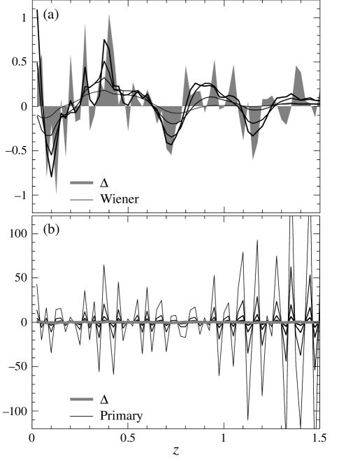
Figure 1: True radial density distribution (shaded) vs. (a) Wiener and (b) primary reconstructions, for a $4$ deg² pixel and source redshift bins with $\Delta z=0.025$ extending to $z_{\rm max}=2.5$. Thin lines correspond to the fiducial noise variance ($\bar{n}=3.6\times 10^{5}$ deg^-2 and $\gamma_{\rm rms}=0.3$), and lines of increasing thickness correspond to noise variance a factor of 10, 100, and 1000 times lower.

We show a sample realization in Fig. 1a (shaded) for a $\Lambda$CDM cosmology with with parameters $\Omega_{c}=0.3$, $\Omega_{b}=0.05$, $\Omega_{\Lambda}=0.65$, $h=0.65$, $n=1$, $\delta_{H}=4.2\times 10^{-5}$ ($\sigma_{8}=0.92$), pixel area of 4 deg² and redshift binning of $\Delta z=0.025$. We will use this as the fiducial cosmology in the examples that follow.

IV.3 Wiener Filter

As discussed in § II.1, Wiener filtering minimizes the reconstruction noise using prior knowledge of ${\bf S}_{{\Delta}{\Delta}}$, the covariance matrix of the signal. In Fig. 1, we compare the Wiener reconstruction with the primary map for a Gaussian realization of structure and several choices of the noise variance. The thinnest lines (smoothest for Wiener, noisiest for primary) correspond to the fiducial noise specifications ($\bar{n}=3.6\times 10^{5}$ deg^-2 and $\gamma_{\rm rms}=0.3$; see § II.3), and the noise variance decreases by factors of 10 as the lines thicken. Note the hundredfold difference in noise scale between the Wiener and primary reconstructions.

The primary reconstruction is far too noisy to recover a visual impression of the structure, even for wildly optimistic assumptions about the noise. However, the noise has a specific oscillatory structure arising from the noise covariance (see Eqn. (36)), which is neither completely random nor present in the true signal. The Wiener filter uses the information in the noise covariance of the primary reconstruction to reveal the hidden signal. For the fiducial noise specification, the Wiener filtered map recovers the low order, long-wavelength features in the density field; it is not until a prohibitively low noise variance is reached that fine-scale features of order the bin width are recovered.

The Wiener reconstruction is useful in cases where a map with well-defined statistical properties is needed, for example for cross-correlation studies with luminous tracers of the dark matter.

IV.4 KL Transform

In the low signal-to-noise regime, it is more quantitatively useful to express the data in terms of a new set of orthogonal basis functions that are rank ordered by their signal-to-noise ratio. Low signal-to-noise modes may be eliminated from the data set allowing a near lossless compression of the data. The pixel representation of these modes then tells us their correspondence to the radial density field. This is accomplished by the Karhunen-Loeve transform, also known as the signal-to-noise eigenmode technique (e.g. TegTayHea97 ).

Consider the generalized eigenmode problem,

$${\bf S}_{{\Delta}{\Delta}}{\bf e}={\epsilon}{\bf N}_{{\Delta}{\Delta}}{\bf e}\,.$$ (45)

With a Cholesky decomposition

$${\bf N}_{{\Delta}{\Delta}}={\bf L}_{\rm N}{\bf L}_{\rm N}^{t}\,,$$ (46)

the generalized eigenmode problem reduces to an ordinary one

$$\left[{\bf L}_{\rm N}^{-1}{\bf S}_{{\Delta}{\Delta}}{\bf L}_{\rm N}^{-t}\right][{\bf L}_{\rm N}^{t}{\bf e}]=\epsilon[{\bf L}_{\rm N}^{t}{\bf e}]\,.$$ (47)

The eigenvectors represent linear combination of the data ${\bf d}_{{\Delta}}$. If one composes the matrix with rows representing the eigenvectors

$${\bf R}_{{\rm K}{\Delta}}=\left(\begin{matrix}{\bf e}_{1}^{t}\\ ...\\ {\bf e}_{n_{z}}^{t}\end{matrix}\right)\,,$$ (48)

the new representation of the data vector becomes

$$\hat{\bf s}_{\rm K}={\bf R}_{{\rm K}{\Delta}}{\bf d}_{{\Delta}}\,.$$ (49)

The important property of the Karhunen-Loeve transform is that

$$\langle\hat{\bf s}_{{\rm K}}\hat{\bf s}_{{\rm K}}^{t}\rangle = {\bf R}_{{\rm K}{\Delta}}[{\bf S}_{{\Delta}{\Delta}}+{\bf N}_{{\Delta}{\Delta}}]{\bf R}_{{\rm K}{\Delta}}^{t}$$ (50)

$$\equiv {\bf S}_{{\rm K}{\rm K}}+{\bf N}_{{\rm K}{\rm K}}\,,$$

where the the covariance matrices satisfy the important condition

$${\bf S}_{{\rm K}{\rm K}} = \epsilon{\bf I}\,,$$

$${\bf N}_{{\rm K}{\rm K}} = {\bf I}\,,$$ (51)

such that the modes are uncorrelated separately in each. Furthermore, $\epsilon$ quantifies the relative contributions of signal and noise in the mode.

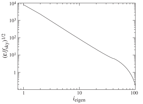
Figure 2: Signal-to-noise ratio in the Karhunen-Loeve eigenmodes with the sky-coverage scaled out, $(\epsilon/f_{\rm sky})^{1/2}$, calculated for $5^{\prime}\times 5^{\prime}$ pixels with the fiducial noise variance and redshift binning.

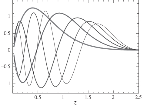
Figure 3: Signal-to-noise eigenmodes for the five largest eigenvalues in Fig. 2. The eigenmodes are similar to low frequency Fourier modes in the radial direction.

In Fig. 2, we show the signal-to-noise ratio per eigenmode $\epsilon^{1/2}$. This ratio is scaled by the square root of the fraction $f_{\rm sky}$ of the sky covered by a survey, to reflect the increase in the signal-to-noise for a statistical detection with independent pixels. Here we have assumed a pixel size of $5^{\prime}\times 5^{\prime}$, which is sufficiently small to extract most of the information on large-scale structure.

Note the steep decrease in the signal-to-noise ratio as a function of the eigenmode index: the first few eigenmodes contain most of the information. This fact allows a radical compression of the data, here from 100 bins to a handful. Nonetheless, even though the ratio is small for essentially all of the higher eigenmodes on the scale of individual pixels ($f_{\rm sky}\sim 2\times 10^{-7}$), a survey comprising 4–400 deg² ($f_{\rm sky}\sim 10^{-4}$–$10^{-2}$) has more than enough signal for a statistical detection.

To understand the information stored in the higher modes, we plot the first few eigenmodes in redshift in Fig. 3 renormalized to have unit norm. The first eigenvector simply shows the overall lensing efficiency when integrated over the whole source distribution, i.e. it has a single peak at a distance halfway to the median redshift $z=1$. The higher eigenvectors increase the number of nodes with the boundary conditions that the weight is negligible near the observer at $z=0$ and well beyond the median redshift. They are therefore the analogues of low order Fourier wavevectors in the radial direction.

These low order modes are sensitive to the cosmological model itself in that their values depend on the growth rate of structure, the volume element of the pixel-redshift bins, and the distances in the lensing efficiency. Even a statistical measure of their rms amplitude can help constrain cosmology, in particular the dark energy.

A potential problem for this use of three-dimensional mapping is that a cosmology is assumed both in the Karhunen-Loeve decomposition and in the projection matrix itself Eqn. (28). The former problem is readily handled in that even if the a priori assumption of the signal matrix in Eqn. (IV.1) is incorrect, the Karhunen-Loeve transform is a well-defined linear operation on the data. The modification comes about in the calculation of the covariance of the estimators in Eqn. (50). The covariance is still diagonal in the noise but need not be diagonal in the signal nor do its elements have the interpretation of signal-to-noise. Still, it is calculable for the purpose of model fitting and does not present a fundamental problem.

The second problem is apparently more subtle but reduces to the same issue. Errors in our cosmological assumptions in the projection matrix make the primary map not correspond precisely to a density reconstruction. Fortunately the form of the projection matrix is similar in all cosmologies: a broad bell-shaped weighting that peaks halfway to the source distance. Again, the well-defined linear operations involved allow us to predict the statistics of the primary map given a cosmology in spite of the fact that it does not strictly represent the density field.

Of course, if the recovered cosmology differs greatly from the assumed one, then the signal-to-noise eigenmodes will become an inefficient representation of the data. The best solution to both problems is to iterate the analysis and converge on a fiducial cosmology that fits the data.

V Individual Dark Matter Halos

Below $10^{\prime}$, the convergence field is dominated by individual structures, or dark matter halos, along the line-of-sight to the source galaxies. The abundance in redshift of such objects is well known to be exceedingly sensitive to the growth rate of structure and hence the dark energy in the universe abundance . Identification and mass measurement by lensing would be ideal because the association of luminous observables with the dark mass of the halos is always problematic. Indeed there may exist halos that are effectively dark darkcluster . However, the efficacy of a purely lensing-based study is severely compromised by projection effects projection , so three-dimensional mapping in principle holds the key to utilizing this fundamental test.

In the discrete halo case, one also has a well-motivated prior to regularize the inversion. In V.1, we discuss a modified version of the maximum entropy method. This method is most useful in the intermediate regime where the signal contains individual objects embedded in the large-scale structure. We then describe point source regularization, which is the best method when there is good reason to believe that effectively all of the structures are well localized and the large-scale structure component can be ignored.

V.1 Maximum Entropy Method

The maximum entropy method (MEM) is widely applied in situations where a noisy image is assumed to contain both discrete objects and a diffuse component (e.g. NarNit86 ) and has been applied to two-dimensional weak lensing data SeiSchBar98 . In this case the noisy image is the primary map ${\bf d}_{{\Delta}}$, the discrete objects are dark matter halos, and the diffuse component is the large-scale structure of the universe. MEM involves adding a penalty function to the mapmaking minimization of Eqn. (4) for the recovery of an MEM filtered signal ${\bf s}_{{\rm E}}$,

$$H=\lambda\sum_{i=1}^{n_{z}}I[{\bf s}_{{\rm E}}]_{i}\ln I[{\bf s}_{{\rm E}}]_{i}\,,$$ (52)

where the intensity $I$ is some functional of ${\bf s}_{\rm E}$ that we require to be positive. The Lagrange multiplier $\lambda$ trades off between minimizing $\chi^{2}$ and regularizing the solution. It is here chosen to give $\chi^{2}=\nu$, the degrees of freedom. The main feature of MEM is that while it prefers a uniform solution $I_{i}=$const., it does not additionally penalize bin-to-bin fluctuations as polynomial regularization would. Hence it allows solutions with discrete objects that occupy only one bin.

To apply MEM to our mass reconstruction we need to choose $I$. A natural choice would be $1+a_{i}[{\bf s}_{\rm E}]_{i}$ since the density cannot fluctuate to negative values. However this prescription would still strongly disfavor placing all of the mass in a single redshift bin. To allow us more freedom in the regularization let us take a more general form

$$I[x] = 1+x\,,$$

$$x = \delta_{\rm thr}\arctan\left(\frac{a_{i}[{\bf s}_{\rm E}]_{i}}{\delta_{\rm thr}}\right)\,.$$ (53)

The parameter $\delta_{\rm thr}$ places a threshold density above which MEM no longer penalizes the reconstruction; it returns the natural choice when $\delta_{\rm thr}\rightarrow\infty$.

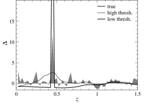
Figure 4: MEM reconstruction with a halo of $5\times 10^{14}h^{-1}M_{\odot}$ added to a $10^{\prime}\times 10^{\prime}$ pixel realization of large-scale structure (shaded) with the fiducial noise variance and redshift binning (see Fig. 1). High (thick line, $\delta_{\rm thr}=10$) and low (thin line, $\delta_{\rm thr}=3$) threshold cases are shown. The MEM solution makes a discrete transition between these stable solutions.

In Fig. 4 we show an example of the technique for the case of a halo embedded in large scale structure. For a high $\delta_{\rm thr}$ compared with the true density contrast of the halo, MEM seeks to regularize the reconstructed density in pixels and returns a smooth solution. For a $\delta_{\rm thr}$ that is lower, MEM places a density spike at the right position but the wrong amplitude. It favors a solution where the neighboring bins are all underdense since there is no penalty for further adding to the height of the spike.

A fundamental drawback of MEM is the difficulty in assessing the errors in the reconstruction, i.e. the reality of the discrete objects MEM finds. Note that by construction both solutions in Fig. 4 have exactly the same $\chi^{2}$, and the radical change in character of the solution is driven by the prior assumption of $\delta_{\rm thr}$ which sets the likelihood of having a comparable density spike in the solution. Still, MEM can identify interesting regions in the data for further study, perhaps with the point source method below. Conversely, it provides a useful cross check on the robustness of the point source solutions below.

V.2 Point Source Method

In regions that are known to be atypical of large-scale structure — either as flagged by the MEM reconstruction or simply because the signal in $\kappa$ is much too large to be generated by large-scale structure — it is reasonable to assume as a prior that the density field is dominated by a collection of discrete massive objects. Ironically, this form of anti-regularization of the density field in redshift bins is itself the most extreme regularization of the ones considered here, i.e. it has the least number of allowed degrees of freedom. The single-object form of this technique has been applied to data by Witetal01 and yields impressively precise predictions of the redshift or radial location. Whether the predictions are accurate, however, depends on the validity of the single-object assumption and on the regularization criteria more generally.

Let us state the criteria in a more general form. Define the penalty function on a point-source–regularized reconstruction ${\bf s}_{\rm H}$ as

$$H=\begin{cases}0&n_{\rm O}\leq n_{\rm H}\,,\\ \infty&n_{\rm O}>n_{\rm H}\,,\end{cases}$$ (54)

where $n_{\rm O}$ is the number of redshift bins occupied by a density fluctuation, and $n_{\rm H}$ is a prior assumption of the number of discrete objects (halos) the reconstruction should have. In other words, the minimization of Eqn. (4) is strictly over the position and density amplitude of $n_{\rm H}$ objects. The danger in this method of course is that it will return a best fit for the $n_{\rm H}$ objects even if the solution is in fact a smooth distribution or composed of some other number of objects.

A well-defined procedure that makes minimal use of prior information is to identify sky pixels like to contain one or more massive objects (as described above), and to perform a sequence of minimizations with $n_{\rm H}=1,2,\ldots$, stopping when the $\chi^{2}$ does not improve significantly.

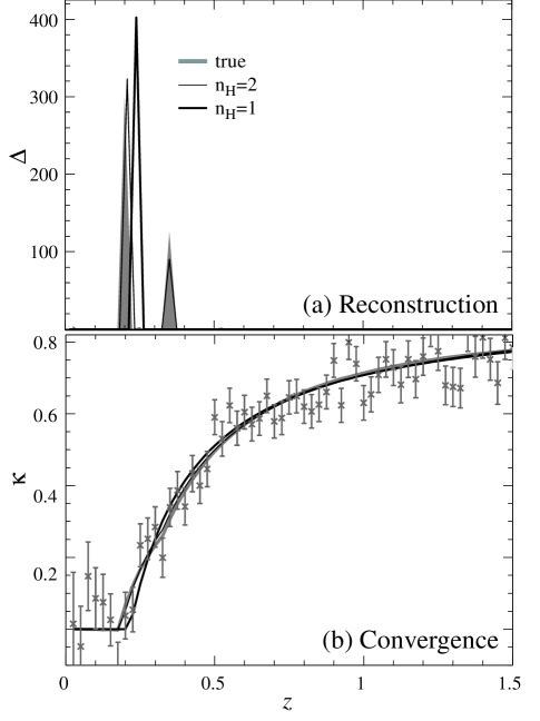
Figure 5: Point source method. (a) Density reconstruction for two halos of mass $10^{15}h^{-1}M_{\odot}$ each added to a $5^{\prime}\times 5^{\prime}$ pixel realization of large-scale structure (shaded), with the fiducial noise variance and binning (see Fig. 1). Priors of $n_{\rm H}=1$ (thin) and $n_{\rm H}=2$ halos (thick) are compared. (b) Original data in the convergence $\kappa$ compared with the reconstructions.

In Fig. 5a, we show an example with two very massive cluster-sized halos at $z=0.19$ and $z=0.34$. (The masses are enclosed entirely within the $5^{\prime}\times 5^{\prime}$ pixels and their respective redshift bins.) The fit assuming one point source returns $\chi^{2}=96$ for 100 redshift bins and two parameters — a perfectly good fit. The fit yields a redshift constraint $z=0.239\pm 0.006$ that is remarkably precise, but wrong. Going to $n_{\rm H}=2$ does recover two objects in the proper locations, with $\chi^{2}=91$ for two fewer degrees of freedom. In Fig. 5b we show the implied $\kappa$ fields plotted against the original data. The residuals for the one-object fit show coherent structure near the true halo locations and so the improvement in $\chi^{2}$ is significant. Still, this example warns against blindly interpreting the formal errors of the fit. It is actually an optimistic example because the large masses and redshift separation $(\Delta z=0.15)$ yield a signal much larger and much better separated than expected for real weak lensing measurements.

To better distinguish between close alternatives one could fold in prior information. For example, one could use the theoretically well-understood abundance of massive halos to determine the relative likelihood of the solutions given the recovered masses of the objects, e.g. two halos of $5\times 10^{15}$ $h^{-1}\,M_{\odot}$ may be favored over one halo of $10^{16}$ $h^{-1}\,M_{\odot}$ due to the predicted exponential suppression in the number density of high mass halos. One could also use model profiles to create matched filters across smaller pixels that resolve the halo. Finally, prior information from photometric redshifts of galaxies likely to be members of the cluster(s) could decide between competing solutions Witetal01 .

VI Discussion

We have shown that the evolution of the shear field in source redshift contains large-scale information about the distribution of dark matter, statistical information about its fluctuations on smaller scales, and redshift localization information for massive dark matter halos on the smallest scales where the signal is large. This information is hidden in the noise of a direct reconstruction, and its extraction requires mild prior assumptions about the statistical properties of the density field. We have argued for an approach that begins with a lossless direct or primary reconstruction that is followed by regularization by a prior that is appropriate for the information that is to be extracted.

In the large to intermediate scale regime, the information content can be distilled into signal-to-noise or KL eigenmodes which efficiently compress the data by a factor of 10 or more. These low-order modes probe the slow evolution of the statistics of the density field and are well suited to studying the properties of the dark energy. Tomographic sensitivity to the dark energy has been previously noted in the two-point correlation of the shear through the improvement of projected measures of the dark energy density and equation of state for future surveys tomopower . The KL eigenmode decomposition retains information from the higher order correlations in the field skewness and also establishes a more direct, non-parametric quantification of the information contained in the data. A full study of the cosmological implications is beyond the scope of this paper, but we believe that it will be a promising approach for the future.

Wiener filtering in the large-scale regime returns large scale maps of the density field with well-defined statistical properties. These should be useful in cross-correlation studies with luminous, biased tracers of the dark matter such as galaxies and galaxy clusters bias . With information on the radial dimension, information on the evolution of the bias can be recovered which in turn constrains the tracers’ formation and evolution.

In the individual halo regime, tomographic techniques have already been successfully applied to data Witetal01 . With a well-motivated prior on the number of discrete halos along the line of sight, the reconstruction can yield excellent localization of the object(s), in principle to a precision that is better than that in the source redshifts themselves. However the accuracy is compromised by an incorrect assumption of the number of objects. Here we advocate a combined approach of adding discrete objects to the fit, regularizing by maximum entropy, and employing prior information and followup.

While it is unfortunate that these prior assumptions are necessary for extracting information from three-dimensional reconstructions of the density field, they are generally well-motivated and testable. Gravitational lensing therefore remains our most direct, assumption-free means of probing the distribution of the dark matter.

Acknowledgments: We thank J. Frieman and A. Kravtsov for useful conversations. WH is supported by NASA NAG5-10840 and the DOE OJI program. CRK is supported by NASA through Hubble Fellowship grant HST-HF-01141.01-A from the Space Telescope Science Institute, which is operated by the Association of Universities for Research in Astronomy, Inc., under NASA contract NAS5-26555.

References

- (1)
- (2) D. Huterer, M.S. Turner, Phys. Rev. D, 64, 123527 (2001); L. Wang, R.R. Caldwell, J.P. Ostriker, P.J. Steinhardt, Astrophys. J, 530, 17 (2000).
- (3) J.A. Tyson, R.A. Wenk, F. Valdes, Astrophys. J, 349, 1 (1990).
- (4) R.D. Blandford, A.B. Saust, T.G. Brainerd, J.V. Villumsen, Mon. Not. Roy. Astr. Soc., 251, 600 (1991); J. Miralda-Escude, Astrophys. J, 380, 1 (1991); N. Kaiser, Astrophys. J, 388, 272 (1992).
- (5) D. Bacon, A. Refregier, R. Ellis, Mon. Not. Roy. Astr. Soc., 318, 625 (2000); N. Kaiser, G. Wilson, G.A. Luppino, Astrophys. J Lett., submitted, astro-ph/0003338 (2000); L. van Waerbeke, et al. Astron. Astrophys., 358, 30 (2000); D.M. Wittman, J.A. Tyson, D. Kirkman, I. Dell’Antonio, G. Bernstein, Nature, 405, 143 (2000).
- (6) D. Wittman, J.A. Tyson, V.E. Margoniner, J.G. Cohen, I.P. Dell’Antonio, Astrophys. J, 557, 89 (2001).
- (7) A.N. Taylor, Phys. Rev. Lett., submitted, astro-ph/0111605 (2001).
- (8) N. Kaiser, G. Squires, Astrophys. J, 404, 441 (1993).
- (9) M. Tegmark, Astrophys. J, 480, 87 (1997).
- (10) M. Bartelmann, P. Schneider, Phys. Rept., 340, 291 (2001); Y. Mellier, Ann. Rev. Astron. Astrophys., 37, 127 (1999).
- (11) P. Catelan, M. Kamionkowski, R.D. Blandford, Mon. Not. Roy. Astr. Soc., 323, 713 (2001); R. Crittenden, P. Natarajan, U. Pen, T. Theuns, Astrophys. J, 559, 552 (2001); R.A.C. Croft, C. Metzler, Astrophys. J, 545, 561 (2000); A.F. Heavens, A. Refregier, C. Heymans, Mon. Not. Roy. Astr. Soc., 319, 649 (2000).
- (12) A. de Oliveira-Costa, et al. Astrophys. J Lett., 509, L77 (1998); J.R. Bond, A.H. Jaffe, L. Knox, Phys. Rev. D, 58, 083004 (1998).
- (13) U. Seljak, Astrophys. J, 506, 64 (1998).
- (14) N. Kaiser, Astrophys. J, 498, 26 (1998).
- (15) B. Jain, U. Seljak, Astrophys. J, 484, 560 (1997).
- (16) J.A. Peacock, S.J. Dodds, Mon. Not. Roy. Astr. Soc., 280, 19 (1996).
- (17) M. White, W. Hu, Astrophys. J, 537, 1 (2000).
- (18) M. Tegmark, A.N. Taylor, A.F. Heavens, Astrophys. J, 480, 22 (1997); M.S. Vogeley, A.S. Szalay, Astrophys. J, 465, 34 (1996); J.R. Bond, Phys. Rev. Lett., 74, 4369 (1995); E.F. Bunn, N. Sugiyama, Astrophys. J, 446, 49 (1995).
- (19) N.A. Bahcall, X. Fan, Astrophys. J, 504, 1 (1998); A. Blanchard, J.G. Bartlett, Astron. Astrophys., 332, L49 (1998); P.T.P. Viana, A.R. Liddle, Mon. Not. Roy. Astr. Soc., 303, 535 (1999); Z. Haiman, J.J. Mohr, G.P. Holder, Astrophys. J, 553, 545 (2001).
- (20) T. Erben, et al. Astron. Astrophys., 355, 23 (2000); K. Umetsu, T. Futamase, Astrophys. J, 539, 5 (2000); J.M. Miralles, et al. Astron. Astrophys., submitted, astro-ph/0202122 (2002); N.N. Weinberg, M. Kamionkowski, Mon. Not. Roy. Astr. Soc., submitted, astro-ph/0203061 (2002).
- (21) M. White, L. van Waerbeke, J. Mackey, Astrophys. J, in press, astro-ph/0111490 (2001); K. Reblinsky, M. Bartelmann, Astron. Astrophys., 345, 1 (1999).
- (22) R. Narayan, R. Nityananda, Ann. Rev. Astron. Astrophys., 24, 127 (1986).
- (23) S. Seitz, P. Schneider, M. Bartelmann, Astron. Astrophys., 337, 325 (1998).
- (24) W. Hu, Astrophys. J Lett., 522, 21 (1999); D. Huterer, Astrophys. J, in press, astro-ph/0106399 (2002); W. Hu, Phys. Rev. D, 65, 023003 (2002).
- (25) F. Bernardeau, L. van Waerbeke, Y. Mellier, Astron. Astrophys., 322, 1 (1997); L. Hui, Astrophys. J, 519, 9 (1999).
- (26) P. Schneider, Astrophys. J, 498, 43 (1998); L.. van Waerbeke, Astron. Astrophys., 334, 1 (1998).