How large is our universe?

Abstract

We reexamine constraints on the spatial size of closed toroidal models with cold dark matter and the cosmological constant from cosmic microwave background. We carry out Bayesian analyses using the Cosmic Background Explorer (COBE) data properly taking into account the statistically anisotropic correlation, i.e., off-diagonal elements in the covariance. We find that the COBE constraint becomes more stringent in comparison with that using only the angular power spectrum, if the likelihood is marginalized over the orientation of the observer. For some limited choices of orientations, the fit to the COBE data is considerably better than that of the infinite counterpart. The best-fit matter normalization is increased because of large-angle suppression in the power and the global anisotropy of the temperature fluctuations. We also study several deformed closed toroidal models in which the fundamental cell is described by a rectangular box. In contrast to the cubic models, the large-angle power can be enhanced in comparison with the infinite counterparts if the cell is sufficiently squashed in a certain direction. It turns out that constraints on some slightly deformed models are less stringent. We comment on how these results affect our understanding of the global topology of our universe.

I INTRODUCTION

Is the universe finite or infinite? If we assume the “strong Copernican principle” (SCP) that the spatial hypersurface is globally and locally homogeneous and isotropic, then all three-spaces are classified by the sign of the curvature; spaces with a positive constant curvature are closed and finite in volume while spaces with a negative constant curvature or vanishing curvature are open and infinite. Hence, one might expect that the sign of the spatial curvature completely determines the size of our universe.

However, there is no particular theoretical reason for assuming the global homogeneity and isotropy of the spatial hypersurface, since the Einstein equation itself cannot specify the global topology of the space-time. In fact, there are a variety of cosmological models that satisfy the “weak Copernican principle” for which the spatial section is locally homogeneous and isotropic but not necessarily globally homogeneous and isotropic. These multiply connected (MC) models (for a comprehensive review see [1, 2, 3]) are topologically distinct but the metric is exactly the same as that of the simply connected counterparts with constant curvature. Therefore, these MC models are in harmony with the observational facts that support the Friedmann-Robertson-Walker (FRW) models, namely, the cosmic expansion, the relative amounts of primordial light elements, and the cosmic microwave background. In order to answer whether or not the spatial section of our universe is finite, we need to determine not only the curvature, but also the global spatial topology of the spatial hypersurface, since there are a number of closed compact spaces with a negative or a vanishing curvature.

If the spatial section is sufficiently small, then all the fluctuations beyond the comoving size of the space are suppressed. It has been claimed by several authors that the “small universes”[4] in which the topological identification scale is equivalent to or smaller than the horizon scale have been observationally ruled out because large-angle power of the cosmic microwave background (CMB) temperature fluctuations is significantly suppressed [5, 6, 7, 8] and does not fit to the Cosmic Microwave Background Explorer (COBE) Differential Microwave Radiometer (DMR) data.

However, for low matter density models $\Omega_{0}<1$, constraints on the size of the spatial section are less stringent, since the bulk of large-angle temperature fluctuations can be produced in the curvature or $\Lambda$ dominant era, leading to less stringent suppression in the large-angle power [9, 10, 11, 12].

On the other hand, it has been pointed out that constraining closed MC models using only the angular power spectrum is not sufficient, since it does not contain information about the anisotropic component of statistically averaged fluctuations [13]. In fact, temperature fluctuations in the sky for the MC models (except for the projective three-space $RP^{3}$) are described by an anisotropic Gaussian random field for a particular choice of position and orientation of the observer, provided that each Fourier mode is independent and obeys Gaussian statistics as predicted by the standard inflationary scenario. Therefore, in order to constrain the MC models, one must compare all anisotropic and inhomogeneous fluctuation patterns for every possible choice of orientation and position of the observer with the observed data, which needs time-consuming Monte Carlo simulations. Based on the study of several closed hyperbolic (CH) models, [13] claimed that all “small universes” are ruled out because the anisotropic correlation patterns are at variance with the COBE DMR data.

Nevertheless, for CH models, a subsequent analysis confirmed that the fit to the data depends not only on the orientation but also on the position of the observer. In some limited places, the likelihood is considerably higher than that of the simply connected counterpart[14]. Even if the place at which the pixel-pixel two-point correlation agrees with the data is limited, the model cannot be ruled out if the fit to the data is sufficiently good at certain places.

On the observational side, there has been mounting evidence that the spatial section of our universe is almost flat [15, 16, 17, 18]. If the background space is exactly flat, the topology of the orientable closed space is limited to six kinds [1]. The simplest space is the toroidal space $T^{3}$. Although closed flat MC models need a “fine-tuning” that the present horizon scale is comparable to the topological identification scale $L_{t},$ it is of crucial importance to give a lower bound on the size of the spatial section of these models, since we have no prior knowledge of the spatial topology of the universe.

In this paper, we improve the previous COBE bounds on the size of the spatial hypersurface of closed toroidal flat cold dark matter models with a consmological constant ($\Lambda$CDM) [19]by carrying out Bayesian analysis properly taking account of statistically anisotropic correlation that cannot be described by the angular power spectrum $C_{l}$. The temperature fluctuations are calculated by solving the linear evolution of the photon-baryon fluid from the COBE scale to the acoustic oscillation scale. We estimate the best-fit normalization of the power of the matter density fluctuations at the $8\textrm{h}^{-1}$Mpc scale $\sigma_{8}$ in comparison with those of simply connected $\Lambda$CDM models. Throughout this paper we assume that $\Omega_{m}\!=\!0.3,\Omega_{\Lambda}\!=\!0.7$. In Sec.II, we give a brief account of the temperature anisotropy on large to intermediate scales and we study how the size and the shape of the fundamental cell affect the large-angle anisotropy. In Sec.III, we carry out full Bayesian analyses using the COBE DMR data based on pixel-pixel correlation and obtain the likelihoods and the best-fit normalizations $\sigma_{8}$. In Sec.IV, we discuss the viability of other closed flat models, almost-flat closed spherical and almost-flat closed hyperbolic models. In Sec.V, we draw our conclusions and discuss the possibility of detecting the signature of the finiteness of the spatial geometry of the universe in the future.

II Temperature Anisotropy

In the Newtonian gauge, the $l$th multipole of the primary temperature anisotropy in the FRW models projected onto the sky at the conformal time $\eta$ is written in terms of the monopole $\Theta_{0}$, and the dipole $\Theta_{1}$ of temperature fluctuation and the Newtonian potential $\Psi$ at the last scattering and the time evolution of $\Psi$ and the Newtonian curvature $\Phi$[20],

$$\frac{\Theta_{l}(\eta,k)}{2l+1} = [\Theta_{0}+\Psi](\eta_{*},k)j_{l}(k(\chi(\eta)-\chi(\eta_{*})))+\Theta_{1}(\eta_{*},k)\frac{1}{k}\frac{d}{d\eta}j_{l}(k(\chi(\eta)-\chi(\eta_{*})))$$ (1)

$$+ \int_{\eta_{*}}^{\eta}\Bigl{(}\frac{\partial\Psi}{\partial\eta^{\prime}}-\frac{\partial\Phi}{\partial\eta^{\prime}}\Bigr{)}j_{l}(k(\chi(\eta)-\chi(\eta^{\prime})))d\eta^{\prime},$$ (2)

where $k$ denotes the wave number, $\eta_{*}$ is the last scattering conformal time, the radial distance is $\chi(\eta)=\eta$ and $j_{l}$ represents the $l$th-order spherical Bessel function. The first term in the right-hand side in equation (2) represents the “ordinary” Sachs-Wolfe (OSW) effect caused by the fluctuations in the gravitational potential at the last scattering. The second term describes the Doppler shift owing to the bulk velocity of the photon-baryon fluid. Note that this term is negligible at superhorizon scales $k\!\eta\!<1$ since radiation pressure cannot play any role and cosmic expansion damps away the initial velocity. The third term represents the integrated Sachs-Wolfe (ISW) effect caused by the decay of the gravitational potential.

In order to constrain the FRW models that yield isotropic Gaussian fluctuations, one needs only two-point correlations of temperature fluctuations $\Delta T/T$ in the sky, which can be characterized by the angular power spectrum $C_{l}=\langle|a_{lm}|^{2}\rangle$,

$$\frac{2l+1}{4\pi}C_{l}\propto\frac{1}{2\pi^{2}}\int_{0}^{\infty}{dk\over k}k^{3}\frac{|\Theta_{l}(\eta_{0},k)|^{2}}{2l+1},$$ (3)

where $a_{lm}$ represents the expansion coefficient with respect to the spherical harmonic $Y_{lm}$, $\langle\rangle$ denotes an ensemble average over the initial fluctuations, and $\eta_{0}$ is the present conformal time. Note that $C_{l}$ is invariant under any $SO(3)$ transformations.

Now, let us consider a closed toroidal model $T^{3}$ in which the spatial hypersurface is described by a cube with side $L$ in the Euclidean three-space whose opposite faces are identified by translations. Then the wave numbers of the square-integrable eigenmodes of the Laplace-Beltrami operator are restricted to the discrete values $k_{i}=2\pi n_{i}/L$, ($i=1,2,3$) where $n_{i}$’s run over all integers. Equation $(\ref{eq:cl})$ now reads

$$\frac{2l+1}{4\pi}C_{l}\propto\frac{1}{L^{3}}\sum_{{\mathbf{k}}\neq 0}\frac{|\Theta_{l}(\eta_{0},k)|^{2}}{2l+1}.$$ (4)

Note that all the modes whose wavelength is longer than $L$ are not where $a_{lm}$ represents the expansioallowed (“mode cutoff”). From now on, we restrict ourselves to the adiabatic scale-invariant Harrison-Zel’dovich spectrum $n\!=\!1$ [i.e., ${\cal{P}}_{\Phi}(k)\!=\!k^{3}\langle|\Phi(0,k)|^{2}\rangle\!=\!const.$] as predicted by the standard inflationary scenario. Note that $\Delta T_{l}=[l(l+1)C_{l}/(2\pi)]^{1/2}$ becomes almost flat for the Einstein-de Sitter universe. For low-density FRW models, the large-angle power is boosted owing to the ISW effect, since $\Lambda$ dominant epochs come earlier. However, for $T^{3}$ models, the OSW contribution to the large-angle power is suppressed because all modes whose wavelength is longer than the cutoff scale $L$ are not allowed. The angular scale below which the power is suppressed is approximately given by $l_{cut}=2\pi\eta_{0}/L-1$ [19]. Interestingly, for low-density $T^{3}$ models with moderate size of the cell, the excess power owing to the ISW contribution is almost canceled out by the suppression owing to the mode cutoff. As shown in figure (1), the suppression in the large-angle power is not prominent even for a model with $\epsilon\equiv L/2\eta_{0}=0.2$.

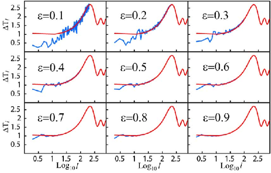
FIG. 1.: Plots of the angular power spectrum $\Delta T_{l}=[l(l+1)C_{l}/(2\pi)]^{1/2}$ for cubic toroidal models with various linear sizes parametrized by the ratio of the length of the side to the diameter of the last scattering surface in the comoving coordinates:$\epsilon=L/2\eta_{0}$ in comparison with that for the simply connected counterpart (solid curve). $\Delta T_{l}$ is normalized by $\Delta T_{10}$ for the simply connected models. Cosmological parameters are $\Omega_{\Lambda}=0.7$, $\Omega_{CDM}=0.26$, $\Omega_{b}=0.04$, and $h=0.7$.

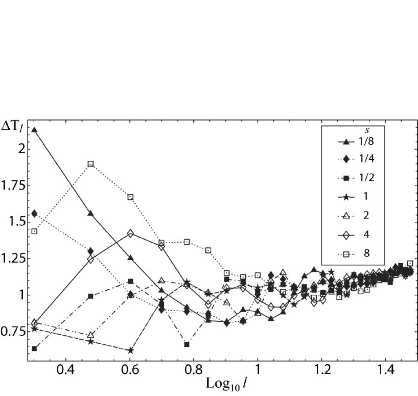
FIG. 2.: Plots of the angular power spectrum $\Delta T_{l}=[(l+1)C_{l}/(2\pi)]^{1/2}$ for deformed toroidal models whose fundamental cell is described by a rectangular box with sides $L_{1}\!=\!L_{2},L_{3}$. The volume is fixed to $V=(0.4\times 2\eta_{0})^{3}$. The degree of deformation is parametrized by $s\equiv(L_{1}=L_{2})/L_{3}$. $\Delta T_{l}$ is normalized by $\Delta T_{10}$ for the simply connected counterpart. In the small-angle limit $l\gg 1$, the angular power spectrum converges to that of the simply connected counterpart. Cosmological parameters are the same as in figure 1.

Next, we consider models in which the fundamental cell is described by a rectangular box $D$ with length $L_{i}$ of sides. We call these models the “pancake’ type or the “cigar” type if $D$ has a relatively long side in one direction, or long sides in two orthogonal directions, respectively. As shown in figure 2, the large-angle power is enhanced for models with a sufficiently squashed cell. It seems that the enhancement is rather surprising since Fourier modes whose wavelength is larger than the size of the cell are not allowed. The apparent enhancement is related to the number density of the Fourier modes. In order to see this, let us consider the number function defined as the number of eigenmodes of the Laplace-Beltrami operator whose eigenvalue is less than $E=k^{2}$, which is described by Weyl’s formula in the small-scale limit $N(E)=Vk^{3}/2\pi^{2}$, where $V$ denotes the volume of the three-space. For globally “almost” isotropic spaces like cubic toroidal spaces, the Weyl’s formula gives a good approximation of $N(k)$ in the large-scale limit as well. However, for globally “very” anisotropic spaces , the deviation from the Weyl formula is prominent in the large scale limit. For instance, the number function is approximately given by $N\propto k$ for the “cigar” type and $N\propto k^{2}$ for the “pancake” type [21]. The discrete wave number is given by

$$k=2\pi\sqrt{\frac{n_{1}^{2}}{L_{1}^{2}}+\frac{n_{2}^{2}}{L_{2}^{2}}+\frac{n_{3}^{2}}{L_{3}^{2}}},$$ (5)

where each $n_{i}$ runs over all integers. Hence, for $L_{2},L_{3}\ll L_{1}$, the modes on large scales $k\ll 1/L_{2},1/L_{3}$ are given by $k=2\pi n_{1}/L_{1}$, leading to $N(k)\sim L_{1}k/\pi$. Similarly, if $L_{3}\ll L_{1}\sim L_{2}$, the modes on large scales $k\ll L_{3}$ are given by $k=2\pi\sqrt{\frac{n_{1}^{2}}{L_{1}^{2}}+\frac{n_{2}^{2}}{L_{2}^{2}}}$, then $N(k)\sim L_{1}L_{2}k^{2}/4\pi$. Because the power is normalized by the total volume, the contribution of modes on large scales are relatively boosted, resulting in an enhancement in the large-angle power. Interestingly, for slightly squashed models, the reduction in the large-angle power owing to the mode cutoff is almost canceled out by the enhancement owing to the squeezing of the space.

Although we have assumed that the primordial power spectrum is scale-invariant even in the case of deformed models, the non-trivial boundary condition on the mode functions of inflaton fields may cause a deviation from the scale-invariant spectrum. However, such a deviation is expected to be small, since the background space time has a high degree of symmetry locally at the inflationary epoch that is relevant to the $n=1$ spectrum.

So far, we have studied the effect of the nontrivial global topology on the large-angle power. However, the angular power spectrum is not sufficient for constraining the models since the temperature fluctuations in the MC models are not statistically isotropic in general; the effect of off-diagonal elements $\langle a_{lm}a^{*}_{l^{\prime}m^{\prime}}\rangle$ for $l\neq l^{\prime}$ or $m\neq m^{\prime}$ which are not SO$(3)$ invariants cannot be negligible. Therefore, it is necessary to perform Bayesian analyses taking account of these off-diagonal elements for each possible orientation of the observer, since the toroidal models are globally anisotropic.

III Bayesian analysis

Any Gaussian temperature fluctuations in the sky can be characterized by a covariance matrix whose elements at pixel $i$ and pixel $j$ are,

$$M_{ij}=\langle T_{i}T_{j}\rangle=\sum_{ll^{\prime}mm^{\prime}}\langle a_{lm}a^{*}_{l^{\prime}m^{\prime}}\rangle W_{l}W_{l^{\prime}}Y_{lm}(\hat{\textbf{n}}_{i})Y_{l^{\prime}m^{\prime}}(\hat{\textbf{n}}_{j})+\langle N_{i}N_{j}\rangle$$ (6)

where $a_{lm}$ is an expansion coefficient with respect to a spherical harmonic $Y_{lm}$, and $\langle\rangle$ denotes an ensemble average taken over all initial fluctuations for a fixed orientation of the observer. $T_{i}$ represents the temperature at pixel $i$, $W_{l}^{2}$ is the experimental window function that includes the effect of beam smoothing and finite pixel size, $\hat{\textbf{n}}_{i}$ denotes the unit vector toward the center of pixel $i$, and $\langle N_{i}N_{j}\rangle$ represents the noise covariance between pixel $i$ and pixel $j$.

If we assume a uniform prior distribution for the cosmological parameters, from Bayes’ theorem, the probability distribution function of a set of $C^{l^{\prime}m^{\prime}}_{lm}\equiv\langle a_{lm}a^{*}_{l^{\prime}m^{\prime}}\rangle$ for a random Gaussian field (not necessarily isotropic) is given by

$$\Lambda(C^{l^{\prime}m^{\prime}}_{lm}|\vec{T})\propto\frac{1}{\det^{1/2}M(C^{l^{\prime}m^{\prime}}_{lm})}\exp\Biggl{(}\frac{1}{2}\vec{T}^{T}\cdot M^{-1}(C^{l^{\prime}m^{\prime}}_{lm})\cdot\vec{T}\Biggr{)}.$$ (7)

In the following analysis, we use the inverse-noise-variance-weighted average map of the 53A, 53B, 90A, and 90B COBE DMR channels. To remove the emission from the galactic plane, we use the extended galactic cut (in galactic coordinates) [22]. After the galactic cut, the best-fit monopole and dipole are removed using the least-squares method. To achieve efficient analysis in computation, we compress the data at “resolution 6” $(2.6^{o})^{2}$ ($l\sim 72$) pixels into one at “resolution 4” $(10.4^{o})^{2}$ ($l\sim 18$) pixels for which there are 384 pixels in the celestial sphere and 248 pixels surviving the extended galactic cut. The window function is given by $W_{l}=G_{l}F_{l}$ where $F_{l}$ are the Legendre coefficients for the DMR beam pattern [23] and $G_{l}$ are the Legendre coefficients for a circular top-hat function with area equal to the pixel area, which account for the pixel smoothing effect [24]. We also assume that the noise in the pixels is uncorrelated from pixel to pixel, which is known to be a good approximation[25].

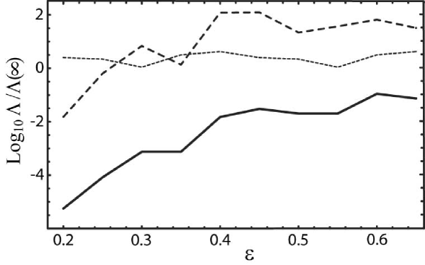
FIG. 3.: COBE constraints on cubic models. The solid curve represents the likelihoods $\Lambda$ marginalized over 24000 orientations of the observer and the normalization for various relative linear size $\epsilon=L/2\eta_{0}$. The dashed line shows the maximum values. The dotted line represents the likelihoods computed by neglecting the anisotropic components. All the likelihoods are normalized by that of the simply connected counterpart $\Lambda(\infty)$. Cosmological parameters are the same as in figure 1.

Because the toroidal $T^{3}$ model is globally anisotropic, the two-point pixel-pixel correlations depend on the orientation of the coordinate axes. Therefore, we need to compute the likelihood function for each orientation $\alpha$ of the observer. Assuming a constant distribution for $\alpha$ and the normalization $\sigma$, the likelihood is given by $\Lambda=\int\Lambda(\alpha,\sigma)d\alpha d\sigma$, where $d\alpha$ denotes the volume element of a Lie group SO$(3)$ with Haar measure.

As shown in figure 3, the angular power spectrum alone does not give a stringent constraint $\epsilon>0.3$ on the size of the cell. However, if we use a likelihood function taking account of anisotropic two-point correlations marginalized over the orientation of the observer, we obtain a rather stringent constraint.

Because there is no upper limit for $\epsilon$, we choose a variable $N=\pi/6\epsilon^{3}=$(volume of the observable region at present)/(volume of space at present) as a physical quantity that is assumed to be constantly distributed. We find that the logarithm of relative likelihoods $\log_{10}[\Lambda(N)/\Lambda(N=0)]$ for cubic models ($0.2\leq\epsilon\leq 0.65$) can be well fitted by a polynomial function $-bN^{a}$ where $a\!=\!0.46,b\!=\!0.78$ which are obtained by minimizing $\chi^{2}$. By marginalizing over $N$, we find a constraint $N\!\lesssim\!2.4$ ($\epsilon\!>\!0.6$) at 68% CL, and $N\!\lesssim\!8.2$ ($\epsilon\!>\!0.4$) at 95% CL corresponding to $\log_{10}\Lambda/\Lambda(\infty)\sim-0.9$, $\log_{10}\Lambda/\Lambda(\infty)\sim-2.0$, respectively. The constraint on the size of the spatial section is more stringent compared with the previous analysis [19] in which fluctuations on smaller angular scales $l\!\geq\!10$ have not been taken into account.

It should be emphasized that the likelihoods depend sensitively on the orientation of the observer, especially for models with small sides $\epsilon\ll 1$. The maximum value of the likelihood far exceeds the mean by a factor $\Lambda_{\max}/\Lambda=10^{2.5-3.9}$ for $0.2\leq\epsilon\leq 0.7$ which suggests that almost all the orientations are ruled out. For instance, $\Lambda_{\max}/\Lambda\sim 10^{3.9}$ implies that the likelihood attains high values only when the axes are oriented with a precision of $\sim 5^{o}$ which is equal to one half the size of one pixel.

To see the orientations that give the enormous likelihood, we have plotted the orientations in the skymap that give a large likelihood. Except for $\epsilon=0.2$, in which a weak correlation to the galactic pole is found, no particular preferred orientation is found (figure 4).

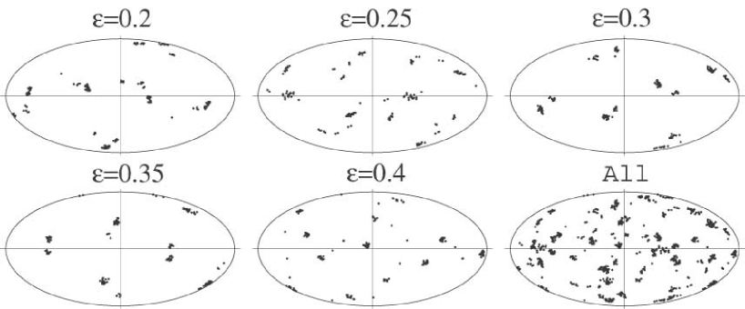
FIG. 4.: Best-fit orientations in the skymap for five cubic models. Each orientation is described by a set of six points that correspond to directions to the centers of the face of the cube that are preserved by the symmetries of $T^{3}$. A total of 40 orientations that give more than 80 percent contribution to the averaged likelihoods are plotted for each model. All the orientations for the five models are shown together in the last figure. The Aitoff projection is used. The center of the oval represents the galactic center.

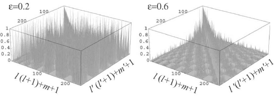
FIG. 5.: The contribution of off-diagonal elements for cubic models. The plotted lines represent $|\langle a_{lm}a^{*}_{l^{\prime}m^{\prime}}\rangle|/\sqrt{\langle a_{lm}a^{*}_{l^{\prime}m^{\prime}}\rangle\langle a_{lm}a^{*}_{l^{\prime}m^{\prime}}\rangle}$ for $2\!\leq\!l\!\leq\!15$, in ascending order of $l(l+1)+m+1$ and $l^{\prime}(l^{\prime}+1)+m^{\prime}+1$ for two types of cubic models.

In the previous literature, the effect of the global anisotropy has been considered to be small for cubic cases, because the contribution of off-diagonal elements is quite small. This argument is valid as long as one considers the averaged values over all the possible set of parameters $(l,l^{\prime},m,m^{\prime})$. Let us consider a set of orthogonal coordinates $(x,y,z)$ in which all the faces of the cube are perpendicular to one of the coordinate axes. Because of the symmetries of $T^{3}$, $\langle a_{l,m}a^{*}_{l^{\prime},m^{\prime}}\rangle$ vanishes if $l+l^{\prime}$ is even and $(m+m^{\prime})/2$ is even. In fact, the contribution of off-diagonal elements relative to the diagonal elements are small as 0.042 to 0.015 for $\epsilon\!=\!$0.2 to 0.6 for an ensemble of all values of $(l,l^{\prime},m,m^{\prime})$. However, as shown in figure 5, each nonzero component of off-diagonal elements is not so small (0.33 to 0.12 for $\epsilon\!=\!$ 0.2 to 0.6). Although any rotation of the coordinates gives a different structure in the off-diagonal components, the spiky structure cannot be completely vanished by any rotation.

One might argue that computing a likelihood marginalized over every orientation is meaningless and the constraint should be given by the maximum value of the likelihood instead of the marginalized value. Then the constraint becomes less stringent $\epsilon>0.25$. However, if we assume that the universe does not prefer a specific orientation, the cases of the “failed orientations” should be taken into account. By deforming the shape of the fundamental cell, or by changing the amplitude of the fluctuations, there might be a chance that the fluctuation fits the data almost perfectly, since the data themselves are anisotropic. In order to check this, a similar analysis has been carried out for deformed toroidal models whose fundamental cell is described by a rectangular box with sides $L_{1}=L_{2}$ and $L_{3}$. As shown in figure 6, the “pancake” type models $(L_{1}=L_{2})/L_{3}>1$ give much better fits to the data. For instance, for $s=10^{1/2}$, the likelihood is improved by 10 times in comparison with the cubic model with the same volume $V=(0.4\times 2\eta_{0})^{3}$. The corresponding number of copies of the fundamental cell inside the last scattering surface in the comoving coordinates is $N\!=\!8$ and the minimum linear size of the cell is equal to $L_{3}/2\eta_{0}=0.19$.

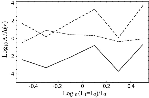
FIG. 6.: COBE constraints on deformed models whose fundamental cell is described by a rectangular box with sides $L_{1}\!=\!L_{2}$ and $L_{3}$. The volume is fixed to $V=(0.4\times 2\eta_{0})^{3}$. The solid curve represents the likelihoods $\Lambda$ marginalized over 24000 orientations of the observer and the normalization for various models. The dashed line shows the maximum values. The dotted line represents the likelihoods computed by neglecting the anisotropic components. All the likelihoods are normalized by that of the simply connected counterpart $\Lambda(\infty)$. Cosmological parameters are the same as in figure 1.

In the previous literature, it has also been argued that an increase in the best-fit normalization constant is related to the large-angle suppression owing to the finite size of the spatial section [12]. From our analyses, it is found that inclusion of off-diagonal term can also give a comparable increase in the best-fit normalization constant as well. For instance, the best-fit normalization $\sigma_{8}$ is increased by $\sim 10$ percent for $\epsilon=0.6$ (figure 7). The effect is relevant to the globally anisotropic geometry of the background space (see the appendix) which has been found for closed hyperbolic models (although the effect of the global inhomogeneity is neglected) [13].

If the best-fit normalization is too large, the choice of orientation is less probable (figure 8) (see the appendix). We have checked that the anticorrelation between the likelihood and the best-fit normalization becomes weaker and the plotted points get more aligned as the comoving size of the spatial section increases.

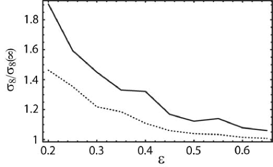
FIG. 7.: Plots of the ratio of the best-fit normalization of the cubic models to that of the simply connected counterpart (solid curve) and those obtained by an analysis in which the covariance matrix is computed by neglecting the off-diagonal terms (dotted curve).

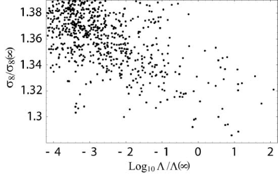
FIG. 8.: Plots of the best-fit normalization versus the likelihood for various orientations of the observer. The size of a cubic cell is $\epsilon=0.4$. Each quantity is normalized by the value for the simply connected counterpart.

IV Other Topologies

In addition to the toroidal models $T^{3}$ we have considered, there are five other flat orientable topologies, which can be realized as compact quotients of $T^{3}$, namely, $T^{3}/\textbf{Z}_{2},T^{3}/\textbf{Z}_{4},T^{3}/\textbf{Z}_{2}\times\textbf{Z}_{2},T^{3}/\textbf{Z}_{3}$, and $T^{3}/\textbf{Z}_{6}$ where $\textbf{Z}_{m}$ is a cyclic group of order $m$. The eigenmodes of the Laplace-Beltrami $\Delta$ operator can be written in terms of a finite sum of eigenmodes (= plane waves) of $T^{3}$,

$$u_{\textbf{k}}(\textbf{x})\propto\sum_{g_{i}\in\Gamma}\exp[i\textbf{k}\cdot(g_{i}\textbf{x})],$$ (8)

where $\Gamma$ denotes the discrete isometry group of $T^{3}$ and x is the Euclidean coordinates. Let us consider the case of $T^{3}/\textbf{Z}_{2}$, which can be realized by identifying the two pairs of opposite faces of a cube with sides $L$ by translations but for one pair of faces with a translation with $\pi$ rotation. Because the finite-sheeted covering space is described by a rectangular box with sides $L,L,2L$, one might expect that the space can support a mode with wavelength 2$L$. However, this is not true[26]. In fact, equation (8) yields the explicit form of the eigenmodes

$$u_{\textbf{k}}(\textbf{x})\propto\exp[i\textbf{k}\cdot\textbf{x}]+\exp[-i(k_{1}x_{1}+k_{2}x_{2}+ik_{3}(x_{3}+L)],$$ (9)

where $k_{1}=2\pi n_{1}/L,k_{2}=2\pi n_{2}/L,k_{3}=\pi n_{3}/L$. A mode with $n_{1}=n_{2}=0,n_{3}=1$ is equal to zero. Thus the allowed minimum wave number is still $k=2\pi/L$. Similarly, one can show that the maximum wavelength of the eigenmodes is comparable to the topological identification scale $L_{t}$ for other four cases[26]. Therefore, it is reasonable to conclude that the constraints on these closed flat models do not grossly differ from those on $T^{3}$ models.

Although we have assumed that the background space is exactly flat so far, it should be emphasized that a slight deviation from the flat space means a significant difference in the global topology. For instance, if the background space is exactly flat, there is no particular scale that sets the limit on the comoving size of the topological identification scale $L_{t}$. In other words, one can consider arbitrarily small or large spaces. However, for positively curved (spherical) or negatively curved (hyperbolic) spaces, the curvature radius $R_{c}$ sets a certain limit on the size of the space.

For instance, it has been proved that closed hyperbolic spaces with volume larger than $0.16668\cdots R_{c}^{3}$ cannot exist[27]. The smallest known CH space has volume $V=0.94R_{c}^{3}$[28]. Remembering that the volume of a ball with radius $R$ (proper length) in hyperbolic space is given by $V=\pi R_{c}^{3}[\sinh(2R/R_{c})-2R/R_{c}]$, the topological identification scale of CH spaces with $V\sim R_{c}^{3}$ is estimated as $L_{t}\sim R_{c}$. In this case, $\Omega_{K}^{-1/2}=R_{c}/H^{-1}\sim L_{t}/H^{-1}$ which gives $L_{t}\sim H^{-1}$ for $\Omega_{K}=0.1$ and $L_{t}\sim 10H^{-1}$ for $\Omega_{K}=0.01$. Thus, the effect of the global topology is almost negligible if $\Omega_{K}\ll 0.1$. However, if the spatial geometry is squashed in a certain direction while keeping the volume finite, the imprint of the global topology could be still prominent as in the case of flat topology although the enhancement in the large-angle power may put a limit on the possible shape of the fundamental cell. Moreover, if we allow CH orbifold models with a set of fixed points, then the volume can be as small as $V=0.0391R_{c}^{3}$[14]. Then the effect of the nontrivial global topology is conspicuous even if the space is as nearly flat as $\Omega_{K}=0.05$[14, 29].

In the case of spherical topology, the volume is written in terms of the order $|\Gamma|$ of the discrete isometry group $\Gamma$ of SO$(4)$, $V=2\pi^{2}R_{c}^{3}/|\Gamma|$[1]. Thus, the largest space is the three-sphere $S^{3}$ itself. On the other hand, there is no lower bound for the volume since one can consider a group with arbitrarily large number of elements of $\Gamma$. For instance, one can consider a cyclic group $\textbf{Z}_{m}$ with arbitrarily large $m$. Then $V=2\pi^{2}R_{c}^{3}/|\textbf{Z}_{m}|$ can be arbitrarily small and the obtained quotient space is squashed in one direction. As in CH models, the imprint of the global topology can be prominent for squashed spaces, even if the space is as nearly flat as $\Omega_{K}=0.05$ [30].

V Conclusion

In this paper, constraints on closed toroidal models from the COBE data have been reconsidered. By performing Bayesian analyses taking into account anisotropic correlation (i.e., off-diagonal elements in the covariance matrix) that has been often igonored in the previous literature, we obtained a constraint on the linear size of a cubic cell $L\gtrsim 0.6\times 2\eta_{0}$ for $\Omega_{\Lambda}\!=\!0.7,\Omega_{m}\!=\!0.3$ based on the likelihoods that are marginalized over the orientation of the observer. The maximum allowed number $N$ of copies of the cell inside the last scattering surface is $\!\sim\!2.4$ (68% CL). We find that the constraint becomes more stringent in comparison with that using only the angular power spectrum. The best-fit normalization $\sigma_{8}$ can be increased by $\sim$ 10 percent owing to the suppression in the large-angle power and the globally anisotropic geometry. We find that the likelihood depends sensitively on the orientation of the observer. Even if the likelihood that is marginalized over the orientation is small, the fit to the data for some limited set of orientations is far better than that of the infinite counterpart [14]. If one takes the maximum likelihood value instead, the constraint becomes conspicuously less stringent. Moreover, for some slightly deformed toroidal models, we find that the large-angle power can be flat and the constraint also becomes less stringent $N\sim 8$ (see also [31]).

In order to detect the periodic structure owing to the nontrivial topology, the topological identification scale (more precisely twice the injectivity radius at the observing point) must be smaller than the diameter of the last scattering surface in comoving coordinates: $L_{t}/2\eta_{0}<1$. Therefore, the present constraints do not completely deny the possibility of detection of periodic structure by future observations[32].

Even in the case of $L_{t}/2\eta_{0}\sim 1$, the signature of nontrivial topology might be observable as a nontrivial correlation structure in the temperature correlations [33] because the fluctuations in the MC models are non-Gaussian for isotropic and homogeneous observers. Inhomogeneous and anisotropic Gaussian fluctuations for a particular choice of position and orientation are regarded as non-Gaussian fluctuations for a homogeneous and isotropic ensemble of observers[34, 35]. If non-Gaussian fluctuations with vanishing skewness but non-vanishing kurtosis are found only on large angular scales in the CMB, then it will be a strong sign of the nontrivial topology, or equivalently the breaking of the SCP [2, 36, 37, 38]. Even if we failed to detect the identical patterns or objects in the sky, the imprint of “finiteness” could be still observable by measuring such statistical quantities. As we have discussed, the MC spaces can be squeezed irrespective of the type of topology. Even if the volume of the spatial section is large, we might be able to detect globally anisotropic structure if the spatial section is sufficiently squeezed in a certain direction, The ongoing satellite missions such as MAP and Planck will provide us an answer to the question “how large is our universe?”.

VI acknowledgments

We would like to thank K. Tomita for his continuous encouragement. The numerical computation was carried out on an SGI origin 3000 at Yukawa Institute Computer Facility. K.T.I. is supported by JSPS Research Fellowships for Young Scientists. This work was supported partially by Grant-in-Aid for Scientific Research Fund (No.14540290, No.11367).

A Anisotropic Gaussian Fluctuations

For homogeneous and isotropic Gaussian fluctuations, the variance of the expansion coefficient $a_{lm}$ is constant in $m$ for a given $l$ regardless of the position and orientation of the observer. In other words, there is no “$m$-structure” or “direction-direction” correlation in the expansion coefficients. On the other hand, for anisotropic Gaussian fluctuations, the variance of $a_{lm}$ depends on $m$ [34]. Because $a_{lm}$’s extracted from the data actually depend on $m$ owing to the cosmic variance, for some very limited choices of the orientation, the “$m$-structure” in the anisotropic fluctuations may agree with the apparent “$m$-structure’ in the data.

To confirm this, we compare the variances of expansion coefficients $b_{lm}$ of the best-fit case to those extracted from the data, which can be obtained by multiplying the temperature fluctuation $T_{i}$ and the standard deviation in the noise $N(\Omega_{i})$ by spherical harmonics $Y_{lm}$, and carrying out an integration over the pixels surviving the “extended” galactic cut (denoted as $S\!K$)

$$b_{lm}\equiv\sum_{l^{\prime}m^{\prime}}a_{l^{\prime}m^{\prime}}W_{l^{\prime}}\int_{S\!K}Y_{l^{\prime}m^{\prime}}(\Omega)Y^{*}_{lm}(\Omega)d\Omega+\int_{S\!K}N(\Omega)Y^{*}_{lm}(\Omega)d\Omega.$$ (A1)

As shown in figure 7, an excellent agreement at $l=6-7$ is observed. Because the theoretical prediction of the quadrapole is somewhat higher than the observed value, the large-angle suppression owing to the finite size of the spatial section is not relevant. We also checked other cases that give a large value in the likelihood compared to that of the simply connected counterpart and again such an excellent agreement in $|b_{lm}|$ at certain range of angular scales is observed for each case. Thus, for a limited choice of orientation, globally anisotropic Gaussian fluctuations can give a better fit compared with globally isotropic and homogeneous Gaussian fluctuations.

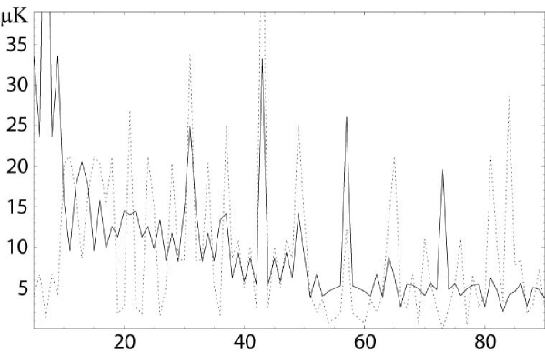
FIG. 9.: Plots of $|b_{lm}|=\sqrt{\langle b_{lm}b^{*}_{lm}\rangle}$ in ascending order of $l(l+1)+m+4$ for the $T^{3}$ cubic model (solid curve) with $\epsilon=0.4$ (solid curve) which best fits $b_{lm}$ extracted from the COBE DMR data (dashed curve).

Next, we consider the effect of off-diagonal elements in the two-point correlation $\langle a_{lm}a^{*}_{l^{\prime}m^{\prime}}\rangle$, $l\neq l^{\prime}$ or $m\neq m^{\prime}$, which represent scale-scale correlations.

For illustrative purpose, first, we consider a toy model in which the fluctuations obey a bivariate Gaussian distribution function,

$$p(y_{1},y_{2},\sigma,\tau)=\frac{1}{2\pi\sigma^{2}\sqrt{1-\tau^{2}}}\exp\Biggl{[}-\frac{1}{2(1-\tau^{2})}\Biggr{(}\frac{y^{2}_{1}+y^{2}_{2}-2\tau y_{1}y_{2}}{\sigma^{2}}\Biggr{)}\Biggr{]},$$ (A2)

where $\tau=\textrm{cov}(y_{1},y_{2})/\sigma^{2}$ is the correlation coefficient which represents the off-diagonal components. By an orthogonal transformation, $y_{1}=(x_{1}+x_{2})/\sqrt{2},y_{2}=(-x_{1}+x_{2})/\sqrt{2}$, we obtain a distribution function written in terms of a diagonalized covariance matrix,

$$p(x_{1},x_{2},\sigma,\tau)=\frac{1}{2\pi\sigma^{2}\sqrt{1-\tau^{2}}}\exp\Biggl{[}-\frac{(1-\tau)x_{1}^{2}+(1+\tau)x_{2}^{2}}{2(1-\tau^{2})\sigma^{2}}\Biggr{]}.$$ (A3)

For a given set of $x_{1}$ and $x_{2}$, the best-fit normalization $\sigma_{\max}$ is given by

$$\sigma^{2}_{\max}=\frac{(1-\tau)x_{1}^{2}+(1+\tau)x_{2}^{2}}{2(1-\tau^{2})},$$ (A4)

for which $p(\sigma)$ takes a maximum value. Suppose a distribution $p$ with $\tau=0$. A slight increase in $\tau$ causes a squeezing of the distribution $p$ in the direction $x_{1}$. Then, in the region $|x_{2}|>|x_{1}|$, $\sigma_{\max}$ increases while in the region $|x_{2}|<|x_{1}|$ $\sigma_{\max}$ decreases. As $\tau$ increases, the distribution is much squeezed and the region in which $\sigma_{\max}$ increases widens as $|x_{2}|>\sqrt{(1-\tau)/(1+\tau)}$. Therefore, in comparison with the case in which $\tau=0$, for a wide range of parameter region $(x_{1},x_{2})$, $\sigma_{\max}$ is increased if $\tau$ is large enough. On the other hand, the maximum value of the probability decreases, since it is inversely proportional to $\sigma^{2}_{\max}$:$p(x_{1},x_{2},\sigma_{\max})=1/e\sqrt{2\pi}\sigma^{2}_{\max}$.

Although this toy model is over simplified, we can easily apply such an argument to the two-point correlation of anisotropic fluctuations in the $T^{3}$ model. In that case, $y_{i}$ corresponds to an expansion coefficient $a_{lm}$ and $\tau$ is generalized to $\langle a_{lm}a^{*}_{l^{\prime}m^{\prime}}\rangle/\sqrt{C_{l}C_{l}^{\prime}}$ for $l\neq\l^{\prime}$ or $m\neq m^{\prime}$.

Thus, the presence of off-diagonal components in the covariance matrix causes a squeeze of the distribution function, leading to an increase in the best-fit normalization and a decrease in the likelihood value.

REFERENCES

- [1] M. Lachièze-Rey and J.-P. Luminet, Phys. Rep. 254, 135 (1995).
- [2] K.T. Inoue, PhD thesis, Kyoto University, 2001.
- [3] J. Levin, Phys. Rep. 365, 251 (2002)
- [4] G.F.R. Ellis and G. Schreiber, Phys. Lett. A 115, 3 97 (1986).
- [5] I.Y. Sokolov, JETP Lett. 57, 617 (1993).
- [6] A.A. Starobinsky, JETP Lett. 57, 622 (1993).
- [7] D. Stevens, D. Scott and J. Silk, Phys. Rev. Lett. 71, 20 (1993).
- [8] A. de Oliveira-Costa, G.F. Smoot, Astrophys. J. 448, 447 (1995).
- [9] K.T. Inoue, in 3K Cosmology edited by L. Maiani, F. Melchiorri and N. Vittorio, AIP Conference Proceedings No.476 (AIP, Woodbury, NY, 1999) pp. 343-347.
- [10] R. Aurich, Astrophys. J. 524, 497 (1999).
- [11] K.T. Inoue, K. Tomita and N. Sugiyama, MNRAS 314, 4 L21 (2000).
- [12] N.J. Cornish and D.N. Spergel, Phys. Rev. D 64, 087304 (2000).
- [13] J.R. Bond, D. Pogosyan and T. Souradeep, Phys. Rev. D 62, 043006 (2000).
- [14] K.T. Inoue, Prog. Theor. Phys. 106, 39 (2001).
- [15] S. Perlmutter, et al., Astrophys. J. 517, 565 (1999).
- [16] A. Riess,et al., Astron. J. 117, 707 (1999).
- [17] A. Melchiorri, et al., Astrophys. J. 536, Issue 2 L63 (2000).
- [18] A.H. Jaffe, et al., Phys. Rev. Lett. 86, 3475 (2001).
- [19] K.T. Inoue, Class. Quantum. Grav. 18, 1967 (2001).
- [20] W. Hu, N. Sugiyama and J. Silk, Nature 386, 37 (1997).
- [21] K.T. Inoue, Class. Quantum. Grav. 18, No.4, 629 (2000).
- [22] A.J. Banday, et al., Astrophys. J. 475, 393 (1997).
- [23] C.H. Lineweaver, et al., Astrophys. J. 436, 452 (1994).
- [24] G. Hinshaw, et al., Astrophys. J. 464, L17 (1996).
- [25] M. Tegmark and E.F. Bunn, Astrophys. J. 455, 1 (1995).
- [26] J. Levin and E. Scannapieco and J. Silk, Phys. Rev. D 58, 103516 (1998).
- [27] D. Gabai, R. Meyerhoff and N. Thurston, math.GT/9609207.
- [28] J.R. Weeks, PhD thesis, Princeton University (1985).
- [29] R. Aurich and F. Steiner, MNRAS 323, 1016 (2001).
- [30] R. Lehoucq, J. Weeks, J.-P. Uzan, E. Gausmann and J.-P. Luminet, astro-ph/0205009.
- [31] B.F. Roukema, Class. Quantum. Grav. 17, 3951 (2000).
- [32] N.J. Cornish, D. Spergel and G. Starkman, Class. Quantum. Grav. 15, 2657 (1998).
- [33] J. Levin, E. Scannapieco, G. de Gasperis, and J. Silk, Phys. Rev. D58, 123006 (1998).
- [34] G. Ferreira and J. Magueijo, Phys. Rev. D56, 4578 (1997).
- [35] K.T. Inoue, Phys. Rev. D62, 103001 (2000).
- [36] E. Komatsu, PhD thesis, Tokohu University, 2001.
- [37] K.T. Inoue, in New Trends in Theoretical and Observational Cosmology , Proceedings of the 5th RESCEU International Symposium, 2001, edited by K. Sato and T. Shiromizu, (Universal Academy Press, Tokyo, 2001).
- [38] G. Rocha, et al., astro-ph/0205155.