First results from the Very Small Array – II. Observations of the CMB

Abstract

We have observed the cosmic microwave background temperature fluctuations in eight fields covering three separated areas of sky with the Very Small Array at 34 GHz. A total area of 101 square degrees has been imaged, with sensitivity on angular scales $3\aas@@fstack{\circ}6$–$0\aas@@fstack{\circ}4$ (equivalent to angular multipoles $\ell$=150–900). We describe the field selection and observing strategy for these observations. In the full-resolution images (with synthesised beam of FWHM $\simeq 17$ arcmin) the thermal noise is typically $45\,\mu$K and the CMB signal typically $55\,\mu$k. The noise levels in each field agree well with the expected thermal noise level of the telescope, and there is no evidence of any residual systematic features. The same CMB features are detected in separate, overlapping observations. Discrete radio sources have been detected using a separate 15 GHz survey and their effects removed using pointed follow-up observations at 34 GHz. We estimate that the residual confusion noise due to unsubtracted radio sources is less than $14$ mJy beam^-1 ($15\,\mu$K in the full-resolution images), which added in quadrature to the thermal noise increases the noise level by 6 %. We estimate that the rms contribution to the images from diffuse Galactic emission is less than $6\,\mu$K. We also present images which are convolved to maximise the signal-to-noise of the CMB features and are co-added in overlapping areas, in which the signal-to-noise of some individual CMB features exceeds 8.

1 INTRODUCTION

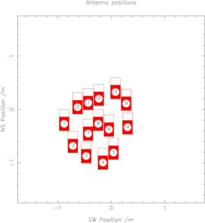
Figure 1: Left: The array design used for the compact array. Right: The resulting $uv$-coverage for a 6-hour observation.

The measurement of primordial structure in the cosmic microwave background (CMB) is of great importance in cosmology. These features, imprinted at $z\sim 1000$, enable direct investigation of the formation of structure in the universe as well as constraining the values of basic cosmological quantities such as the amounts of various forms of matter and vacuum energy in the universe. Primordial CMB fluctuations, however, are extremely faint ($\Delta T<100\mu$K) and have to be seen through various foregrounds and in the presence of the systematic errors inevitably present in any experiment.

These challenges account for the gap of nearly three decades between the discovery of the CMB (Penzias & Wilson, 1965) and the detection of primordial fluctuations by the COBE satellite (Smoot et al., 1992). COBE detected statistical anisotropy on angular scales of $90^{\circ}$ to $10^{\circ}$ (corresponding to angular multipoles $\ell=2$ to $20$); this is greater than the horizon scale at the epoch of imprinting and provided very strong evidence for a period of inflation in the early universe. After COBE, observations have focused increasingly on the angular scales at which features due to acoustic oscillations in the primordial plasma were expected (Sakharov, 1965; Sunyaev & Zel’dovich, 1970; Peebles & Yu, 1970).

Recently, results have been announced from a new generation of instruments capable of detecting a range of acoustic modes. As well as unequivocally detecting the first acoustic peak at $\ell\sim 220$, MAXIMA (Lee et al., 2001), BOOMERanG (Netterfield et al., 2001) and DASI (Halverson et al., 2002), all detect power at smaller angular scales, $300<\ell<800$, with strong evidence for a second peak at $\ell\sim 550$, while CBI (Padin et al., 2001) (which is optimised for observation at high $\ell$) detects the sharp decline in power at $\ell\sim 1000$ expected from photon diffusion (Silk, 1968).

Here we report measurements of the CMB anisotropies on scales of $3\aas@@fstack{\circ}6$–$0\aas@@fstack{\circ}4$ (angular multipoles $\ell$=150–900) at 34 GHz using the Very Small Array (VSA). This paper is the second in a series of four papers which report the results of the first season of observations made using the VSA in its compact configuration. Here we describe the observational strategy, data reduction and image-plane analysis, whilst Watson et al. (2002) (hereafter Paper I) provide a detailed description of the experimental method and design. Extraction of the angular power spectrum is presented by Scott et al. (2002) (Paper III), and estimates of the cosmological parameters using the VSA data are given by Rubiño-Martin et al. (2002) (Paper IV). A detailed description of the telescope will be given by Rusholme et al. (in prep.) (Paper 0).

2 OBSERVATIONS

Table 1: VSA field positions and total effective integration time remaining after flagging and filtering of the data.

	RA (J2000)	DEC (J2000)	Total Effective Integration Time (hrs)
VSA1	00 22 37.3	30 16 38	193
VSA1A	00 09 55.8	30 33 12	226
VSA1B	00 15 25.9	28 04 40	68
VSA2	09 37 57.0	30 41 29	271
VSA2-OFF	09 47 15.2	30 41 05	226
VSA3	15 39 39.3	44 50 21	187
VSA3A	15 30 35.1	42 37 49	206
VSA3B	15 46 20.8	42 22 15	119

The VSA is a development of the Cosmic Anisotropy Telescope (CAT) (Robson et al., 1993), a three-element interferometer which operated at 15 GHz from a sea-level site in Cambridge. The VSA has 14 horn-reflector antennas mounted on a tilt-table and operates over the frequency range 26–36 GHz with an observing bandwidth of 1.5 GHz. The telescope is sited at the Teide Observatory, Tenerife at an altitude of 2400m.

Prior to our first season of CMB observations, a series of commissioning observations was undertaken (see Paper I). These demonstrated that the telescope was working to specification and that systematic effects such as the effects of the Sun and the Moon can all be removed from the data to a very low level. Calibration of the data was shown to be limited only by the uncertainty in the absolute flux measurement of our primary calibrator, Jupiter, which is 3.5 %; the absolute flux calibration of VSA observations is based on the flux scale of Mason et al. (1999) and the brightness temperature of Jupiter at 34 GHz is taken to be 154.5 K.

Detailed descriptions of the VSA, its data analysis procedures and commissioning observations are given in Rusholme et al. (in prep.) and Paper I; in this paper we describe the key features of the first season’s observation of the CMB.

2.1 Array configuration

The 14 VSA antennas can be placed anywhere on the tilt-table, allowing freedom to design the array configuration for specific observational goals. The ‘compact array’ configuration used for the observations reported in this paper was optimised to provide almost uniform $uv$-coverage over the multipole range $\ell\sim 150$ – $900$, whilst minimising the number of visibilities with low fringe rates. The sky signal in such visibilities cannot be separated from the spurious signal (see Paper I), and is predominantly contributed by the shortest north-south baselines. Figure 1 shows the VSA ‘compact array’ configuration and $uv$-coverage.

2.2 Observing frequency

The VSA has the flexibility to observe anywhere in the 26–36 GHz range, with 1.5 GHz instantaneous bandwidth. This tunability allows the VSA to observe at more than one frequency. In principle, this allows one to fit for a component of a known spectral index, i.e. it would allow a separation of one or more Galactic components by virtue of their spectral indices. We have in fact chosen to observe at just a single frequency of 34 GHz. Our knowledge of the CMB foregrounds suggests that the Galactic foregrounds at frequencies $\approx 30$ GHz will contribute a few $\mu$K of signal in our fields (see section 3.2). Choosing a frequency at the higher end of the VSA observing band (34 GHz) reduces the free-free and synchrotron foregrounds by a factor of $1.8-2.2$ compared to the lower end ($\sim 26$ GHz). Since the proposed spinning dust component is expected at $\sim 15-20$ GHz (Draine & Lazarian, 1998), its 34-GHz emission also will be considerably lower than its peak value.

2.3 Field selection

For practical CMB observation, it is important to choose fields which are relatively free from Galactic and extragalactic foregrounds. All the VSA fields are situated at Galactic latitudes greater than 20^∘ and have low Galactic synchrotron and free-free emission, as predicted by the 408-MHz all-sky radio survey of Haslam et al. (1982). The dust maps of Schlegel et al. (1998) were used to select fields with relatively low dust contamination. The actual level of Galactic contamination in our fields is discussed in Section 3.2.

To avoid bright clusters, we consulted the NORAS (Bohringer et al., 2000), BCS (Ebeling et al., 1998) and Abell (Abell, 1958) catalogues. All fields were also chosen to be as free as possible of bright radio sources, since these are the major contaminant of CMB observations at 34 GHz. We used two low-frequency surveys, NVSS (Condon et al., 1998) at 1.4 GHz and Green Bank (Gregory et al., 1996) at 4.85 GHz to select CMB fields in which there were predicted to be no sources brighter than 500 mJy at 34 GHz within the VSA primary beam (FWHM$=4\aas@@fstack{\circ}6$). Predictions were made by extrapolating the flux density of every source in the 4.8 GHz catalogue to 34 GHz using its spectral index between 1.4 and 4.85 GHz. A further practical consideration which affected the choice of CMB fields was the need to observe all fields for a reasonable length of time (more than 5 hours) from both Tenerife and Cambridge. This limits the declination range of our fields to between +26^∘ and +54^∘. To maximize observing efficiency, we also selected fields that are evenly spaced around the sky. In order to increase the $\ell$-resolution of our measurement of the CMB power spectrum, we selected regions of sky where we can mosaic several VSA pointings. In each region of sky, mosaiced fields are separated by $2\aas@@fstack{\circ}75$. Our final choice of fields used during the first year of observation is shown in Figure 2 and in Table 1.

2.4 Observing strategy

During the first year of VSA observations, we undertook two distinct observation programmes, each using the compact array. First, we have made deep mosaiced observations of eight fields in three evenly spaced regions of sky (hatched regions in Figure 2). Each mosaiced field was observed for $\sim$ 400 hours, reaching a thermal noise of approximately 30 mJy. Mosaicing in this way enables us to increase the $\ell$-resolution of our measurements whilst also reducing sample variance. However, all the fields must be observed with the Ryle Telescope in Cambridge for source subtraction (see section 3.5), and the time taken for us to survey all fields with the Ryle Telescope prior to any observation with the VSA has limited the area of sky that we can cover with deep mosaicing in this first year. Consequently, for $\ell\leq$ 300, our measurements of the CMB power spectrum are limited by sample variance.

In order to achieve a good estimate of the CMB power spectrum in the region $\ell\leq$ 300, we undertook a second observation programme; a shallow survey in one large area of sky. The shallow survey consists of 2 days observation on each of 30 mosaiced fields (Figure 2 hexagonal region), and covers an area of approximately 300 square degrees. For this shallow survey, our source subtraction strategy no longer limits the area of sky we can observe with the VSA in a given time. Since for the shallow survey we are only concerned with low-$\ell$ observations, where the contribution of point sources to the CMB power spectrum will be negligible, prior surveying with the Ryle Telescope is not necessary. Instead, we monitor only sources predicted to be greater than 100 mJy at 34 GHz on the basis of low-frequency survey information. Only the results from the deep mosaiced fields are reported in this series of VSA results papers; the results from the shallow survey will be presented in a later paper.

2.5 Observing schedule

Quasi-independent tracking of the VSA antennas enables us to effectively filter out the effects of bright contaminating sources such as the Sun and the Moon (see Paper I). We are able therefore to observe during both the day and night, with useful CMB observations possible at separations as close as 40 degrees from the Sun and 30 degrees from the Moon. Consequently, we implemented an observing strategy that made use of all available time during the first year of observation.

In each 24-hour period, we obtained 5–6 hours of integration on each of 3 CMB fields; the total effective integration time (after flagging and filtering of the data) for each of the VSA fields is given in Table 1. The remaining time in each 24-hour period was divided between calibration sources. We observed at least one flux calibrator (Jupiter, Cas A or Tau A), with observations of fainter sources (e.g. NGC7027, 3C273 and Cyg A) interspersed. Observation of fainter sources allowed valuable checks on the diurnal stability of the telescope.

Figure 2: Plot of the VSA fields observed during our first year of observations, projected on to the equatorial plane. The hatched regions are fields which were observed using deep mosaicing, the results of which are the subject of this series of papers. The remaining fields were observed as part of a shallow survey and are not discussed further here. Radio sources predicted to be brighter than 500 mJy at 34 GHz are displayed as star symbols. A cut-off at Galactic latitude $|\rm b|>$ 20^∘ has been applied.

2.6 Data reduction

The data from the first year of VSA observations were reduced as described in detail in Paper I. Each day’s CMB observation is reduced and analysed independently. The resulting calibrated visibilities from each day are stacked together, and the full dataset for each field is analysed. We check the stacks by eye for signs of residual contaminating signal, which is easily identified as regions of coherent phase. The data are stacked both as a function of hour angle and per-antenna, and are flagged interactively. This stage of flagging typically removes 20$\%$ of the data; this is in addition to the preliminary flagging operations described in Paper I, which account for abnormal errors such as pointing, hardware failure, bad weather and filtering of the spurious signal.

The fully-flagged and stacked data are held as visibility files, containing the real and imaginary part for each observed $uv$-position along with an associated rms noise level. It is critical for the power spectrum analysis that the estimate of the noise on each visibility is accurate. We calculate the noise on each visibility point from the scatter in the visibility data on each baseline each day. This takes into account the number of flagged points in each smoothed 64-second sample, in addition to other flagging operations such as gain corrections implied by the system temperature monitoring. As a further check, we recalculate our noise estimates when the data are gridded in the $uv$-plane, prior to producing reduced datasets for the power spectrum estimation. Here we estimate the noise for each gridded visibility using the spread of values within the stacked files (i.e. using the complete 70–80 day data sets). Both methods yield the same noise estimates.

The final data stacks for each of the VSA fields typically contain $\simeq$ 800,000 visibility points, each one averaged over 64 seconds. The combined edits from all categories result in a rejection of $\simeq$ 50$\%$ of the data in each field.

3 FOREGROUNDS

Table 2: Galactic foreground contamination for the 3 VSA mosaiced fields at 1^∘ resolution. The rms estimates are in $\mu$K, and are calculated for 34 GHz.

Component	Template / assumptions	VSA1	VSA2	VSA3
Synchrotron	Haslam 408 MHz	2.2	1.2	1.0
	$\beta=3.0$
Free-free	WHAM H$\alpha$	0.8	0.8	0.6
	1R=4.5$~{}\mu$K
Spinning Dust	Schlegel et al. 100 $\mu$m	5.0	1.4	2.4
	1 MJy sr-1 = 10 $\mu$K
Total (estimated)	uncorrelated	5.5	2.0	2.7

3.1 Diffuse Galactic foregrounds

The diffuse Galactic foregrounds consist of three known components: synchrotron, free-free and vibrational dust, together with a further postulated component of spinning dust.

Synchrotron emission has a varying spectral index ($T\propto\nu^{-\beta}$) of $\beta_{synch}\approx 2.7-3.2$ (Davies et al., 1996) depending on frequency and position on the sky. The steep spectral index allows low-frequency radio surveys such as the 408-MHz all-sky radio map (Haslam et al., 1982) and the 1420-MHz radio map (Reich & Reich, 1988) to be used to estimate the synchrotron component at higher frequencies.

Free-free emission is thermal bremsstrahlung radiation emitted by ionized gas in the Galaxy. The spectral index for free-free is more well-known with $\beta_{ff}\approx 2.15$; it shows very little variation with electron temperature and density, although it does steepen slightly at higher frequencies. The 656.3 nm H$\alpha$ line is a good tracer of free-free emission (Valls-Gabaud (1998) and Dickinson et al. in prep). Dust absorption, however, can cause these estimates to be systematically lower than the true values.

Vibrational dust is only a concern for CMB experiments observing at frequencies above $\sim 90$ GHz (de Zotti et al., 1999), and is expected to contribute $<<1~{}\mu$K at VSA observing frequencies. A further component has recently been postulated by Draine & Lazarian (1998), based on observational evidence (Kogut et al. (1996); Leitch et al. (1997); de Oliveira-Costa et al. (1997); de Oliveira-Costa et al. (1999); de Oliveira-Costa et al. (2002), but see also Mukherjee et al. (2001)). They postulate a population of ultra-small ($\sim 10^{-9}$m) spinning dust grains which emit via rotational emission. The spectrum of spinning dust is likely to be highly peaked at about $15-20$ GHz.

3.2 Galactic foregrounds in the VSA fields

A simple method of estimating the foreground contamination is to calculate the rms variation in each of the foreground template maps for each VSA field. This is then converted to temperature units at 34 GHz. This is simplistic and susceptible to uncertainty due to the extrapolation to 34 GHz. This method, however, does give us an estimate of the amplitude of the foreground signals and indicates to what level the VSA observations are contaminated by diffuse foregrounds. A more rigorous cross-correlation analysis will be presented in a future paper (Dickinson et al., in prep.).

The rms method has been applied to $8^{\circ}\times 8^{\circ}$ patches of sky centred on each of the three VSA deep fields (VSA1, VSA2 and VSA3). These are large enough to cover the mosaiced fields within the $4\aas@@fstack{\circ}6$ FWHM of the primary beam. We use the de-striped and source-subtracted version of the Haslam et al. (1982) 408 MHz map as used by Davies et al. (1996) to trace the synchrotron component, whilst the recently published WHAM H$\alpha$ data (Reynolds et al., 1998) are used to trace the free-free component. For the dust-correlated emission, we use the 100 $\mu$m IRAS/DIRBE map given by Schlegel et al. (1998). The maps were smoothed to $1^{\circ}$ resolution since the WHAM data are at $\sim 1^{\circ}$ resolution.

The synchrotron emission is assumed to have a spectral index $\beta=3.0$ between 408 MHz and 34 GHz. The conversion from H$\alpha$ units (1 Rayleigh $(R)\equiv 10^{6}/4\pi$ photons s^-1 cm^-2 sr^-1) to free-free emission is calculated to be 4.5 $\mu$K/$R$ (Dickinson et al. in prep.). To estimate the $total$ dust-correlated component (which may include emission from spinning dust and vibrational dust) we have assumed a coupling coefficient of 10 $\mu$K/(MJy sr^-1). This number is rather arbitrary since previous estimates which range from $0-36\mu$K/(MJy sr^-1) at $\approx 30$ GHz, have been calculated for different angular scales and for different regions of sky. The total value is the sum of the individual components added in quadrature. The estimates of the components and total contamination from Galactic foregrounds for the three fields are given in Table 2.

The value of the synchrotron component is probably an over-estimate since there are some residuals from discrete radio sources left in the map; above $\sim$ 10 GHz, the free-free component is expected to dominate the synchrotron component. The free-free estimate from H${\alpha}$ is probably the most reliable although there may be some absorption of the H$\alpha$ signal due to dust. Following Dickinson et al. (in prep.), we can use the 100 $\mu$m emissivity to calculate what this correction might be. For all the VSA fields, the dust emissivity is $<5$ MJy sr^-1. If all the dust were lying in front of the H$\alpha$ gas, then the correction is $23$ percent. A more likely situation is a mixing of the gas and dust, thus the dust correction is $\sim$ 10 percent. The table indicates the brightest Galactic foreground may be the spinning dust, although very little is known about this component. The estimates are likely to be higher than the real value since we chose a rather high coupling coefficient based primarily on the COBE-DMR dust-correlated value (Kogut et al., 1996) which is only strictly true at the 7^∘ scale. This is the total dust correlated component which will also include any other correlated foreground, most notably, the free-free component.

In summary, using rms estimates for these VSA fields, it seems that the diffuse Galactic foregrounds are very weak at 34 GHz compared to the primordial CMB signal. For example, if $T_{\rm CMB}=60~{}\mu$K near the first peak $\ell\sim 200$ and $T_{\rm GAL}=5~{}\mu$K, then the contamination is at the $0.35$ per cent level. For $\ell\sim 800$, if $T_{\rm CMB}=30~{}\mu$K, then the contamination is $1.4$ per cent. However, the contamination is likely to be considerably smaller at higher $\ell$-values, since all the Galactic foregrounds have power spectra which decrease at smaller angular scales. The full cross-correlation analysis (Dickinson et al., in prep.) will provide a more accurate estimate of the contamination from Galactic foregrounds.

3.3 Point sources

Radio sources (mostly radio galaxies and quasars, but also some stars) are expected to be a major contaminant of CMB observations at centimetre wavelengths (see e.g., Taylor et al. (2001)). Their population is not well known at frequencies higher than 10 GHz, and many are expected to be variable and/or have spectra that rise with frequency, i.e. $\alpha<0$ (where flux density S $\propto\nu^{-\alpha}$). On the angular scales of interest to primordial CMB work, such sources are also generally unresolved. To eliminate point source contamination from VSA observations, all the radio sources in each CMB field with flux density greater than our source-confusion limit, are observed and subtracted directly from our visibility data. We estimate the contribution of unsubtracted sources below our confusion limit using a preliminary estimate of the 34 GHz source count; this source count is estimated from the sample of sources we detect at 34 GHz.

Table 3: Point sources subtracted from VSA fields. The apparent flux is the flux of each source at 34 GHz as observed by the VSA (i.e. including the effect of the VSA primary beam). This flux represents the actual flux subtracted from each map.

	RA (J2000)	DEC (J2000)	Apparent Flux (Jy)
VSA1	00 10 27.7	28 54 58	0.028
	00 15 06.1	32 16 13	0.155
	00 19 39.7	26 02 53	0.043
	00 23 39.6	29 28 29	0.091
	00 24 34.3	29 11 31	0.088
	00 28 17.0	29 14 29	0.054
	00 34 43.4	27 54 26	0.037
	00 36 59.7	29 58 59	0.029
	00 41 15.9	32 11 08	0.011
VSA1A	23 55 44.0	30 12 42	0.018
	00 10 27.7	28 54 58	0.058
	00 12 47.3	33 53 36	0.029
	00 13 44.0	34 41 42	0.008
	00 15 06.1	32 16 13	0.167
	00 15 37.9	33 32 41	0.017
	00 19 37.7	29 56 02	0.033
	00 23 39.6	29 28 29	0.019
	00 24 34.3	29 11 31	0.020
VSA1B	00 00 35.1	29 14 29	0.019
	00 00 55.9	25 16 24	0.014
	00 01 21.5	25 26 51	0.015
	00 03 16.3	24 59 42	0.008
	00 04 34.5	29 46 18	0.021
	00 06 48.8	24 22 38	0.027
	00 12 38.1	27 02 40	0.057
	00 15 06.1	32 16 13	0.033
	00 16 03.6	24 40 18	0.025
	00 18 12.4	29 21 25	0.101
	00 19 39.7	26 02 53	0.298
	00 19 52.4	26 47 31	0.052
	00 23 23.0	25 39 19	0.044
	00 34 43.4	27 54 26	0.015
VSA2	09 23 48.0	31 07 56	0.047
	09 23 51.5	28 15 26	0.047
	09 25 43.6	31 27 11	0.062
	09 32 55.0	33 39 29	0.023
	09 39 01.6	29 08 29	0.055
	09 41 48.1	27 28 38	0.051
	09 52 06.1	28 28 31	0.011
	09 53 27.9	32 25 52	0.012
	09 58 20.9	32 24 02	0.014

Table 4: continued

	RA (J2000)	DEC (J2000)	Apparent Flux (Jy)
VSA2-OFF	09 27 39.8	30 34 16	0.060
	09 31 51.8	27 50 52	0.013
	09 37 06.3	32 06 55	0.026
	09 41 48.1	27 28 38	0.035
	09 41 52.3	27 22 18	0.018
	09 42 36.1	33 44 37	0.017
	09 52 06.1	28 28 31	0.031
	09 53 27.9	32 25 52	0.053
	09 54 39.7	26 39 23	0.006
	09 55 37.9	33 35 03	0.018
	09 58 20.9	32 24 02	0.267
	09 58 58.9	29 48 04	0.026
	10 00 07.5	27 52 45	0.012
	10 01 10.1	29 11 38	0.043
	10 01 46.2	28 46 55	0.028
VSA3	15 21 49.5	43 36 39	0.106
	15 39 42.4	43 37 41	0.089
	15 45 08.4	47 51 54	0.021
	15 56 36.1	42 57 07	0.018
	15 57 18.9	45 22 21	0.022
VSA3A	15 06 52.9	42 39 22	0.056
	15 11 42.6	44 30 44	0.010
	15 16 31.4	43 49 49	0.023
	15 17 56.9	39 36 40	0.016
	15 19 26.9	42 54 08	0.066
	15 20 39.6	42 11 12	0.043
	15 21 49.5	43 36 39	0.238
	15 26 45.3	42 01 41	0.081
	15 36 13.7	38 33 27	0.014
	15 36 23.1	38 45 52	0.011
	15 38 55.7	42 25 27	0.065
	15 42 58.9	45 45 59	0.012
	15 45 21.3	41 30 27	0.026
	15 47 58.9	42 08 52	0.021
VSA3B	15 21 49.5	43 36 39	0.017
	15 57 18.9	45 22 21	0.012
	16 08 22.0	40 12 15	0.010

3.4 Source confusion and the VSA

The level to which sources must be subtracted from our CMB fields is determined by comparing the flux sensitivity of the VSA to the rms confusion noise remaining from unsubtracted sources. The VSA, operating in its compact configuration, has a flux sensitivity of about 30 mJy in each deep mosaic pointing. In order that our observations are dominated by receiver noise we must therefore ensure that the rms flux density on a VSA map from unsubtracted sources, the confusion noise, is less than the flux sensitivity of 30 mJy. Following the standard approach (e.g. Scheuer (1957)),

$$\sigma^{2}_{\rm conf}=\Omega\int_{0}^{S_{\rm sub}}n(S)S^{2}dS,$$

where $S$ is the flux density, $n(S)$ is the differential source count per steradian, $\Omega$ is the VSA synthesised beam solid angle and $S_{sub}$ is the flux density limit down to which sources are subtracted. Normalising this in terms of the number of sources, $N$, per VSA synthesised beam that are subtracted,

$$N=\int_{S_{\rm sub}}^{\infty}\Omega n(S)dS,$$

and parameterising $n(S)$ as $n(S)dS=KS^{-\beta}$, we obtain

$$\sigma_{\rm conf}=[N(\beta-1)/(3-\beta)]^{1/2}S_{\rm sub}.$$

For a given level of source subtraction, $S_{\rm sub}$, one can thus estimate the residual confusion noise. The level of source subtraction can then be optimised to ensure that $\sigma_{\rm conf}$ is less than the flux sensitivity of the VSA. To calculate this confusion noise, however, the differential source count, $n(S)$, at our observing frequency of 34 GHz is required. At the outset of observations with the VSA, the source count at 34 GHz was not known. Instead we used an estimate extrapolated from the 15-GHz source count obtained using source subtraction observations for the Cosmic Anisotropy Telescope(CAT).

Based on the small sample of sources observed during the CAT source-subtraction program, the 15 GHz source counts were found to have $\beta=-$1.8 (O’Sullivan, 1995). Using this value for $\beta$ at 15 GHz and assuming a conservative average spectral index of $\alpha$=0 between 15 and 34 GHz, we find that to ensure that the confusion noise is significantly lower than the flux sensitivity of the VSA ($\simeq$ 30 mJy) we must subtract all sources brighter than 80 mJy at 34 GHz.

Table 5: This table gives the thermal noise level,in mJy beam^-1, for each VSA field, measured both from standard and autosubtracted maps (see text for explanation). The rms noise level in the centre of each map and the corresponding residual CMB signal observed in each field, in mJy, is also given. These values are taken from CMB maps made at full resolution. The approximate flux-to-temperature conversion is $\rm 1\,mJy\,beam^{-1}\equiv 1.1\,\mu K$, giving mean rms CMB fluctuations in the maps of 40 – 65 $\mu$K.

	Thermal Noise	Thermal Noise	RMS Noise	CMB Signal
	(standard map)	(autosubtracted map)	in centre of map
VSA1	37	38	52	37
VSA1A	46	43	51	27
VSA1B	60	63	81	55
VSA2	39	37	70	58
VSA2-OFF	34	33	53	41
VSA3	39	39	56	40
VSA3A	36	39	63	52
VSA3B	50	49	75	56

3.5 Source-subtraction strategy

To ensure that all potentially contaminating sources are detected, one would ideally survey each CMB field at the same frequency as the VSA, but with increased resolution and sensitivity. This, however, would require a telescope more expensive than the VSA. Instead, we adopt a two-stage strategy.

First, prior to observation with the VSA, we survey all the VSA fields at 15 GHz using the Ryle Telescope (RT) in Cambridge. The RT, which uses five 13-m diameter antennas and gives a resolution of $\simeq 30$ arcsecs, is used in a raster scanning-mode and reaches an rms noise level of $\sigma\simeq 4$ mJy (see Waldram et al. (2002)). This allows us to identify sources above 20 mJy at 15 GHz, and ensures that we find all sources above our source-confusion limit of 80 mJy at 34 GHz, even allowing for a spectral index as steep as $\alpha\simeq$ $-$2 between 15 and 34 GHz.

Having identified the contaminating sources in each field, we monitor each source at 34 GHz using a separate single-baseline interferometer working simultaneously with the VSA (see Paper I). This single-baseline interferometer consists of two 3.7-m dishes separated by 9 metres on a north-south baseline. Each dish is situated in an enclosure similar to that of the VSA, and is fitted with identical horn-reflector feeds and receivers as used on the main array. All sources identified in the 15 GHz survey are monitored. The monitoring is done simultaneously with and at the same frequency as the VSA observation, ensuring that sources which are variable on time-scales as short as a few days can be subtracted accurately.

On average, each source identified in the 15-GHz survey is observed once every three days. The flux of each monitored source is then averaged over the duration of each corresponding field observation (typically 80 days) and its contribution is then subtracted directly from the stacked visibility data.

3.6 Point source observations

In total, 346 sources with flux densities greater than 20 mJy were identified in the 15 GHz survey of the VSA fields. All of these sources were observed with the source subtractor, and the list of monitored point sources with flux densities greater than 60 mJy at 34 GHz is given in Table 3. Although our source-subtraction strategy requires that only sources brighter than 80 mJy must be subtracted, and our source list is only complete to this level, since the data were available we subtracted point sources down to a flux limit of 60 mJy. Typically, between 10 and 15 sources with flux density greater than 60 mJy were subtracted from each CMB field.

To calculate the residual point-source contamination remaining after source-subtraction, we used a preliminary source count at 34 GHz. The source count is based on the 78 sources with $S_{34}>60$ mJy detected by the source subtractor. The differential count is given approximately by

$$\frac{{\rm d}N}{{\rm d}S}=54\left(\frac{S}{\rm Jy}\right)^{-2.15}\,{\rm Jy}^{-1}{\rm sr}^{-1}.$$

Note that this count is not entirely accurate due to the uncertain completeness at lower flux levels, but is sufficient to estimate our residual confusion noise. A more complete analysis of the 34-GHz count will be given in a subsequent paper. When the count is integrated up to our nominal subtraction limit of 80 mJy it gives a residual confusion noise of $\sigma_{\rm conf}=14$ mJy, which when added in quadrature to our typical thermal noise of 40 mJy gives only a 6 % increase in noise level. The effect of the residual sources on the CMB power spectrum is discussed in Paper III.

4 RESULTS

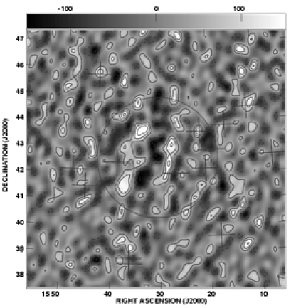
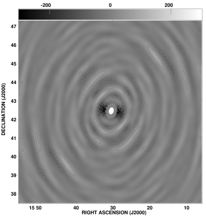
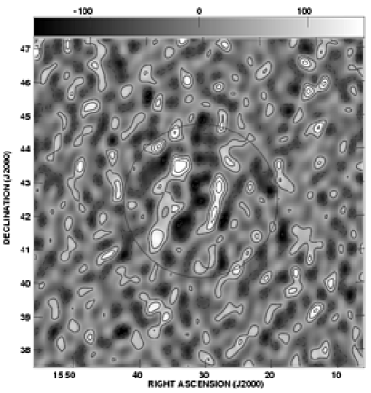
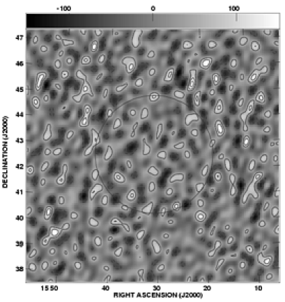
Figure 3: Maps of a sample VSA field (VSA3A) at full resolution. Top left: the map before source subtraction. Positions of sources to be subtracted are marked with crosses, and the FWHM of the primary beam is indicated by a circle. CMB fluctuations (and some sources) are clearly visible within the primary beam. Top right: the synthesised beam of all the images. Bottom left: the map after source subtraction. Bottom right: the autosubtracted map (see text), showing the uniform noise level across the map. In all maps the greyscale runs from -150 to 150 mJy beam^-1 and the contour interval is 50 mJy beam^-1; in the beam the greyscale is -0.3 to 0.3 and the contour interval is 5% of the peak.

Although the CMB power spectrum is calculated directly from the complex visibility data obtained from our observations (see Paper III), image-plane analysis provides valuable consistency checks on the data. Here we present images of the VSA fields and discuss the checks that we have performed on the data.

Figure 3 shows images of a typical VSA individual field (VSA3A) at full resolution. The top two panels show the map before source-subtraction and the synthesised beam, while the lower left panel shows the map after source subtraction. Inside the primary beam envelope (FWHM = 4$\aas@@fstack{\circ}$6, shown by a circle), the maps are dominated by astronomical signal. Outside this region, the maps are dominated by instrumental (thermal) noise.

Comparison of the rms power measured in the outer region of each map with the calculated instrumental noise provides information about the level of residual contaminating signals. Unwanted signals (such as crosstalk or distant bright sources) are not constrained to lie within the primary beam envelope in the image plane. Instead their effect is to increase the total rms power level across the whole of a map. A simple way to measure the instrumental noise directly from a map is to measure the rms level far from the primary beam. The measured noise levels, given in Table 5, all agree extremely well with the calculated values. The slightly higher noise levels obtained in VSA1B and VSA3B reflect the smaller amount of data collected on these fields.

A more rigorous approach to estimating the thermal noise on each map, and also the amount of any residual contaminating signal, is to ‘autosubtract’ our visibility data. Here we take the time-ordered visibility data for each field and reverse the sign of alternate visibilities. On the time scale between adjacent visibility points (64 seconds), both astronomical and spurious signals are effectively coherent, and are thus cancelled out. In contrast, the noise on adjacent visibilities is completely uncorrelated, and the rms noise on the map is unaffected. This technique therefore provides a robust estimate of our thermal noise. In addition, we can compare the rms power in the autosubtracted maps with that far outside the primary beam envelope of our standard field maps. Any discrepancy between the two would be indicative of residual spurious signals.

Autosubtraction was applied to all eight VSA fields, and maps of each field were made. The bottom right panel in Figure 3 shows the autosubtracted map for VSA3A. Clearly the astronomical signal has been subtracted, leaving a constant noise level. The rms noise on each autosubtracted map was measured and the values are given in Table 5. There is excellent agreement between the noise levels measured far from the map centres and those measured by autosubtraction.

The approximate CMB signal level in each map can be estimated by subtracting the map rms in the central area ($4\times 4$ degrees) in quadrature from the rms noise level estimated from the autosubtracted maps (or from the far-out portions of the sky maps). These figures are also given in Table 5, and represent the average temperature fluctuations in the CMB averaged over the $\ell$-range of the observations. For the synthesised beam size of the full resolution maps ($\simeq 17$ arcmin), the approximate flux-to-temperature conversion is $\rm 1\,mJy\,beam^{-1}\equiv 1.1\,\mu K$, giving mean rms CMB fluctuations in the maps of 40 – 65 $\mu$K.

All the maps are robust to minor variations in flagging and filtering. The data have also been split by observing epoch, by day/night and by alternate visibilities; the resulting maps are fully consistent with each other. Analogues of theses consistency checks are also applied to the power spectra (see Paper III).

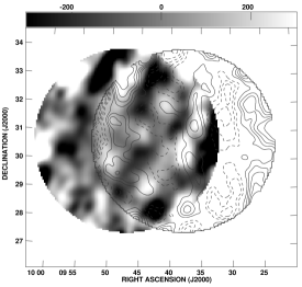
Figure 4: Comparison of the overlapping region in the VSA2 mosaic. A contour map of VSA2-OFF is overlayed on a greyscale image of VSA2. Structures common in both position and flux level are visible. Both maps were made with a taper corresponding to the CMB power spectrum to maximise the signal-to-noise, have been corrected for the primary beam response of the VSA, and are truncated at the 25% point of the primary beam. The grey scale runs from $-300$ to $300$ mJy beam^-1 and the contour interval is 150 mJy beam^-1.

In addition to analysing each field independently, it is instructive to compare images of fields within each mosaiced region. As an example, we present an image of the VSA2/VSA2-OFF mosaic (Figure 4). Here a contoured map of VSA2-OFF is overlaid on a grey-scale image of the VSA2 field. Common structures are clearly seen, agreeing in both position and in flux density.

Finally, in Figure 5, we present images of the fully source-subtracted VSA fields. To enhance signal-to-noise, a $uv$-taper function has been applied to the data. The taper has the form of the CMB power spectrum estimated from the complete VSA data set (see Paper III). The individual overlapping maps are combined linearly using standard Aips tasks. The individual maps are transformed to the same grid, then corrected for the individual primary beam responses (which multiplies up the outer parts of the map); they are then combined pixel by pixel, weighted by their primary beams, and the resulting image multiplied by the total weight map, resulting in an image in units of signal-to-noise. This is then re-scaled back to the map units of Jy beam^-1. (This final re-scaling is only approximate as the sensitivities vary slightly between the component maps; however, no quantitative analysis is done using these images). The peak value of the signal-to-noise varies between 6 and 8.5 in the three combined images. The maps have not been CLEANed, so the CMB fluctuations are convolved with the synthesised beam, which is somewhat different for each field due to differences in flagging.

5 CONCLUSIONS

We have observed eight overlapping fields in three separate regions of the sky with the VSA compact array, a total of 101 square degrees. The CMB anisotropies are clearly detected in all fields, and individual features in different overlapped pointings agree well with each other. We have assessed the Galactic foreground contamination based on low-frequency radio, dust, and ${\rm H}_{\alpha}$ data, and found it to be negligible. To eliminate confusion by foreground radiosources, we have surveyed all the fields at 15 GHz with the Ryle Telescope (RT). The flux of all sources found in the RT survey were monitored simultaneously with and at the same frequency as the VSA observations using a separate single-baseline interferometer. These sources were subtracted from the data. The count of sources in the VSA fields is effectively complete to 80 mJy at 34 GHz, although we have detected sources as faint as 60 mJy. After removal of these sources from the VSA main array data, the residual source confusion is negligible. We have checked the data for evidence of components other than the CMB and thermal noise, and have found none.

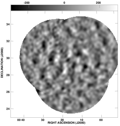
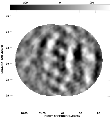
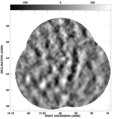
Figure 5: Images of the three VSA regions, with radio sources subtracted. The individual maps were made with a radial taper applied to the visibilities in order to enhance the signal-to-noise of the CMB features, then combined using the Aips tasks ltess and stess. These form a linear combination of the component maps, weighted by the individual primary beam responses. The point-spread function (or synthesised beam) have not been deconvolved from these images, which thus have correlations across them. Differing aperture plane coverages due to different flagging of the data have resulted in different synthesised beams in each image. Top left: VSA1,1A and 1B. Top right: VSA2 and VSA2-OFF. Bottom left: VSA3,3A and 3B. In each case the greyscale runs from -300 to 300 mJy  beam^-1. Bottom right: The weighting function used to taper the maps in order to improve the signal-to-noise ratio, based on the power spectrum of the data; the weighting function is proportional to $C_{\ell}^{1/2}$.

References

- Abell (1958) Abell G. O., 1958, ApJS, 3, 211
- Bohringer et al. (2000) Bohringer H., et al., 2000, VizieR Online Data Catalog, 212, 90435
- Condon et al. (1998) Condon J. J., Cotton W. D., Greisen E. W., Yin Q. F., Perley R. A., Taylor G. B., Broderick J. J., 1998, AJ, 115, 1693
- Davies et al. (1996) Davies R. D., Gutierrez C. M., Hopkins J., Melhuish S. J., Watson R. A., Hoyland R. J., Rebolo R., Lasenby A. N., Hancock S., 1996, MNRAS, 278, 883
- de Oliveira-Costa et al. (2002) de Oliveira-Costa A. ., Tegmark M., Finkbeiner D. P., Davies R. D., Gutierrez C. M., Haffner L. M., Jones A. W., Lasenby A. N., Rebolo R., Reynolds R. J., Tufte S. L., Watson R. A., 2002, ApJ, 567, 363
- de Oliveira-Costa et al. (1999) de Oliveira-Costa A. ., Tegmark M., Gutiérrez C. M., Jones A. W., Davies R. D., Lasenby A. N., Rebolo R., Watson R. A., 1999, ApJ, 527, L9
- de Oliveira-Costa et al. (1997) de Oliveira-Costa A., Kogut A., Devlin M. J., Netterfield C. B., Page L. A., Wollack E. J., 1997, ApJ, 482, L17
- de Zotti et al. (1999) de Zotti G., Toffolatti L., Argüeso F., Davies R. D., Mazzotta P., Partridge R. B., Smoot G. F., Vittorio N., 1999, in AIP Conf. Proc. 476: 3K cosmology The Planck Surveyor Mission: Astrophysical Prospects. p. 204
- Draine & Lazarian (1998) Draine B., Lazarian A., 1998, Astrophys.J., 494, L19
- Ebeling et al. (1998) Ebeling H., Edge A. C., Bohringer H., Allen S. W., Crawford C. S., Fabian A. C., Voges W., Huchra J. P., 1998, MNRAS, 301, 881
- Gregory et al. (1996) Gregory P. C., Scott W. K., Douglas K., Condon J. J., 1996, ApJS, 103, 427
- Halverson et al. (2002) Halverson N. W., et al., 2002, ApJ, 568, 38
- Haslam et al. (1982) Haslam C. G. T., Stoffel H., Salter C. J., Wilson W. E., 1982, A&AS, 47, 1
- Kogut et al. (1996) Kogut A., Banday A., Bennett C., Gorski K., Hinshaw G., Smoot G., Wright E., 1996, Astrophys.J., 464, L5
- Lee et al. (2001) Lee A. T., et al., 2001, Astrophys.J., 561, L1
- Leitch et al. (1997) Leitch E. M., Readhead A. C. S., Pearson T. J., Myers S. T., 1997, ApJ, 486, L23
- Mason et al. (1999) Mason B. S., Leitch E. M., Myers S. T., Cartwright J. K., Readhead A. C. S., 1999, AJ, 118, 2908
- Mukherjee et al. (2001) Mukherjee P., Jones A. W., Kneissl R., Lasenby A. N., 2001, MNRAS, 320, 224
- Netterfield et al. (2001) Netterfield C., et al., 2001, A measurement by BOOMERANG of multiple peaks in the angular power spectrum of the cosmic microwave background, Accepted by ApJ, astro-ph/0104460
- O’Sullivan (1995) O’Sullivan C., 1995, PhD. Thesis,University of Cambridge
- Padin et al. (2001) Padin S., Cartwright J. K., Mason B. S., Pearson T. J., Readhead A. C. S., Shepherd M. C., Sievers J., Udomprasert P. S., Holzapfel W. L., Myers S. T., Carlstrom J. E., Leitch E. M., Joy M., Bronfman L., May J., 2001, ApJ, 549, L1
- Peebles & Yu (1970) Peebles P. J. E., Yu J. T., 1970, ApJ, 162, 815
- Penzias & Wilson (1965) Penzias A. A., Wilson R. W., 1965, ApJ, 142, 419
- Reich & Reich (1988) Reich P., Reich W., 1988, A&AS, 74, 7
- Reynolds et al. (1998) Reynolds R. J., Tufte S. L., Haffner L. M., Jaehnig K., Percival J. W., 1998, Publications of the Astronomical Society of Australia, 15, 14
- Robson et al. (1993) Robson M., Yassin G., Woan G., Wilson D. M. A., Scott P. F., Lasenby A. N., Kenderdine S., Duffett-Smith P. J., 1993, A&A, 277, 314
- Rubiño-Martin et al. (2002) Rubiño-Martin J. A., et al., 2002, First results from the Very Small Array IV: Cosmological Parameter Estimation, Submitted to MNRAS
- Sakharov (1965) Sakharov A. A., 1965, ZhETP, 49, 345
- Scheuer (1957) Scheuer P., 1957, Proc. Cambridge Phil. Soc., 53, 764
- Schlegel et al. (1998) Schlegel D. J., Finkbeiner D. P., Davis M., 1998, ApJ, 500, 525
- Scott et al. (2002) Scott P. F., et al., 2002, First results from the Very Small Array III: The CMB Power Spectrum, Submitted to MNRAS
- Silk (1968) Silk J., 1968, ApJ, 151, 459
- Smoot et al. (1992) Smoot G. F., et al., 1992, ApJ, 396, L1
- Sunyaev & Zel’dovich (1970) Sunyaev R., Zel’dovich Y., 1970, Comments Astrophys. Space Phys., 2, 66
- Taylor et al. (2001) Taylor A. C., Grainge K., Jones M. E., Pooley G. G., Saunders R. D. E., Waldram E. M., 2001, MNRAS, 327, L1
- Valls-Gabaud (1998) Valls-Gabaud D., 1998, Publications of the Astronomical Society of Australia, 15, 111
- Waldram et al. (2002) Waldram E. M., Pooley G. G., Grainge K. J. B., Jones M. E., Saunders R. D. E., Scott P. F., Taylor A. C., 2002, A Survey of Radio Sources at 15 GHz with the Ryle Telescope: Techniques and Properties , Submitted to MNRAS
- Watson et al. (2002) Watson R. A., et al., 2002, First results from the Very Small Array I: observational methods, Submitted to MNRAS