CONSTRAINTS ON $(\Omega_{\mathrm{M0}},\Omega_{\Lambda})$ FROM STRONG LENSING IN AC 114

We use a strong lensing inversion in the cluster of galaxies AC 114 to derive constraints on the cosmological parameters $\Omega_{\mathrm{M0}}$ and $\Omega_{\Lambda}$. If it is possible to measure spectroscopically the redshifts of many multiple images then one can in principle constrain ($\Omega_{\mathrm{M0}},\Omega_{\Lambda}$) through ratios of angular diameter distances, independently of any external assumptions. Numerical tests on simulated data show rather good constraints from this test. We also use an analytic “pseudo-elliptical” NFW profile in the simulations, following the general new formalism we present. An application to AC 114 favors a flat Universe, an EdS model being marginally ruled out.

1 Introduction

Several independent results seem to converge to a specific cosmological model, namely an accelerating flat Universe with $\Omega_{\mathrm{M0}}\simeq 0.3$ and $\Omega_{\Lambda}\simeq 0.7$. However, there still remain many sources of uncertainties with all methods. Thus, any other independant test to constrain the large scale geometry of the Universe is important to investigate.

Gravitational lensing has been considered as a very promising tool for such determinations. Two major methods are currently used: the statistics of gravitational lenses and the cosmic shear variance. We focus here on a measurement technique of $(\Omega_{\mathrm{M0}},\Omega_{\Lambda})$ using gravitational lensing as a purely geometrical test of the curvature of the Universe.

In the case of several sets of multiple images, it is possible in principle to constrain the geometry of the Universe, as suggested by Blandford & Narayan $\!{}^{{\bf?}}$ and analysed by Link & Pierce $\!{}^{{\bf?}}$. Following their method, we try to quantify in Sect. 2 what can be reasonably obtained on $(\Omega_{\mathrm{M0}},\Omega_{\Lambda})$ from accurate modeling of cluster-lenses, and we apply the test to AC 114.

Strong lensing effect is very sensitive to the precise projected gravitational potential. Yet, for many widespread profiles, an analytic expression cannot be derived in the elliptical case. In Sect. 3, we present a general pseudo-elliptical formalism that makes possible analytical expressions for lensing quantities. This formalism is then applied to the NFW profile.

2 Cosmological Parameters from Strong Lensing

2.1 Influence of $\Omega_{\mathrm{M0}}$ and $\Omega_{\Lambda}$ on image formation

In the lens equation $\mathchoice{\mbox{\boldmath$\displaystyle\theta_{\mathrm{S}}$}}{\mbox{\boldmath$\textstyle\theta_{\mathrm{S}}$}}{\mbox{\boldmath$\scriptstyle\theta_{\mathrm{S}}$}}{\mbox{\boldmath$\scriptscriptstyle\theta_{\mathrm{S}}$}}=\mathchoice{\mbox{\boldmath$\displaystyle\theta_{\mathrm{I}}$}}{\mbox{\boldmath$\textstyle\theta_{\mathrm{I}}$}}{\mbox{\boldmath$\scriptstyle\theta_{\mathrm{I}}$}}{\mbox{\boldmath$\scriptscriptstyle\theta_{\mathrm{I}}$}}-D_{\mathrm{LS}}/D_{\mathrm{OS}}\,\mathchoice{\mbox{\boldmath$\displaystyle\nabla$}}{\mbox{\boldmath$\textstyle\nabla$}}{\mbox{\boldmath$\scriptstyle\nabla$}}{\mbox{\boldmath$\scriptscriptstyle\nabla$}}\phi(\mathchoice{\mbox{\boldmath$\displaystyle\theta_{\mathrm{I}}$}}{\mbox{\boldmath$\textstyle\theta_{\mathrm{I}}$}}{\mbox{\boldmath$\scriptstyle\theta_{\mathrm{I}}$}}{\mbox{\boldmath$\scriptscriptstyle\theta_{\mathrm{I}}$}})$, the dependance on the cosmological parameters is solely contained in the term $E=D_{\mathrm{LS}}/D_{\mathrm{OS}}$. But with a single system of images, we can only constrain the combination $\sigma_{0}^{2}E$, where $\sigma_{0}$ is the central velocity dispersion of the lens.

If a gravitational lens shows two systems of multiple images, at redshifts $z_{\mathrm{S1}}$ and $z_{\mathrm{S2}}$, then the ratio $E(z_{\mathrm{S2}})/E(z_{\mathrm{S1}})$ does not depend on $\sigma_{0}$, so that lower order terms like $\Omega_{\mathrm{M0}}$ and $\Omega_{\Lambda}$ can be probed independently of the mass normalization. Several observational numbers have also to be gathered to derive interesting constraints. We must get spectroscopic redshifts for the lens and the sources with a good accuracy, so that $\delta z\simeq 0.001$. The positions of the different images have to be obtained very accurately, e.g. with HST images, so that $\delta\theta\simeq 0.01^{\prime\prime}$. Finally, a strong lensing inversion requires a precise modeling of the potential model, i.e. considering its type, the substructures and individual galaxies, as well as the ellipticities of the different clumps.

Under these conditions, and in a typical configuration ($z_{\mathrm{L}}=0.3$, $z_{\mathrm{S1}}=0.6$ and $z_{\mathrm{S2}}=5$), we can derive the expected error bars on the cosmological parameters in two cases (Golse et al. $\!{}^{{\bf?}}$):

$$\Lambda\mathrm{CDM}: \delta\Omega_{\mathrm{M0}}=0.3\pm 0.11\qquad\delta\Omega_{\Lambda}=0.7\pm 0.23$$ (1)

$$\mathrm{EdS}: \delta\Omega_{\mathrm{M0}}=1\pm 0.17\qquad\quad\delta\Omega_{\Lambda}=0\pm 0.48$$ (2)

However, these typical values may depend on the choice of the lens parameters and on the potential chosen to describe the lens, a problem that we investigate below.

2.2 Numerical simulations

Figure 1: Left: Multiple images generated by a pseudo-elliptical ($\epsilon=0.1$) NFW cluster at $z_{\mathrm{L}}=0.3$. Close to their respective critical lines, 3 systems of images are identified: $z_{\mathrm{S1}}=0.6$, $z_{\mathrm{S2}}=1$, $z_{\mathrm{S3}}=4$. Units are given in in arcseconds. Right: $\chi^{2}$ confidence levels (from 1-$\sigma$ to 4-$\sigma$) obtained from the optimization of the former lens configuration. The cross (+) represents the original values $(\Omega_{\mathrm{M0}}^{0},\Omega_{\Lambda}^{0})=(0.3,0.7)$.

To create a simulated lens configuration we need to fix some aritrary values of the cosmological parameters $(\Omega_{\mathrm{M0}}^{0},\Omega_{\Lambda}^{0})$. The initial data are several sets of multiple images at different redshifts, produced by the numerical code LENSTOOL (Kneib $\!{}^{{\bf?}}$). With these observables, we can recover some parameters of the potential while we scan a grid in the $(\Omega_{\mathrm{M0}},\Omega_{\Lambda})$ plane. The likelihood of the result is obtained via a $\chi^{2}$-minimization, where $\chi^{2}$ typically compares the difference in the images positions to the resolution of the field image.

An ellipticity in the gravitational potential is included in the model, using analytic lensing expressions introduced for pseudo-elliptical profiles (Sect. 3), and apply this formalism to the NFW mass profile.

With $(\Omega_{\mathrm{M0}}^{0},\Omega_{\Lambda}^{0})=(0.3,0.7)$, we generated 3 systems of multiple images (see Fig. 1). During the optimization process, we kept fixed the geometrical parameters and recovered the physical ones: the caracteristic density $\rho_{\mathrm{c}}$ and the scale radius $\theta_{\mathrm{s}}$. The corresponding confidence levels on $(\Omega_{\mathrm{M0}},\Omega_{\Lambda})$ are plotted in Fig. 1. This degeneracy is typical of our test, as shown in the many situations explored in Golse et al. $\!{}^{{\bf?}}$.

2.3 Application to the clusters of galaxies AC 114

Figure 2: Left: HST image of the center of the cluster AC 114. 3 systems of multiple images are determined. Right: $\chi^{2}$ confidence levels (from 1-$\sigma$ to 4-$\sigma$) obtained from the optimization process in AC 114.

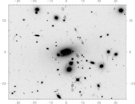
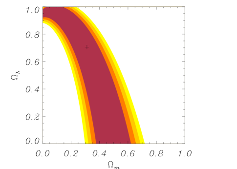
AC 114 ($z_{\mathrm{L}}=0.312$) is particularly well-suited to our test since it shows 3 systems of multiple images with spectroscopically determined redshifts : $z_{\mathrm{S1}}=1.691$, $z_{\mathrm{S2}}=1.867$ and $z_{\mathrm{S3}}=3.347$ (Campusano $\!{}^{{\bf?}}$), see Fig. 2.

We find a good fit of all these images positions by considering three main clumps, and also the individual galaxies. We use elliptical models from Hjorth & Kneib $\!{}^{{\bf?}}$ for all the components of the potential (clumps and galaxies). For the optimization, we fix all the parameters except the core radius $\theta_{\mathrm{s}}$ and the velocity dispersion $\sigma_{0}$ of the central clump. Moreover, the velocity dispersions of the galaxies and other clumps are scaled with respect to $\sigma_{0}$.

This lensing optimization of the mentionned parameters on a $(\Omega_{\mathrm{M0}},\Omega_{\Lambda})$ grid leads to the Fig. 2 confidence levels on the cosmological parameters. These rather good constraints favor a flat Universe, including the new standard one ($\Omega_{\mathrm{M0}}=0.3$, $\Omega_{\Lambda}=0.7$), as well as open models with high matter densities. Note that an EdS model is only excluded at the 1-$\sigma$ level.

3 Pseudo Elliptical Lensing Mass Model: application to the NFW profile

Cosmological $N$-body simulations of cluster formation indicate the existence of a universal density profile for dark matter halos (Navarro et al. $\!{}^{{\bf?}}$). On the other hand, gravitational lensing is an ideal tool to constrain the radial structure of collapsed halos like galaxies and clusters. Muñoz et al. $\!{}^{{\bf?}}$ introduced a general set of ellipsoidal models. However, as there are no general analytic expressions for cusped ellipsoidal models, they calculated the lensing quantities numerically. We propose a new method to introduce ellipticity in lensing models in a fully analytical way.

We introduce an ellipticity $\epsilon$ in the circular lens potential $\varphi(\theta)$. Moreover, we assume that the radial profile can be scaled by a scale radius $\theta_{s}$, thus making possible to define $x$ as $x=\theta/\theta_{s}$. We introduce the ellipticity in the expression of the lens potential by substituting $x$ by $x_{\varepsilon}=\sqrt{x_{1\epsilon}^{2}+x_{2\epsilon}^{2}}$, using the following elliptical coordinate system:

$$\left\{\begin{array}[]{lcl}x_{1\epsilon}&=&\sqrt{1-\epsilon}\,x_{1}\\ x_{2\epsilon}&=&\sqrt{1+\epsilon}\,x_{2}\\ \phi_{\epsilon}&=&\arctan\left(x_{2\epsilon}/x_{1\epsilon}\right)\end{array}\right.$$ (3)

Our method can be used if the potential $\varphi$ (and/or the deflection angle $\alpha$) and the projected mass density $\Sigma$ both have analytical expressions in the circular case. We can derive easily the corresponding convergence $\kappa_{\epsilon}(\mathchoice{\mbox{\boldmath$\displaystyle x$}}{\mbox{\boldmath$\textstyle x$}}{\mbox{\boldmath$\scriptstyle x$}}{\mbox{\boldmath$\scriptscriptstyle x$}})=\displaystyle{\kappa(\mathchoice{\mbox{\boldmath$\displaystyle x$}}{\mbox{\boldmath$\textstyle x$}}{\mbox{\boldmath$\scriptstyle x$}}{\mbox{\boldmath$\scriptscriptstyle x$}}_{\epsilon})+\epsilon\cos{2\phi_{\epsilon}}\,\gamma(\mathchoice{\mbox{\boldmath$\displaystyle x$}}{\mbox{\boldmath$\textstyle x$}}{\mbox{\boldmath$\scriptstyle x$}}{\mbox{\boldmath$\scriptscriptstyle x$}}_{\epsilon})}$ (see Golse & Kneib $\!{}^{{\bf?}}$ for more details). Similarly, the shear can be written as: $\gamma_{\epsilon}^{2}(\mathchoice{\mbox{\boldmath$\displaystyle x$}}{\mbox{\boldmath$\textstyle x$}}{\mbox{\boldmath$\scriptstyle x$}}{\mbox{\boldmath$\scriptscriptstyle x$}})=\gamma^{2}(\mathchoice{\mbox{\boldmath$\displaystyle x$}}{\mbox{\boldmath$\textstyle x$}}{\mbox{\boldmath$\scriptstyle x$}}{\mbox{\boldmath$\scriptscriptstyle x$}}_{\epsilon})+2\epsilon\cos{2\phi_{\epsilon}}\gamma(\mathchoice{\mbox{\boldmath$\displaystyle x$}}{\mbox{\boldmath$\textstyle x$}}{\mbox{\boldmath$\scriptstyle x$}}{\mbox{\boldmath$\scriptscriptstyle x$}}_{\epsilon})\kappa(\mathchoice{\mbox{\boldmath$\displaystyle x$}}{\mbox{\boldmath$\textstyle x$}}{\mbox{\boldmath$\scriptstyle x$}}{\mbox{\boldmath$\scriptscriptstyle x$}}_{\epsilon})+\epsilon^{2}(\kappa^{2}(\mathchoice{\mbox{\boldmath$\displaystyle x$}}{\mbox{\boldmath$\textstyle x$}}{\mbox{\boldmath$\scriptstyle x$}}{\mbox{\boldmath$\scriptscriptstyle x$}}_{\epsilon})-\cos^{2}{2\phi_{\epsilon}}\gamma^{2}(\mathchoice{\mbox{\boldmath$\displaystyle x$}}{\mbox{\boldmath$\textstyle x$}}{\mbox{\boldmath$\scriptstyle x$}}{\mbox{\boldmath$\scriptscriptstyle x$}}_{\epsilon}))$. Finally, the projected mass density is $\Sigma_{\epsilon}(\mathchoice{\mbox{\boldmath$\displaystyle x$}}{\mbox{\boldmath$\textstyle x$}}{\mbox{\boldmath$\scriptstyle x$}}{\mbox{\boldmath$\scriptscriptstyle x$}})=\Sigma(\mathchoice{\mbox{\boldmath$\displaystyle x$}}{\mbox{\boldmath$\textstyle x$}}{\mbox{\boldmath$\scriptstyle x$}}{\mbox{\boldmath$\scriptscriptstyle x$}}_{\epsilon})+\epsilon\cos{2\phi_{\epsilon}}(\overline{\Sigma}(\mathchoice{\mbox{\boldmath$\displaystyle x$}}{\mbox{\boldmath$\textstyle x$}}{\mbox{\boldmath$\scriptstyle x$}}{\mbox{\boldmath$\scriptscriptstyle x$}}_{\epsilon})-\Sigma(\mathchoice{\mbox{\boldmath$\displaystyle x$}}{\mbox{\boldmath$\textstyle x$}}{\mbox{\boldmath$\scriptstyle x$}}{\mbox{\boldmath$\scriptscriptstyle x$}}_{\epsilon}))$.

We apply this formalism to the NFW profile, for which both the lens potential (Meneghetti et al $\!{}^{{\bf?}}$) and the projected mass profile (Bartelmann $\!{}^{{\bf?}}$) are known analytically.

An illustration of some lensed images using is shown in Fig. 1. In particular it is possible to form a 5-image configuration. One can estimate precisely (see Golse & Kneib $\!{}^{{\bf?}}$) the range of ellipticities for which this model is a good description of elliptical mass distributions. We shall consider only $\epsilon\lesssim 0.25$, which translates to a limit of $\epsilon_{\Sigma}\lesssim 0.4$ for the projected mass density.

4 Conclusion

Following the work of Link & Pierce $\!{}^{{\bf?}}$, we discussed a method to obtain information on the cosmological parameters $\Omega_{\mathrm{M0}}$ and $\Omega_{\Lambda}$ while reconstructing the lens gravitational potential of clusters with multiple image systems at different redshifts.

This technique gives degenerate constraints, with a better precision on the matter density. The cluster AC 114, displaying 3 systems of multiple images, is well-suited for this method. The optimization process favors a flat Universe, or open ones with a high matter density.

Actually the degeneracy depends only on the different redshifts involved that we will have various sets of when applying the method to real configurations. This should lead to a more reduced area of allowed cosmological parameters, when combining data from different clusters. We plan to apply this technique to clusters like MS2137-23, MS0440+02, A370, A383 and A1689.

Strong lensing inversion requires a precise gravitational potential model. For this reason we propose a new and simple formalism that allows analytical expressions for the lensing quantities in elliptical models. We applied this formalism to the NFW profile and estimated the range of ellipticity ($\epsilon\lesssim 0.25$, or $\epsilon_{\Sigma}\lesssim 0.4$) for which this model is a good description of elliptical mass distributions. This will be particularly useful to determine the slope of the central radial mass profile in clusters of galaxies.

References

- [1] R. Blandford and R. Narayan, ARA&A 30, 311 (1992)
- [2] R. Link and M. Pierce, ApJ 502, 63 (1998)
- [3] G. Golse, J.-P. Kneib and G. Soucail, A&A (2002), in press, astro-ph/0103500
- [4] J.-P. Kneib, PhD thesis, Université Paul-Sabatier, Toulouse (1993)
- [5] J. F. Navarro, C. S. Frenk and S. D. M. White, ApJ 490, 493 (1997)
- [6] L. Campusano et al, A&A 378, 394 (2001)
- [7] J. Hjorth and J.-P. Kneib, in preparation (2002)
- [8] J. A. Muñoz, C. S. Kochanek and C. Keeton, ApJ 558, 657 (2001)
- [9] G. Golse and J.-P. Kneib, A&A (2002), in press, astro-ph/0112138
- [10] M. Meneghetti, M. Bartelmann and L. Moscardini, astro-ph/0201501 (2002)
- [11] M. Bartelmann, A&A 313, 697 (1996)