The ROSAT-ESO Flux-Limited X-Ray (REFLEX) Galaxy Cluster Survey VI: Constraints on the cosmic matter density from the KL power spectrum

Abstract

The Karhunen-Loéve (KL) eigenvectors and eigenvalues of the sample correlation matrix are used to analyse the spatial fluctuations of the REFLEX clusters of galaxies. The method avoids the disturbing effects of correlated power spectral densities which affects all previous cluster measurements on Gpc scales. Comprehensive tests use a large set of independent REFLEX-like mock cluster samples extracted from the Hubble Volume Simulation. It is found that unbiased measurements on Gpc scales are possible with the REFLEX data. The distribution of the KL eigenvalues are consistent with a Gaussian random field on the 93.4% confidence level. Assuming spatially flat cold dark matter models, the marginalization of the likelihood contours over different sample volumes, fiducial cosmologies, mass/X-ray luminosity relations and baryon densities, yields the 95.4% confidence interval for the matter density of $0.03<\Omega_{m}h^{2}<0.19$. The N-body simulations show that cosmic variance, although difficult to estimate, is expected to increase the confidence intervals by about 50%.

1 Introduction

The cosmological parameters characterize the time evolution of the cosmic scale factor, and determine the formation and evolution of structures within the Universe. Rich clusters of galaxies are physically well-defined tracers of these structures because they can only be formed at well-defined sites, namely where the peaks of the initial density field exceed a critical density threshold. This threshold is soley determined by gravitation. Gaussian initial conditions simplify the situation even more. Therefore, the physical properties of the cluster population, like mass function and spatial distribution, are closely related to the global properties of the Universe and give thus direct information on the values of the cosmological parameters.

Important constraints on the values of the cosmological parameters obtained with galaxy clusters are generally based on measurements of the mean cluster abundance (e.g., Viana & Liddle 1996, Bahcall & Fan 1998, Borgani et al. 2001, Reiprich & Böhringer 2002, see also the theoretical work of Haiman, Mohr & Holder 2001). However, the cluster abundance probes only a small scale range so that the resulting values of the matter density and the normalization parameter, $\sigma_{8}$, of the structure formation models are highly correlated.

Measurements of the spatial fluctuations of the cluster abundance over a sufficiently large scale range can break the degeneracy. A review of recent measurements obtained with the spatial two-point correlation function of galaxy clusters is given in Collins et al. (2000). The fluctuations are also characterised by the power spectrum, $P(k)$, which is directly related to theory. Recent measurements of this quantity use either optically selected clusters (Peacock & West 1992, Einasto et al. 1993, Jing & Valdarnini 1993, Einasto et al. 1998, Retzlaff et al. 1998, Tadros et al. 1998, Miller & Batuski 2001) or X-ray selected clusters (Retzlaff 1999, Schuecker et al. 2001, Zandivarez, Abadi & Lambas 2001). The advantages of X-ray against optically selected cluster samples are discussed in, e.g., Borgani & Guzzo (2001).

For the construction of the ROSAT ESO Flux Limited X-Ray (REFLEX) cluster sample special care was taken to get a homogeneous sampling and a high completeness (Böhringer et al. 2001). The sample consists of 452 clusters with redshifts $z\leq 0.45$, selected in X-rays from the ROSAT All-Sky Survey and is confirmed by extensive optical follow-up observations within a large ESO Key Programme (Böhringer et al. 1998, Guzzo et al. 1999). This makes the sample well-suited for spatial analyses on Gpc scales.

However, on Gpc scales the anisotropy of the volumes of all cluster surveys becomes apparent. Therefore, reliable $P(k)$ measurements of the projects mentioned above could only be obtained up to maximum scales reaching 200 to $400\,h^{-1}\,{\rm Mpc}$. Unfortunately, the plane waves used in the standard power spectrum analyses to expand the observed fluctuations are no longer orthogonal on Gpc scales and must be replaced by another set of basis functions fulfilling this fundamental criterion. The conditions of orthogonality of the basis functions and statistical orthogonality of the expansion coefficients lead to the Karhunen-Loéve (KL) eigenvectors of the sample correlation matrix (Karhunen 1947, Loéve 1948). They offer an analysis of the cluster power spectrum which is free from any disturbing effects of correlated power spectral densities affecting all previous cluster measurements on Gpc scales.

The present paper applies the KL method to estimate the cosmic matter density and the linear normalization of the matter power spectrum using the spatial fluctuations of the REFLEX clusters. In order to introduce the basic quantities and to make the paper more self-contained, we recall in Sect. 2 some aspects of the KL method and its application to large-scale structure work. The relations between the observed quantities as measured in the present investigation and the cosmological parameters are derived in Sect. 3. The basic properties of the REFLEX cluster sample are summarized in Sect. 4. The KL eigenvectors and the spectrum of the eigenvalues of the REFLEX sample are presented in Sect. 5. The final results on the cosmic matter density and normalization of the matter power spectrum obtained with the REFLEX sample are given in Sect. 6 and are discussed in Sect. 7.

To evaluate systematic and statistical errors as well as the effects of cosmic variance, end-to-end tests are performed which follow the basic steps of the REFLEX survey reduction and the KL method of parameter estimation. Here we use a large set of independent REFLEX-like mock cluster samples selected from the Hubble Volume Simulation. The details are given in Appendix A.

As the fiducial cosmological model which is used to compute geometric quantities and KL eigenvectors, we assume a pressure-less, spatially flat Friedmann-Lemaître model, the cosmic matter density, $\Omega_{m}=0.3$, the cosmological constant in the form $\Omega_{\Lambda}=0.7$, and the Hubble constant in units of $h=H_{0}/100\,{\rm km}\,{\rm s}^{-1}\,{\rm Mpc}^{-1}$.

2 The KL method

The KL method was first used to test cosmological structure formation models by Bond (1995) using cosmic microwave background (CMB) temperature maps. Vogeley & Szalay (1996) translated the method to the case of the spatial analysis of galaxy distributions. Applications to galaxy surveys can be found in Matsubara, Szalay & Landy (2000) and Szalay et al. (2001). The KL method as used here to analyse cluster data consists of two steps: calculation of the eigenvectors (Sect. 2.1), and likelihood estimation of the values of the power spectrum (cosmological) parameters which maximizes the probability of the observed fluctuations (Sect. 2.2).

2.1 Calculation of the eigenvectors

The survey volume is devided into $M$ cells, each with a specific comoving volume, $V_{i}$. We chose spherical coordinates and specified each edge of a cell by the three normal Euler coordinates. The results of the KL analysis do, however, not depend on a specific pixellation (see below).

In the $i$-th cell centered on the comoving coordinate vector $\vec{r}_{i}$, $D_{i}$ clusters are counted. The expansion of the field, $D_{i}$, can be written in the component form as $D_{i}\,=\,\sum_{j=1}^{M}\,\psi_{ij}\,B_{j}\,,\quad i=1,\ldots,M$, where the $\psi_{ij}$ are the elements of a matrix which gives the $i$-th component of the $j$-th basis vector.

The modes and coefficients should fulfill two criteria. (i) The modes should be orthogonal to each other, $\sum_{k=1}^{M}\,\psi_{ik}^{\rm T}\,\psi_{kj}\,=\,\delta_{ij}$, where T denotes the transpose of a matrix and $\delta_{ij}$ the Kronecker delta. (ii) The modes should yield statistically orthogonal expansion coefficients. One thus requires that the expectation value of the sample covariance matrix has the form $<B_{i}\,B_{j}^{\rm T}>\,=\,<B_{j}^{2}>\,\delta_{ij}$. The two criteria directly lead to the equations which determine the optimal basis vectors,

$$\sum_{l=1}^{M}R_{kl}\,\psi_{jl}\,=\,<B_{j}^{2}>\,\psi_{kj}\,=\,\lambda_{j}\,\psi_{kj}\,,$$ (1)

with the components of the correlation matrix, $R_{kl}$, defined via the expectation values, $<B_{i}\,B_{j}^{\rm T}>\,=\,\sum_{k,l=1}^{M}\,\psi_{ik}^{\rm T}\,R_{kl}\,\psi_{lj}$, through $R_{kl}\,=\,<D_{k}\,D_{l}^{\rm T}>$. The problem of finding the set of modes satisfying the conditions of orthogonality and statistical orthogonality thus reduces to the problem of finding the eigenvectors of the correlation matrix $R$, called the KL eigenvectors, and the corresponding eigenvalues, $\lambda_{i}=<B_{i}^{2}>$, constituting the KL fluctuation spectrum.

For an arbitrary pixellation of the survey volume the noise per counting cell varies even for volume-limited samples, and one has to diagonalize the noise component of the correlation matrix before the eigenvectors are computed. The separation of signal and noise in the new basis is achieved by transforming (whitening) the elements of the correlation matrix computing $R^{\prime}_{ij}\,=\,\sum_{k,l=1}^{M}N^{-1/2}_{ik}\,R_{kl}\,N^{-1/2}_{lj}$. The $N^{-1/2}_{ik}$ are the inverse square roots of the elements of the noise correlation matrix, $N_{ik}\,=\delta_{ik}\,\int_{V_{i}}<n(\vec{r})>\,d^{3}r\,=\,N_{i}$, and $<n(\vec{r})>$ the expected cluster number density at the comoving position $\vec{r}$.

2.2 Estimation of model parameters of the power spectrum

The present investigation tests the fluctuating part of the cluster number counts. Therefore, the covariance matrix, $C$, of the KL coefficients is used to estimate the values of the (cosmological) parameters, $x_{1},\ldots,x_{q}$, characterizing the power spectrum.

The covariance matrix is estimated in the following way. Choose a specific set of $x_{i}$ values to specify the model $P(k)$. Fourier-transform $P(k)$ by direct numerical integration in order to get the correlation function, $\xi(r)$, and compute the continuous part of the cell-averaged correlation matrix (we use a Monte-Carlo estimate) of the model to be tested:

$$\xi_{ij}\,=\,\frac{1}{V_{i}\,V_{j}}\,\int_{V_{i}}d^{3}\vec{r}_{i}\,\int_{V_{j}}d^{3}\vec{r}_{j}\,\xi(|\vec{r}_{i}-\vec{r}_{j}|)\,.$$ (2)

Choose also an appropriate model for the expected average number of clusters, $N_{i}$, in each cell. To be consistent with the fluctuation analysis we use an empirical model (see Sect. 3.3). This model is not changed during the testing of different model power spectra. The coefficients

$$C_{ij}=\sum_{k,l=1}^{M}\frac{\psi_{ik}^{\rm T}}{\sqrt{N_{k}}}\,(N_{k}\,N_{l}\,\xi_{kl}\,+\,N_{k}\,\delta_{kl})\,\frac{\psi_{lj}}{\sqrt{N_{l}}}$$ (3)

constitute the estimated model covariance matrix, $C$, of the KL coefficients, where the first term on the right-hand side of (3) describes the clustering signal and the second term the noise. The $\psi_{ij}$ are the KL eigenvectors of the whitened correlation matrix obtained with the fiducial cosmology (see Sect. 2.1). The model covariance matrix is not diagonal unless the fiducial model used to compute the KL eigenvectors is identical to the model used to compute the $\xi_{ij}$.

In Sect. 5 it will be shown that the frequency distribution of the REFLEX KL coefficients, $B_{i}$, is well described by a Gaussian. Due to the linearity of the KL transform this suggests that the REFLEX cluster density field is governed by a Gaussian-like random field (for large cell sizes). The multivariate likelihood function of the parameters $x_{i}$ should thus be of the form

$${\cal L}(B_{1},\ldots,B_{M}|x_{1},\ldots,x_{q})\,=$$

$$(2\pi)^{-M/2}|{\rm det}\,C|^{-1/2}\exp\left(\,-\frac{1}{2}\Delta\vec{B}^{T}\,\,C^{-1}\,\,\Delta\vec{B}\,\right)\,,$$ (4)

with the difference vector $\Delta\vec{B}=\vec{B}-<\vec{B}>$. The $x_{i}$ values of the power spectrum parameters which maximise the probability of obtaining fluctuations transformed into the KL base as large as observed are defined by the maximum of the sample function (2.2).

   

                                                                                                   

Figure 1: Examples of one-dimensional tracings of the three-dimensional KL eigenvectors as a function of Right Ascension (left), Declination (middle), and comoving radial distance (right). The values of the eigenvectors are computed for each direction (in arbitrary physical units) at the centers the 10 cells and are then interpolated (for illustration) by cubic splines. Continuous lines show eigenvectors with the highest eigenvalue, dashed lines with lower eigenvalues (higher orders). The REFLEX survey crosses the galactic plane at ${\rm R.A.}=120$ deg and 270 deg, and has no clusters in the North as seen by the low values of the eigenvectors at the corresponding positions. The effective depth of the REFLEX survey is at $r=150\,h^{-1}\,{\rm Mpc}$.

3 The relations between the observed quantities and the cosmological parameters

The KL method estimates the values of the cosmological parameters comparing the observed fluctuations of the cluster number densities transformed into the KL eigenvector basis with theoretical expectations. In the following the general assumptions on the matter power spectrum (see Sect. 3.1), on the relation between the observed amplitude of the cluster power spectrum and the standard $\sigma_{8}$ normalization of the matter power spectrum (see Sect. 3.2), and on the empirical model used to compute the expected mean cluster number counts, $N_{i}$, (see Sect. 3.3) are described.

3.1 Matter power spectrum

On the largest scales the density field is assumed to be Gaussian with a power-law spectrum of adiabatic matter fluctuations, $P(k)\sim k^{n}$. In order to describe the matter power spectrum on smaller scales, we take into account the effects of a collisionless matter component and the collisional baryonic component. Instead of solving the corresponding multispecies Boltzmann equations for each model to be tested, the comparatively simple fitting formulae for the transfer functions, $T_{x}(k)$, given in Eisenstein & Hu (1998) are used providing a more accurate description than the standard BBKS fitting functions mainly characterized by the scale-independent shape parameter, $\Gamma$.

We restrict the present KL analyses to the estimation of the matter density, $\Omega_{m}=\vec{x}$ and $\sigma_{8}$ because they determine – for a given Hubble constant – the general shape and amplitude of the power spectrum. For the Hubble constant we take $h=0.7$ as suggested by Hubble Space Telescope observations (Freedman et al. 2001). The final results on $\Omega_{m}$ are given in units of $h$. In addition, we assume $n=1.0$, a mean temperature of the CMB of $T_{\rm CMB}=2.728$, a spatially flat cosmology as suggested by CMB measurements (De Bernardis et al. 2000), and the baryon density $\Omega_{b}h^{2}=0.0196$ as suggested by chemical abundance measurements of distant quasars (Burles & Tytler 1998) and Standard Big Bang Nucleosynthesis calculations (Burles, Nollett & Turner 2001). In the next paper additional observational constraints will be included so that the priors can be weakened.

3.2 Relation between $\sigma_{8}$ and the observed amplitude, $P_{0}$, of the power spectrum

It is generally assumed that on large scales structure growth can be treated within linear theory. The observed cluster power spectrum, $P_{\rm obs}(k)$, is the result of a complex averaging process over evolving matter power spectra, $P(k,z)=P(k)D^{2}(z)/D^{2}(0)$ and clusters with different values of the biasing parameter, $b(M,z)$. Here, $D(z)$ is the linear growth factor. Matarrese et al. (1997) and Moscardini et al. (2000) derived analytic equations approximating this process which we summarize by the equation

$$P_{\rm obs}(k)\,=\,\left<P(k,z)\,\,\left<b(M,z)\right>^{2}_{M}\right>_{Z}\,,$$ (5)

where the mass and redshift expectations involve the actual number of clusters, $N(M,z)dMdz$, observed within given mass and redshift shells, and the corresponding redshift histogram, $N(z)dz$. Here, $<b(M,z)>_{M}$ is the mass-weighted biasing factor and $<\cdot>_{Z}$ the redshift average (eq. 14 in Moscardini et al. 2000). Within the general framework of linear perturbation theory of cosmic structures, the present-day matter power spectrum is

$$P(k)=\frac{2\pi^{2}\,\sigma^{2}_{8}\,k^{n}\,T^{2}_{x}(k)}{\int\,dk\,k^{n+2}\,T^{2}_{x}(k)\,|W(8k/h{\rm Mpc}^{-1})|^{2}}\,,$$ (6)

or

$$P(k)\,=\,\sigma^{2}_{8}\,\,k^{n}\,\,T^{2}_{x}(k)\,\,\zeta^{-1}_{n\,x\,8}\,,$$ (7)

where we have introduced for convenience the function

$$\zeta_{n\,x\,R}\,=\,\frac{1}{2\pi^{2}}\,\int\,dk\,k^{n+2}\,T^{2}_{x}(k)\,|W(kR)|^{2}\,.$$ (8)

The spectrum is normalized by $\sigma_{8}$ in the standard way using the Fourier-transformed top-hat filter, $W(kR)$, with the comoving radius $R=8\,h^{-1}\,{\rm Mpc}$. It is important to note that $\sigma_{8}$ defined in this way reflects the amplitude of the power spectrum without any non-linear corrections.

Equation (5) implies that the observed mass and redshift-averaged cluster power spectrum has the same shape, i.e., functional form as the underlying matter power spectrum, $P(k)$. Therefore, we set $P_{\rm obs}(k)=P_{0}k^{n}T^{2}_{x}(k)$ with the parameters $\vec{x}$ and $P_{0}$ determined by observation. Equating the latter formula and the theoretical expectation (5), yields the general relation between the observed amplitude and the normalization of the matter power spectrum,

$$P_{0}\,=\,\sigma^{2}_{8}\,\zeta^{-1}_{n\,x\,8}\,\left<\frac{D^{2}(z)}{D^{2}(0)}\left<b(M,z)\right>_{M}^{2}\right>_{Z}\,.$$ (9)

As expected, the observed amplitude, $P_{0}$, of the power spectrum depends on the sample. Note that in the present case, the actual values of the cluster sample are inserted in (9), where the masses are obtained from the observed X-ray luminosities using the empirical mass-to-X-ray luminosity relation (see eq. 15) of Reiprich & Böhringer (2002).

Equation (9) shows that a specific biasing model has to be chosen in order to deduce from $P_{0}$ the linear normalization, $\sigma_{8}$.

3.2.1 High-peak biasing

The KL likelihood analysis is based on the assumption of a Gaussian random field, supported by the observed distribution of the REFLEX KL eigenvalues (see Sect. 5). In the line of this observation we apply the related biasing scheme, $b(M,z)=\delta_{c}(z)/\sigma^{2}(M,z)$, derived by Kaiser (1984) for galaxy clusters on the same statistical grounds as a Gaussian random field in the limit of high density peaks. The two conditions, $\sigma(M,z)\ll\delta_{c}(z)$, and $(\delta_{c}(z)/\sigma^{2}(M,z))^{2}\xi(r,z)\ll 1$, are generally fulfilled in the present case because the fluctuation analyses are performed with massive clusters where $1<b<4$ on $50<r<1000\,h^{-1}\,{\rm Mpc}$ scales where the matter correlation function is about $10^{-2}>|\xi|>10^{-6}$. The results obtained with the simulations shown in Appendix A are also consistent with these assumptions. In the Kaiser model the biasing parameter is determined by the slightly redshift-dependent critical density threshold, $\delta_{c}(z)$, of the spherical collapse model, and the mass variance, $\sigma^{2}(M,z)$. The latter quantity can be written in terms of $\zeta$ as

$$\sigma^{2}(M(R),z)\,=\,\sigma^{2}_{8}\,\,\frac{D^{2}(z)}{D^{2}(0)}\,\,\frac{\zeta_{n\,x\,R}}{\zeta_{n\,x\,8}}\,.$$ (10)

The variance in eq. (10) decreases with $z$ in a manner that at high redshift the biasing for clusters of a given mass is stronger than the decreasing matter power spectrum. For galaxy clusters, $P_{0}$ is thus expected to increase with $z$. Independent from any redshift-dependent effect, the high-peak biasing gives the monotonic relation $P_{0}\sim 1/\sigma_{8}^{2}$.

3.2.2 Other biasing schemes

Based on the Press-Schechter prescription, Mo & White (1996) derived a formula which describes the biasing of galaxy-size objects,

$$b(M,z)\,=\,1\,+\,\frac{\delta_{c}(z)}{\sigma^{2}(M,z)}\,-\,\frac{1}{\delta_{c}(z)}\,.$$ (11)

As for the high-peak biasing, the Mo & White biasing depends via the second term on the right-hand side of (11) on $\sigma_{8}$, however, now with two additional terms. The first term describes the peculiar motions of the dark matter haloes and the second and third terms the effects of the peak-background split. In contrast to the high-peak biasing, the relation between $\sigma_{8}^{2}$ and $P_{0}$ has a quadratic form. Therefore, the model suggests two values of $\sigma_{8}$ for a given $P_{0}$. The high $\sigma_{8}$ case characterizes an almost unbiased halo distribution where basically each mass peak corresponds to a virialized object (low-biasing regime, unrealistic case for clusters). The small $\sigma_{8}$ case characterizes a strongly biased distribution where the virialized structures appear as rare objects (high biasing regime, realistic case for clusters).

The biasing formula given in Sheth & Tormen (1999) has the same properties as (11). It is, however, better calibrated with N-body simulations over a mass range reaching $5\,10^{13}\,h^{-1}\,M_{\odot}$ (or the X-ray luminosity $6\,10^{42}\,h^{-2}\,{\rm erg}\,{\rm s}^{-1}$ for the energy range $0.1-2.4$ keV using eq. 15). Unfortunately, this maximum X-ray luminosity is close to the minimum X-ray luminosity for completeness of the cluster sample used in the present investigation (see Sect. 4).

Figure 2: The spectrum of the KL eigenvalues, $<B_{n}^{2}>$, as the function of rank of the REFLEX cluster sample obtained for the fiducial cosmology.

Figure 3: Histogram of the normalized KL eigenvalues (mean 0.059, standard deviation 0.968) with superposed normal Gaussian profile for the REFLEX cluster sample.

3.3 Empirical model for the average cluster number densities

The present investigation concentrates on the exact modelling of the fluctuating part of the cluster number counts. The model for the average cluster number densities, $N_{i}$ (as used in eq. 3), is thus not changed during the likelihood optimization. The $N_{i}$ are estimated by the following empirical Monte-Carlo method.

For an X-ray cluster sample, the angular part of $N_{i}$ is mainly determined by the local X-ray flux limit of the survey, which in turn is given by the preset nominal flux limit of the sample (see Sect. 4), the minimum number of source counts required for a safe detection, the local satellite’s exposure time, and the local galactic neutral hydrogen column density, $N_{\rm HI}$ (see Sect. 4 and Böhringer et al. 2001). Random number distributions are computed to generate angular distributions which precisely follow the survey boundaries as described in Collins et al. (2000) and Schuecker et al. (2001).

For the radial part of $N_{i}$ we also generate random distributions which are now guided by the observed redshift histogram smoothed with a Gaussian filter profile with the standard deviation $\sigma_{z}=0.015$. We compared the KL likelihood contours obtained with the smoothing method and with the X-ray luminosity function given in Böhringer et al. (2002). No significant differences are found in the values of the estimated parameters as long as a significant number of clusters have comoving distances reaching $\geq 300\,h^{-1}\,{\rm Mpc}$.

                                                                      

                                                                      

Figure 4: Likelihood contours (68.3, 95.4, 99.0%) of the REFLEX sample in the $P_{0}$-$\Omega_{m}$ (left panels) and in the $\sigma_{8}$-$\Omega_{m}$ parameter space (right panels). The $\sigma_{8}$ values are computed with the high-peak biasing (Kaiser 1984). The amplitudes, $P_{0}$, of the power spectra are given in units of $h^{-4}\,{\rm Mpc}^{4}$. The upper row show the results for the 342 REFLEX clusters located within comoving distances $r\leq 500\,h^{-1}\,{\rm Mpc}^{-1}$ ($z\leq 0.18$) for the fiducial cosmology. The lower row shows the results for the 403 clusters within $r\leq 750\,h^{-1}\,{\rm Mpc}$ ($z\leq 0.27$) for the same fiducial cosmology. The crosses mark the points with the highest likelihood value.

                                                                      

                                                                      

Figure 5: Upper row: Likelihood contours as in the upper row of Fig. 4 but for the Einstein-de Sitter fiducial cosmology. Lower row: Likelihood contours using the empirical mass/X-ray luminosity relation of Reiprich & Böhringer (2002, see eq. 15), but with cluster masses artificially boosted by a factor of two with respect to the observed relation.

                                                                      

                                                                      

Figure 6: Likelihood contours for the fiducial cosmology but with the $2\sigma$ upper limit of the baryon density, $\Omega_{b}h^{2}=0.029$, measured with the BOOMERanG experiment (Masi et al. 2002) plotted in the $P_{0}$-$\Omega_{m}$ parameter space (upper left) and for the biasing models of Kaiser (1984, upper right), Mo & White (1996, lower left) and Sheth & Tormen (1999, lower right). Note the different scalings of the $\sigma_{8}$ axes.

4 The REFLEX sample

The REFLEX sample has 452 southern X-ray clusters of galaxies, 449 with measured redshifts, $z\leq 0.45$ (Böhringer et al. 2001). The clusters are selected in an area of 13 924 square degrees (4.24 sr) from the ROSAT All-Sky Survey (RASS, Trümper 1993, Voges et al. 1999). The nominal limit of the unabsorbed X-ray fluxes is $3\,10^{-12}\,{\rm erg}\,{\rm s}^{-1}\,{\rm cm}^{-2}$ in the energy range $(0.1-2.4)$ keV. 65 percent of the sample are Abell/ACO/Supplement clusters.

In order to reduce strong spatial variations of the sampling, the 452 REFLEX clusters were selected outside the galactic plane (galactic latitudes $|b|>20$ deg) and some additional crowded stellar fields (e.g., Magellanic Clouds). The remaining corrections for the satellite exposure time and galactic absorption are well-documented and can be modelled in detail (e.g., Böhringer et al. 2001). The sample has been successfully used for the determination of the X-ray luminosity function (Böhringer et al. 2002), for the analyses of the cluster correlation function (Collins et al. 2000), the related peculiar motions (L. Guzzo et al., in preparation), and the power spectrum (Schuecker et al. 2001).

Several incompleteness tests described in these REFLEX papers are based on either the REFLEX sample itself or other observed or simulated cluster samples. The tests suggest the absence of a significant incompleteness for clusters with X-ray luminosities $L_{\rm X}\geq 2.5\,10^{42}\,h^{-2}\,{\rm erg}\,{\rm s}^{-1}$. The present investigation uses the 428 clusters which have at least 10 X-ray source counts and which fall within this well-controlled luminosity range. For comoving distances $r\leq 500\,h^{-1}\,{\rm Mpc}$ ($z\leq 0.18$) no systematic deficiencies of the comoving REFLEX cluster number densities are found.

5 The REFLEX KL eigenvectors and eigenvalues

A spherical volume containing the REFLEX survey up to a certain maximum comoving radius, $r$, is devided into 1 000 volume elements (spherical coordinates): 10 angular bins in Right Ascension, 10 in Declination, and 10 bins along the comoving radial axis. The numbers of REFLEX clusters and random sample points (see Sect. 3.3) in each of the cells are counted, and standard linear algebra codes (Press et al. 1989) are used to compute the eigenvectors and eigenvalues of the pixel-averaged whitened correlation matrix. The following KL analysis is restricted to the $M=540$ eigenvectors with nonzero eigenvalues, sorted (ranked) with decreasing $<B_{n}^{2}>$, i.e., with decreasing signal-to-noise. A few examples of one-dimensional tracings of the three-dimensional eigenvectors are shown for the largest eigenvalues in Fig. 1.

The spectrum of the REFLEX KL eigenvalues is shown in Fig. 2. The spectrum basically follows a power law. This indicates that, excluding the extreme $n$ ranges, the KL eigenvectors sample three-dimensional structures over a large (but not the complete) $n$ range.

The frequency distribution of the normalized KL eigenvalues gives information about the Gaussianity of the discrete fluctuation field and is thus quite important for the justification of the multivariate Gaussian likelihood functions which will be used for the estimation of the power spectrum parameters (see Sect. 2.2). The histogram of the normalized deviations shown in Fig. 3 is consistent with a Gaussian random distribution on the 93.4% confidence level (KS test) and thus supports our basic assumption. Note that this result is mainly determined with cells larger than $(50\,h^{-1}\,{\rm Mpc})^{3}$. For smaller cells deviations from Gaussianity are expected and other likelihood functions must be used. The linearity of the KL transform suggests that the Gaussian distribution of the KL coefficients translates into a Gaussian random field of the underlying matter distribution. This favours the biasing model proposed by Kaiser (1984, see Sect. 3.2.1).

6 Results

The KL method was tested with 27 independent mock cluster samples selected from the Hubble Volume Simulation. The simulations have the same fiducial cosmology as used here, $\Omega_{m}=0.3$ and $\sigma_{8}=0.9$, including the values of $n$, $h$, $T_{\rm CMB}$, $\Omega_{b}h^{2}$ mentioned in Sect. 3.1. The details are given in Appendix A. For each cluster sample and biasing model, $\Omega_{m}$ and $\sigma_{8}$ are varied within suitable intervals, and the resulting model covariance matrixes (3) are computed. The maximum of the likelihood (2.2) is used to select the best estimate of $\Omega_{m}$ and $\sigma_{8}$ for each sample and biasing model. The sample-to-sample variations of the parameter values give at least for the fiducial cosmology an estimate of the errors of $\Omega_{m}$ and $\sigma_{8}$ when the effects of cosmic variance are included.

The mean and $1\sigma$ errors as obtained from the simulations are for the matter density $\Omega_{m}=0.28\pm 0.14$ and for the linear matter normalization $\sigma_{8}=0.87\pm 0.32$ (high-peak biasing), $\sigma_{8}=1.20\pm 0.66$ (Mo & White biasing), $0.82\pm 0.43$ (Sheth & Tormen biasing). Note that for the computation of the mean and standard deviation of the latter two biasing models only the likelihood maximum which is located in the high biasing regime was used (see Sect. 3.2.2). Below we will compare these errors with the errors provided by the likelihood contours computed with the KL method. Compared to the input values of the Hubble Volume Simulation, no significant systematic errors are thus found (see also Fig. 7 in Appendix A).

The KL method was then applied to the REFLEX cluster sample. The main results are plotted in the upper panels of Fig. 4. Shown are the $1$-$3\sigma$ likelihood contours in the $P_{0}$-$\Omega_{m}$ and $\sigma_{8}$-$\Omega_{m}$ parameter spaces. The cosmic matter density with the highest likelihood value is $\Omega_{m}=0.16\pm 0.06$ ($1\sigma$ error without cosmic variance and no marginalization with respect to $h$). It will be seen that the $\Omega_{m}$ values are basically unaffected by the assumed biasing model used to compute $\sigma_{8}$.

The $\sigma_{8}$ values shown in the right panel of Fig. 4 are determined with the biasing scheme of Kaiser (1984). The results obtained with the Mo & White (1996) and Sheth & Tormen (1999) biasing models are discussed below (see Fig. 6). The linear normalization of the matter power spectrum with the highest likelihood value is $\sigma_{8}=1.2\pm 0.3$ ($1\sigma$ error without cosmic variance and no marginalization with respect to $h$).

The sensitivity of the results on several given parameter values is illustrated in the lower panels of Fig. 4 and in Figs. 5 to 6.

In Fig. 4 the results obtained within a maximum comoving distance of $r=500\,h^{-1}\,{\rm Mpc}$ corresponding to $z=0.18$ (upper panels) are compared to the results obtained within $r=750\,h^{-1}\,{\rm Mpc}$ or $z=0.27$ (lower panels). It is seen that not much information on the spatial fluctuations is gained by the KL method when the REFLEX clusters outside the well-tested redshift range (see Sect. 4) are included.

The upper panels of Fig. 5 show the likelihood contours determined with an Einstein-de Sitter fiducial cosmology. Due to the fact that the large-scale structures are mainly probed at $z<0.18$, the effects of different fiducial cosmologies are not very large and do not really modify the present KL results.

In the lower panels of Fig. 5 the KL results are shown where we used the empirical mass/X-ray luminosity relation of Reiprich & Böhringer (2002), but with a systematic shift applied towards larger X-ray masses by a factor of two, or equivalently a shift towards smaller X-ray luminosities by a factor of 2.5. The shift should “compensate” for several possible sources of systematic errors which could modify the empirical relation (e.g., underestimated X-ray masses, contamination of the X-ray flux by active galactic nuclei, relations derived from flux-limited samples). The KL results show that even large changes in the mass/luminosity relation in the given directions do not affect the estimation of the matter density. In the present case, only the normalization of the matter power spectrum is increased by 20%.

In the upper panels of Fig. 6 we show the results obtained with the fiducial cosmology and the $2\sigma$ upper limit on the baryon density of $\Omega_{b}h^{2}=0.029$ obtained from the combination of BOOMERanG and COBE/DMR data (Masi et al. 2002). The main effect of the baryons is to steepen $P(k)$. A large $\Omega_{b}$ value can thus be compensated by a large $\Omega_{m}$ as seen in Fig. 6. The same effect is found in the 2dF 100k data (Percival et al. 2001, Tegmark, Hamilton & Xu 2001).

In Fig. 6 we show the likelihood contours determined with all three biasing models described in Sect. 3.2. As mentioned above, $\Omega_{m}$ is mainly independent of the assumed biasing model, but an effect is seen in the derived $\sigma_{8}$ values which will be discussed below in more detail.

The most important cosmological constraint derived from the spatial fluctuations of the REFLEX clusters is the cosmic matter density obtained from the marginalization of the likelihood distributions shown in Figs. 4 to 6. For $h=0.7$ the REFLEX data give the 95.4% confidence interval

$$0.07<\Omega_{m}<0.38\,\,(95.4\%\,\,{\rm without\,\,cosmic\,\,variance})\,.$$ (12)

Note that for $\Omega_{b}h^{2}=0.029$ the highest likelihood value of most models is at $\Omega_{m}=0.20$. A more systematic analysis of models with different $\Omega_{b}$ values (and $n$) is necessary and will be given in the next paper.

The KL analysis of the spatial fluctuations of the REFLEX clusters is less sensitive to the linear $\sigma_{8}$. From the marginalization of the likelihood distributions and for the high-peak biasing model of Kaiser (1984) we obtained

$$0.6<\sigma_{8}<2.6\,\,(95.4\%\,\,{\rm without\,\,cosmic\,\,variance})\,,$$ (13)

with the highest likelihood value at $\sigma_{8}=1.2$.

For the biasing schemes of Mo & White (1996) and Sheth & Tormen (1999) the situation is more complex. In the error-free case one would expect for the two biasing models two well-separated likelihood regions centered on the same $\Omega_{m}$ but at two different $\sigma_{8}$ values (see Sect. 3.2.2). However, the comparatively large statistical scatter of the observed $P_{0}$ values smeares out the high- and low-biasing regimes and thus leads to the ’shoe-like’ contours seen in the lower panels of Fig. 6. Nevertheless, the results obtained with the simulations (see Appendix A) shows that all three biasing schemes give similar results, when for the Mo & White and Sheth & Tormen models the $\sigma_{8}$ values located in the high-biasing regime are selected.

The comparison of the errors of the parameter values obtained from the REFLEX data and from the simulations which include cosmic variance indicates that the errors including cosmic variance are about 50% larger compared to the KL errors.

Tab. 1. Comparison of the 95.4% confidence ranges for $\Omega_{m}h^{2}$ obtained with galaxy clusters (REFLEX), recent measurements of CBM temperature fluctuations (BOOMERanG, DASI) and with galaxies (SDSS, 2dFGRS). References: (1) this work, (2) Netterfield et al. (2001), (3) Szalay et al. (2001), (4) Pryke et al. (2001), (5) Parcival et al. (2001). SDSS measures the shape parameter, $\Gamma$, 2dFGRS measures $\Omega_{m}h$. These values are transformed using $h=0.7$ and $\Omega_{b}h^{2}=0.0196$. REFLEX, SDSS, and 2dFGRS assume a flat universe with a cosmological constant. BOOMERanG and DASI results have the weakest priors.

Data	Probe	$\Omega_{m}h^{2}$	Ref.
REFLEX	Clusters	$0.03-0.19$	(1)
BOOMERanG	CMB	$0.05-0.25$	(2)
SDSS	Galaxies	$0.08-0.20$	(3)
DASI	CMB	$0.08-0.24$	(4)
2dFGRS	Galaxies	$0.10-0.18$	(5)

7 Discussion

The present investigation applies the KL method to estimate the values of the cosmic matter density and the linear normalization of the matter power spectrum. The fluctuations of the comoving densities of the REFLEX clusters are analyzed up to Gpc scales with a well-defined survey specific set of eigenvectors. This offers the possibility to analyse the fluctuations up to Gpc scales without the disturbing effects of correlations between different power spectral densities, $P_{\rm obs}(k)$, which affects all previous cluster measurements on the largest scales. Note that the correlations artificially reduce the statistical errors, so that simple numerical model fits to $P_{\rm obs}(k)$ in order to estimate the values of the cosmological parameters cannot be applied.

The main result obtained with the KL analysis of the REFLEX clusters is that for spatially flat CDM-like structure formation scenarios the data support a low-density universe with (rescaling $\Omega_{m}$ to $\Omega_{m}h^{2}$ using our prior $h=0.7$)

$$0.03<\Omega_{m}h^{2}<0.19\,,$$ (14)

and the linear normalization $0.6<\sigma_{8}<2.6$ (95.4% confidence intervals without cosmic variance). The notation underlines the fact that we did not marginalize the results for different $h$ values. The Einstein-de Sitter case is ruled out with 99.99% confidence. The errors obtained with the KL method include marginalization over several important reduction parameters but not cosmic variance. We have estimated the effect using 27 REFLEX-like mock samples selected from the Hubble Volume Simulation, and found that for the current sample the KL errors are probably underestimated by 50%.

We want to stress that the $\Omega_{m}$ measurements appear to be quite robust against several partially quite drastic changes of important reduction parameters. What really matters seems to be the baryon density (and thus also the spectral index, $n$, of the primordial power spectrum). A systematic study of models with different $\Omega_{b}$ and $n$ is in preparation.

The REFLEX confidence range for $\Omega_{m}h^{2}$ in (14) is in good agreement with other recent measurements (see Tab. 1). The table gives the 95.4% confidence intervals obtained from different measurements with the minimum number of priors (and not results obtained by combined data sets). Note that the different groups measured $\Gamma$, $\Omega_{m}$, $\Omega_{m}h$, or $\Omega_{m}h^{2}$, and give either $1\sigma$ or $2\sigma$ errors. We have tried to transform the original results to $\Omega_{m}h^{2}$ and 95.4% errors, having in mind that this can only be done approximately.

The Sloan Digital Sky Survey (SDSS) result is obtained from the galaxy clustering of 222 square degrees early imaging data (Szalay et al. 2001). For SDSS the shape parameter, $\Gamma$, of the power spectrum is transformed to $\Omega_{m}h^{2}$ assuming $h=0.7$ and $\Omega_{b}h^{2}=0.0196$ and the approximate formula given in Sugiyama (1995). The 2dF Galaxy Redshift Survey (2dFGRS) result for $\Omega_{m}h$ is obtained with 166 490 galaxies. The Degree Angular Scale Interferometer (DASI) and BOOMERanG experiments measure the angular power spectrum of the CMB anisotropy. REFLEX, SDSS, and 2dFGRS assume a flat universe with a cosmological constant, but the results do not strongly depend on $\Omega_{\Lambda}$. They also assume $n=1$. REFLEX has the additional constraint $\Omega_{b}h^{2}=0.0196$. The BOOMERanG results have the weak prior $0.45<h<0.90$ and eliminates models where the Universe is younger than 10 Gyr. DASI assumes $h>0.45$ and the optical depth due to reionization $0.0\leq\tau_{c}\leq 0.4$. Compared to the results shown in Tab. 1, the REFLEX results extents to slightly smaller $\Omega_{m}h^{2}$ values. Smaller confidence ranges from REFLEX are expected when the KL analysis will include both the fluctuations and the mean cluster number densities, utilizing the complementarity of clustering and abundance of clusters. In this way the KL analysis will allow us to fully exploit the cosmological potential of the REFLEX survey of X-ray clusters.

The ‘banana-shape’ likelihood contours obtained with the REFLEX data (see Figs. 4 to 6) might be taken as an indication that the primordial power spectrum is less constrained by the current REFLEX data. A significant improvement is expected when the southern REFLEX sample and the northern NORAS sample (Böhringer et al. 2000) are extended to the deeper flux limit of $2\,10^{-12}\,{\rm erg}\,{\rm s}^{-1}\,{\rm cm}^{-2}$ in the energy range 0.1-2.4 keV and combined to an all-sky sample of about 1 700 X-ray selected clusters of galaxies.

We would like to thank the REFLEX group for their help in the preparation of the X-ray cluster sample, D. Eisenstein and W. Hu for the computer code for the matter transfer functions, the Virgo Consortium for the simulated LCDM cluster sample, and the referee Stefano Borgani for his useful comments. P.S. acknowledges support under the grant No. 50 OR 9708 35.

Appendix A Validation of the KL estimation of the power spectrum parameters with N-body simulations

Mock samples are used to test the likelihood method, especially systematic errors and the effects of cosmic variance. For studies of the clustering properties of X-ray selected cluster samples a crucial step is the transformation of the simulated cluster gravitational masses to the observable X-ray luminosities. Here we use the empirical mass/X-ray luminosity relation of Reiprich & Böhringer (2002) for the energy range (0.1-2.4) keV,

$$\frac{L_{\rm X}}{h^{-2}10^{44}\,{\rm erg}\,{\rm s}^{-1}}\,=\,7.199\times 10^{-20}\,\left(\frac{M}{h^{-1}M_{\odot}}\right)^{1.31}\,,$$ (15)

assuming a negligible intrinsic scatter. The formal $1\sigma$ errors of the scaling factor and the index of (15) are 6.3 and 5.1%, respectively. In order to apply this relation, one has to ensure that the cluster masses as defined through the simulations are consistent with the masses of the empirical mass/X-ray luminosity relation as defined through the X-ray measurements. For the present error estimation we use the simple mass transformation model described below giving redshift histograms similar to REFLEX. For exact model comparisons going beyond simple error estimates, more refined transformation models or simulations adapted to the empirical mass-luminosity relation should be used.

A.1 Simulated clusters

The Virgo Consortium provides cluster catalogues extracted from the Hubble Volume Simulations (see, e.g., Jenkins et al. 2001, see also Evrard et al. 2001). The public cluster catalogue used here is selected at $z=0$ from one $\Lambda$Cold Dark Matter (LCDM) simulation with a box length of $3\,h^{-1}\,{\rm Gpc}$ and $\Omega_{m}=0.3$, $\Omega_{\Lambda}=0.7$, and $\sigma_{8}=0.90$. The LCDM transfer function was computed with the CMBFAST routine (Seljak & Zaldarriaga 1996) assuming $h=0.7$, $\Omega_{b}h^{2}=0.0196$ (Burles & Tytler 1998), and a primordial slope of $P(k)$ of unity. Each of the $10^{9}$ particles has a mass of $2.22\,10^{12}\,h^{-1}\,M_{\odot}$. Motivated by the spherical collaps model the Virgo Consortium attempts to identify virialized regions that are overdense by a factor $\sim 200$ applying the friend-of-friend group finder with a linking length of 0.164. The resulting catalogue comprises 1 560 995 clusters. The minimum number of particles per cluster is 30.

The friend-of-friend cluster masses obtained from the simulations are measured out to a radius, $r_{\rm sim}$, where the averaged density contrast relative to the local mass density is approximately 324. For the empirical mass/X-ray luminosity relation, Reiprich & Böhringer used the radius $r_{200}$, where the average density contrast of 200 is related to the Einstein-de Sitter critical mass density. The mass conversion factor is obtained from the relation between virial mass and X-ray temperature obtained from hydrodynamical simulations (e.g., Bryan & Norman 1998), giving for fixed temperature and redshift $M(r_{200})/M(r_{\rm sim})=0.69$. A slightly better match between simulated and observed redshift histograms is obtained with the conversion factor 0.67 which we finally used.

The $M(r_{200})$ cluster masses are transformed to X-ray luminosities in the energy range (0.1-2.4 keV). The observer restframe fluxes are obtained with the cluster luminosity distance taking into account the cosmic K-correction as obtained with a refined Raymond-Smith code (the cluster X-ray temperatures are estimated with the $L_{\rm X}$-$T$ relation of Markevitch (1998) without cooling flow corrections). The resulting total fluxes are reduced by 10 percent to get the measured fluxes because the X-ray observations do not include the flux in the outer wings of the cluster X-ray image. This average difference between total and observed fluxes is obtained from Monte-Carlo simulations (H. Böhringer, in preparation). The variation of the X-ray flux limit of the REFLEX sample across the survey area are computed in the same way as in Schuecker et al. (2001).

A.2 Comparison of true and estimated parameter values

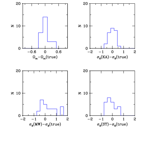
Figure 7: Histograms of the differences between the KL estimate of matter density, $\Omega_{m}$, and the linear normalization of the matter power spectrum, $\sigma_{8}$, with the input (true) values of the simulations. The biasing schemes are denoted by KA (high-peak biasing of Kaiser 1984), MW (Mo & White 1996) and ST (Sheth & Tormen 1998). The frequency distributions are obtained with 27 REFLEX-like subsamples selected from the Hubble Volume Simulation.

We selected 27 independent REFLEX-like subsamples from the LCDM Hubble Volume cluster sample. The average number of clusters per sample and its standard deviation is $435\pm 28$, similar to the 428 REFLEX clusters used for the final analyses. The redshift histograms closely resemble the observed distribution. We thus expect realistic error estimates from the simulations.

The histograms of the residuals between the values estimated with the KL method and the true (simulation input) values for $\Omega_{m}$ and for $\sigma_{8}$ as obtained with the three biasing models (see Sect. 3.2) are shown in Fig. 7.

The frequency distribution of the KL estimates of $\Omega_{m}$ gives the formal mean and standard deviation of $\Omega_{m}=0.32\pm 0.19$ (see Fig. 7, upper left). Note that the distribution is slightly skewed, the median value is $\Omega_{m}=0.27$. A $2\sigma$ clipping rejects two measurements and gives $\Omega_{m}=0.28\pm 0.14$. Whereas the mean value turns out to be quite stable, it appears to be more difficult to get a stable estimate of the error which includes cosmic variance. A still larger number of simulations is necessary to improve the accuracy. For the comparison with the internal errors given by the KL method (see Sect. 6) we use the latter more stable estimate, keeping in mind that the error could be underestimated by about 30%.

For the linear matter normalization the following formal means and standard deviations are obtained: $\sigma_{8}=0.87\pm 0.32$ (high-peak biasing, Fig. 7 upper right), $\sigma_{8}=1.20\pm 0.66$ (Mo & White biasing, Fig. 7 lower left), $0.82\pm 0.43$ (Sheth & Tormen biasing, Fig. 7 lower right). Note that for the computation of the means and standard deviations of the latter two biasing models only the values located in the high biasing regime are used (see Sect. 3.2.2). The errors include cosmic variance.

References

- [1] Bahcall, N.A., Fan, X., 1998, ApJ, 504, 1
- [2] Bond, J.R., 1995, Phys. Rev. Lett., 74, 4369
- [3] Borgani, S., Guzzo, L., 2001, Natur, 409, 39
- [4] Borgani, S., et al., 2001, ApJ, 561, 13
- [5] Böhringer, H., Guzzo, L., Collins, C.A., et al., 1998, The Messenger, 94, 21
- [6] Böhringer, H., Voges, W., Huchra, J.P., et al., 2000, ApJS, 129, 435
- [7] Böhringer, H., Schuecker, P., Guzzo, L., et al., 2001, A&A, 369, 826
- [8] Böhringer, H., Collins, C.A., Guzzo, L., et al., 2002, ApJ, 566, 93
- [9] Bryan, G.L., Norman, M.L., 1998, ApJ, 495, 80
- [10] Burles, S., Nollett, K.M., Turner, M.S., 2001, ApJL, 552, L1
- [11] Burles, S., Tytler, D., 1998, ApJ, 507, 732
- [12] Collins, C.A., Guzzo, L., Böhringer, H., et al., 2000, MNRAS, 319, 939
- [13] De Bernardis, P., Ade, P.A.R., Bock, J.J., et al. 2000, Nature, 404, 955
- [14] Einasto, J., Gramann, M., Saar, E., Targo, E., 1993, MNRAS, 260, 705
- [15] Einasto, J., Einasto, M., Gottlöber, S., et al., Nature, 385, 139
- [16] Eisenstein, D.J., Hu, W., 1998, ApJ, 496, 605
- [17] Evrard, A.E., MacFarland, T.J., Couchman, H.M.P., et al. 2001, astro-ph/0110246
- [18] Freedman, W.L., Madore, B.F., Gibson, B.K., et al. 2001, ApJ, 553, 47
- [19] Guzzo, L., Böhringer, H., Schuecker, P., et al., 1999, The Messenger, 95, 27
- [20] Haiman, Z., Mohr, J.J., Holder, G.P., 2001, ApJ, 553, 545
- [21] Jenkins, A., Frenk, C.S., White, S.D.M., Colberg, J.M., Cole, S., Evrard, A.E., Couchman, H.M.P., Yoshida, N., 2001, MNRAS, 321, 372
- [22] Jing. Y.P., Valdarnini, R., 1993, ApJ, 406, 6
- [23] Kaiser, N., 1984, ApJ, 284, L9
- [24] Karhunen, H., 1947, Ann. Acad. Science Finn. Ser. A.I. 37
- [25] Lahav, O., Bridle, S.L., Percival, W.J., et al., 2001, astro-ph/0112162
- [26] Loéve, M., 1948, Processes Stochastiques et Mouvement Brownien (Hermann: Paris)
- [27] Masi, S., Ade, P.A.R., Bock, J.J., et al., 2002, astro-ph/0201137
- [28] Matarrese, S., Coles, P., Lucchin, F., Moscardini, L., 1997, MNRAS, 286, 115
- [29] Mo, H.J., White, S.D.M., 1996, MNRAS, 282, 347
- [30] Moscardini, L., Matarrese, S., Lucchin, F., Rosati, P., 2000, MNRAS, 316, 283
- [31] Markevitch, M., 1998, ApJ, 504, 27
- [32] Matsubara, T., Szalay, A.S., Landy, S.D., 2000, ApJ, 535, L1
- [33] Miller, C.J., Batuski, D.J., 2001, ApJ, 551, 635
- [34] Peacock, J.A., West, M., 1992, MNRAS, 259, 494
- [35] Percival, W.J., Baught, C.M., Bland-Hawthorn, J., et al., 2001, MNRAS, 327, 1297
- [36] Press, W.H., Flannery, B.P., Teukolsky, S.A., Vetterling, W.T., 1989, Numerical Recipes (Cambridge Univ. Press, Cambridge)
- [37] Reiprich, T.H., Böhringer, H., 2002, ApJ, 567, 716
- [38] Retzlaff, J., 1999, PhD thesis, Univ. Potsdam
- [39] Retzlaff, J., Borgani, S., Gottlöber, S., Klypin, A., Müller, V., 1998, New Astron., 3, 631
- [40] Schuecker, P., Böhringer, H., Guzzo, L., et al., 2001, A&A, 368, 86
- [41] Seljak, U., Zaldarriaga, M., 1996, ApJ, 469, 437
- [42] Sheth, R.K., Tormen, G., 1999, MNRAS, 308, 119
- [43] Sugiyama, N., 1995, ApJS, 100, 281
- [44] Szalay, A., and the SDSS Collaboration, 2001, astro-ph/0107419
- [45] Tadros, H., Efstathiou, G., Dalton, G., 1998, MNRAS, 296, 995
- [46] Tegmark, M., Hamilton, A.J.S., Xu, Y., 2001, astro-ph/0111575
- [47] Trümper, J., 1993, Science, 260, 1769
- [48] Viana, P.T.P., Liddle, A.R., 1996, MNRAS, 281, 323
- [49] Voges, W., Aschenbach, B., Boller, Th., et al., 1999, A&A, 349, 389
- [50] Vogeley, M.S., Szalay, A., 1996, ApJ, 465, 34
- [51] Zandivarez, A., Abadi, M.G., Lambas, D.G., 2001, MNRAS, 326, 147