Period-doubling events in the light curve of R Cygni: evidence for chaotic behaviour

A detailed analysis of the century long visual light curve of the long-period Mira star R Cygni is presented and discussed. The data were collected from the publicly available databases of the AFOEV, the BAAVSS and the VSOLJ. The full light curve consists of 26655 individual points obtained between 1901 and 2001. The light curve and its periodicity were analysed with help of the $O-C$ diagram, Fourier analysis and time-frequency analysis. The results demonstrate the limitations of these linear methods. The next step was to investigate the possible presence of low-dimensional chaos in the light curve. For this, a smoothed and noise-filtered signal was created from the averaged data and with help of time delay embedding, we have tried to reconstruct the attractor of the system. The main result is that R Cygni shows such period-doubling events that can be interpreted as caused by a repetitive bifurcation of the chaotic attractor between a period $2T$ orbit and chaos. The switch between these two states occurs in a certain compact region of the phase space, where the light curve is characterized by $\sim$1500-days long transients. The Lyapunov spectrum was computed for various embedding parameters confirming the chaotic attractor, although the exponents suffer from quite high uncertainty because of the applied approximation. Finally, the light curve is compared with a simple one zone model generated by a third-order differential equation which exhibits well-expressed period-doubling bifurcation. The strong resemblance is another argument for chaotic behaviour. Further studies should address the problem of global flow reconstruction, including the determination of the accurate Lyapunov exponents and dimension.

1 Introduction

Red giants on the Asymptotic Giant Branch (AGB) of the Hertzsprung-Russell diagram are pulsationally unstable and show characteristic light variations. The traditional classification (Kholopov et al. 1985–88) is based on two properties of the visual light curve, the periodicity and full amplitude. Monoperiodic stars with amplitudes larger than 2$\aas@@fstack{m}$5 are the Mira-type variables, smaller amplitude or complex light curves place a star among the semiregular variables. Even the monoperiodic Mira stars do not have strictly repeating light variations, as there are apparently irregular cycle-to-cycle changes in amplitude and/or period. The overwhelming majority of related studies addressed the problem of period change, from the early works of Eddington & Plakidis (1929), Sterne & Campbell (1936) to more recent studies of Isles & Saw (1987), Lloyd (1989), Percy & Colivas (1999) and long series of papers by Koen & Lombard (from Koen & Lombard 1993 to Koen & Lombard 2001). Besides a few detections of significant gradual period change (e.g. Gál & Szatmáry 1995, Sterken et al. 1999), most of the studies concluded that random period fluctuations dominate the Mira light curves. Interestingly, the amplitude variations remained quite unstudied, likely because of the nature of the only existing data – low precision visual observations. Very few investigations can be found on this issue, the most important ones include an analysis of observations by Canizzo et al. (1990) and a theoretical study by Icke et al. (1992). Both papers inspected the possible presence of chaos in long-period variables. While Canizzo et al. (1990) rejected the hypothetic low-dimensional chaos in the three stars studied, Icke et al. (1992) argued that there is a lot of evidence for chaotic behaviour in the red giant variations.

Variable stars are primary targets of nonlinear analyses attempting to detect low-dimensional chaos in astrophysical systems. The most successful detections are associated with pulsating white dwarfs (e.g. Goupil et al. 1988, Vauclair et al. 1989), W Vir model pulsations (Buchler & Kovács 1987, Serre et al. 1996b) and two RV Tauri type stars, R Sct (Kolláth et al. 1990, Buchler et al. 1996) and AC Her (Kolláth et al. 1998). A common feature is the period-doubling bifurcation, which occurs in many simplified model oscillators, too (e.g. Saitou et al. 1989, Seya et al. 1990, Moskalik & Buchler 1990). Most recently, Buchler et al. (2001) presented an overview of observational examples of low-dimensional chaos including the first preliminary results for four semiregular stars (SX Her, R UMi, RS Cyg and V CVn). The emerging view of irregular pulsations is such that large luminosity-to-mass ratio strongly enhances the coupling between the heat flow and the acoustic oscillation. Consequently, the relative growth rates for relevant pulsation modes are of order of unity which is the necessary condition for chaotic behaviour. Since it is naturally satisfied in the low-mass, high-luminosity AGB stars, they are likely candidates for chaotic pulsations.

In this study, we analyse the visual light curve of the Mira star R Cygni (= HD 185456 = IRAS 19354+5005, spectral type S6/6e with Tc-lines, Jorissen et al. 1998). It is a bright, well-observed variable star with an average period of $\sim$430 days and average light extrema at $\sim$7$\aas@@fstack{m}$0 and $\sim$14$\aas@@fstack{m}$0. The light variation was discovered by Pogson in 1852 and the available magnitude estimates date back to the late 19th century. It has been studied by numerous authors (the ADS lists 179 references), mostly spectroscopically. Wallerstein et al. (1985) pointed out the correlation between brightness at maximum and interval from the previous cycle (fainter maxima occur later than normal). R Cyg was also included in a sample of 355 long period variables studied by Mennessier et al. (1997) who presented a classification of the light curves of LPVs for a discrimination between carbon- and oxygen-rich stars. To our knowledge, there is no further study dealing with the light variation of this star.

The main aim of this paper is to present a thorough analysis of the hundred-years long light curve. The paper is organised as follows. The observations and data preparation are described in Sect. 2. An intention to interpret the light curve with standard linear methods is discussed in Sect. 3. The nonlinear analysis is presented in Sect. 4, while concluding remarks and further directions are listed in Sect. 5.

2 Observations and data preparation

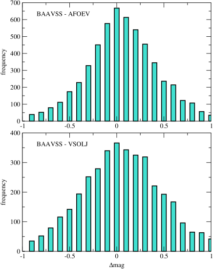
Figure 1: The distribution of the magnitude differences computed for 10-day means of the BAAVSS and AFOEV data (top) and the BAAVSS and AFOEV data (bottom). The maxima at 0 indicate good agreement between the different data.

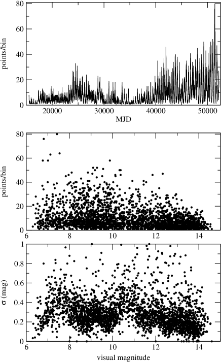
Figure 2: Top panel: The evolution of number of points per bin along the light curve. Middle panel: The same parameter against the apparent magnitude. Note the slightly triangular distribution with more data in the brighter states. Bottom panel: The mean deviation of estimates from the mean values (denoted with $\sigma$).

Table 1: A summary of the analysed datasets (MJD=JD$-$2400000).

Source	MJD(start)	MJD(end)	No. of points
AFOEV	22805	52181	8835
BAAVSS	15513a	51907	11024
VSOLJ	22597	51539	5888
VSNET	49718	52237	1105
Total:	15513	52237	26852
Corrected:	15513	52237	26655

^a 8 points between MJD 11737 and 13411 were excluded.

Data were taken from the databases of the following organizations: the Association Française des Observateurs d’Etoiles Variables (AFOEV), the British Astronomical Association, Variable Star Section (BAAVSS) and the Variable Star Observers’s League in Japan (VSOLJ). Since these data end in early 2001, the latest part of the light curve is covered with data obtained via the VSNET computer service.

The basic properties of the datasets are listed in Table 1. The three main sources are highly independent, as very few (less then 1%) duplicated and no triplicated data points were found. The total number of estimates (duplicates counted twice) is 26852. Before merging the data we have checked the data homogeneity with a simple statistical test. We have calculated 10-day means for all of the three major data sources (BAAVSS, AFOEV, VSOLJ) and compared their values in the overlapping regions. Since the British data are the longest one, we computed magnitude differences in sense of $\langle$BAAVSS$\rangle$ minus $\langle$AFOEV$\rangle$ and $\langle$BAAVSS$\rangle$ minus $\langle$VSOLJ$\rangle$. Their distribution is plotted in Fig. 1. While the AFOEV data result in a quite symmetric distribution, there is a suggestion for the VSOLJ data for being slightly brighter in average than the BAAVSS data. However, the highest peak at $\Delta$mag=0 and the symmetric nature for both distributions suggest that there is no need to shift any of the data and thus, we simply merged all data. After merging the original data files, we checked the deviant points by a close visual inspection of the combined light curve. Almost 200 points were rejected and the finally adopted set contains 26655 visual magnitude estimates.

The first step in the data processing was averaging the light curve using ten-day bins. With the binning procedure some statistical findings were revealed. First, we plotted the number of points per bin against time (Fig. 2, top panel). Here one can find fairly high number of points per bin (with steady increase in time) which is a necessary condition for calculating accurate mean values. Second, the distribution of the same parameter against the apparent magnitude (Fig. 2, middle panel) shows that there are typically 5–10 points per bin even in the faintest state, which is enough for good mean values. Finally, the mean deviation of the individual points against the apparent magnitude (Fig. 2, bottom panel) does not show significant trends, therefore, from a statistical point of view, the calculated mean light curve can be regarded quite homogeneous. The typical uncertainty of a single observation can be thus estimated as $\pm$0$\aas@@fstack{m}$5. Consequently, the uncertainty of the calculated mean values ($\approx\pm 0\aas@@fstack{m}5/\sqrt{N_{\rm obs}}$) ranges from $\pm$0$\aas@@fstack{m}$08 to $\pm$0$\aas@@fstack{m}$17. The binned light curve is presented in Fig. 3. The fact, that there are quite long subsegments, in which alternating maxima are obviuously present, reminded us of the case of RV Tauri type stars, i.e. pulsating yellow giants with alternating minima. This alternation in R Sct and AC Her was interpreted as being caused by low-dimensional chaos (Kolláth 1990, Kolláth et al. 1998) and that is why we tackled the question of possible chaotic behaviour in the light curve of R Cyg. The light curve shape also closely resembles that of some pulsating white dwarfs (e.g. Goupil et al. 1988), though with a characteristic time-scale of five order of magnitudes larger.

Since we intended to study the light variation with tools of the nonlinear time-series analysis, further preprocessing was done by smoothing and interpolating the binned light curve. First, we fitted Akima splines (Akima, 1970) to the binned data to get an equidistant series of light curve points, keeping the 10-day length (it means $\approx$43 points per cycle which is a fairly good sampling). The spline fit was further smoothed with a Gaussian weight-function, where we choose a wider (FWHM=20 days) Gaussian than in the case of studies of semiregular variables (Kiss et al. 1999, Lebzelter & Kiss 2001). We have experimented with various FWHMs starting from 5 days up to 30 days; the nonlinear analysis showed that much clearer images of the attractor can be reached if the observational noise, as well as remaining noise that is extraneous to the star (e.g. high-frequency components due to low-amplitude, but high-dimensional jitter, see Buchler et al. 1996) is smoothed out. The adopted 20 days provided well-smoothed signal with no zig-zags in the light curve and avoided strong amplitude decrease due to oversmoothing as in the case of FWHM=30 days. The final result is a dataset {$s(t_{\rm n})$} that is sampled at constant 10 days intervals. In Fig. 4 we show some typical observed light curve segments with the smoothed and noise-filtered signal. Obviously, some sharp features are missed in the latter data, however, as will be presented later, the success of our nonlinear analysis supports our data processing. In order to enable for the reader to study this interesting star with other nonlinear methods, we make the original 10-day means and the smoothed and noise-filtered data publicly available in electronic form at CDS, Strasbourg

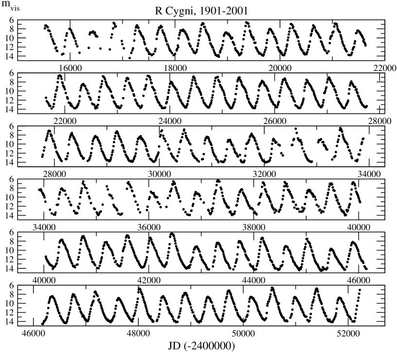
Figure 3: The whole dataset of R Cygni (10-day means). Note the presence of alternating maxima, especially in the lowest two panels.

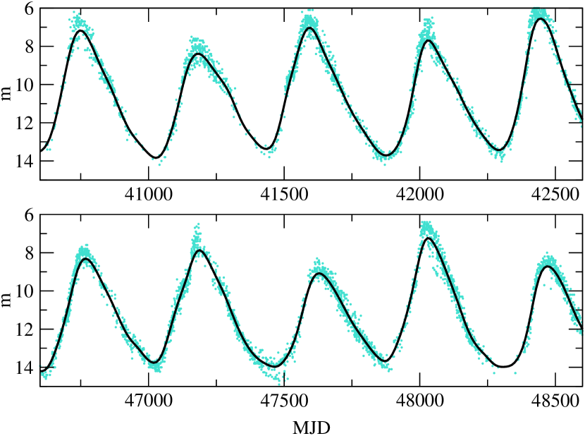
Figure 4: Typical observed light curve segments (light dots) with the smoothed and noise-filtered signal (solid line).

3 Standard methods

In this Section the period variation is examined with the $O-C$ diagram and one of its descendants, then we show that Fourier-analysis fails to give a full description of the light curve. Furthermore, fairly strong subharmonic components occur in the frequency spectrum which will be naturally included in the adopted nonlinear description discussed in the next Section. Two time-frequency methods are used to draw some constraints on the stability of the frequency content.

3.1 Period change

Traditional variable star research studying single-periodic light variations strongly relies on the $O-C$ method, although it has been shown in many cases that Mira stars usually do not fit the requirements of its application. This is due to the large intrinsic period fluctuations found in these variables (see, e.g. recent studies by Sterken et al. 1999, Percy & Colivas 1999), but even white noise (Koen 1992) or low-dimensional chaotic systems (Buchler & Kolláth 2001) can generate curved $O-C$ diagrams leading to spurious detections of long-term period changes. Nevertheless, despite the many possible interpretations, it might be interesting to show the results of this traditional method.

In order to construct the $O-C$ diagram we have determined all times of maxima from the binned light curve shown in Fig. 3. This was done by fitting low-order (3–5) polynomials to the selected parts of the light curves around maxima. Typically, we selected $\pm$60–70 days around a given maximum (this means $\sim$13–15 points of the light curve) and fitted polynomials with different orders chosen to give optimal fit (as judged by a visual inspection of the data). The fitted interval slightly changed with time as several cycles were covered only partially. Thanks to the extraordinarily good global light curve coverage, no cycle was lost between 1901 and 2001, thus we could determine 86 epochs of maximum. A mean period of 428 days given by the Fourier analysis of the whole dataset (next subsection) and the eighth epoch (MJD 18531) was used to construct the $O-C$ diagram plotted in Fig. 5.

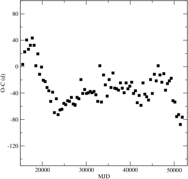
Figure 5: The $O-C$ diagram of R Cyg ($E_{0}$=MJD 18531, $P$=428 d). The typical uncertainty of a given point is about $\pm$10 days.

Three different “linear” segments appear in the $O-C$ diagram which could be explained by two period jumps at MJD 23500 and MJD 47200. However, little can be said about the astrophysical meaning of these jumps. Following the work by Percy & Colivas (1999), we performed the Eddington-Plakidis test (Eddington & Plakidis 1929) to estimate the amount of random period fluctuation $\epsilon$. The resulting relative fluctuation $\epsilon/P$ is 0.01 that places R Cygni close to the lower boundary of Fig. 2 in Percy & Colivas (1999), which means a relative stability of the mean period compared to other Mira stars of similar periods. Our most important conclusion here is that we can exclude the star to be undergoing noticeable long-term evolution (due to, e.g., a thermal pulse deep in the stellar interior, Wood & Zarro 1981) over the one century of observations. The apparent period is shorter at the very end of the dataset, but its variation does not seem to be a result of a slow period evolution. We note, that Koen & Lombard (2001) used simultaneously the epochs of maxima and minima to test for period changes in long-period variables which is a more effective approach than that of the $O-C$ diagram – at least in those cases, where only times of maxima and minima are available. In our case, the use of the full light curve is strongly favoured instead of examining any particular part of it.

3.2 Fourier analysis

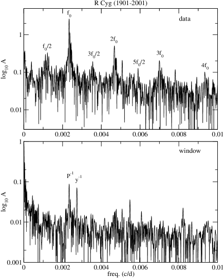
Figure 6: The frequency spectrum of R Cygni (top panel). Note the presence of subharmonic components up to 5/2 $f_{0}$. The window function shows two alias peaks, one is the 1-year alias due to seasonal gaps, while the other one at 0.00233 d^-1 (i.e. 1/430 d^-1) is caused by a few unobserved minima in the light curve.

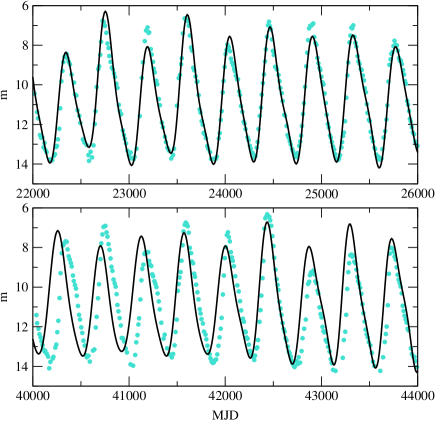
Figure 7: A comparison of the 15 frequency fit with the interpolated (top) and extrapolated (bottom) data (see text for details). The extrapolation obviously fails.

To investigate possible multiperiodicity, we have carried out a Fourier analysis with subsequent prewhitening steps. We have used Period98 of Sperl (1998) which also includes multifrequency least squares fitting of the parameters. The studied frequency range was 0–0.01 d^-1 with a step size of $1.8\cdot 10^{-6}$. We have also determined the main period in all 6 subsets plotted in Fig. 3 to compare apparent period change with the suggestions of the $O-C$ diagram.

The calculated amplitude spectrum of the whole light curve is presented in Fig. 6, where the window function is shown, too. The primary peak is at $f_{0}$=0.002338 d^-1 ($P=428$ d). The structure of the frequency spectrum is quite complex. One can find the integer harmonics of the main frequency (2$f_{0}$, 3$f_{0}$, 4$f_{0}$), while subharmonic components are present, too (3$f_{0}$/2, 5$f_{0}$/2). Note, that these subharmonic components are not introduced by the Fourier approach through subsequent prewhitening with sine curves, as Fig. 6 shows the frequency spectrum before any prewhitening. Their presence is due to the alternating amplitude changes; this has been proven by a very simple test. We have created artificial light curves by repeating i) a single cycle 50 times and ii) a double cycle with successive low and high amplitudes 25 times. Then the computed Fourier spectra clearly marked the reason for the subharmonics.

The main problem is that instead of well-determined narrow peaks, there are closely separated groups of peaks at the mentioned frequency values. The first 25 prewhitening steps resulted in 8 components in the range 0.002249–0.002464 d^-1 ($\approx f_{0}$), 4 components in the range 0.004605–0.004781 d^-1 ($\approx 2f_{0}$), 6 components in the range 0.001007–0.001437 d^-1 ($\approx f_{0}/2$), 1 component at 0.003558 ($\approx 3f_{0}/2$), 1 component at 0.007001 ($\approx 3f_{0}$) and 5 low-frequency components corresponding to the apparently irregular mean brightness variation. However, even the 25-frequency fit leaves a residual scatter of 0$\aas@@fstack{m}$52 being much larger than the expected uncertainty of the points. Therefore, the fit, besides being physically irrelevant, is still not perfect.

Another test of the multiperiodic hypothesis was done as follows. We have taken the first half of data, between MJD 15000 and 34000. This subset was Fourier analysed with the same procedure. The first 15 frequencies yielded an acceptable fit of the whole subset. Then this set of frequencies (and amplitudes and phases) was used to predict the second half of data. As expected, the extrapolation failed. This is demonstrated in Fig. 7, where subsets of the halves are plotted with the interpolating and extrapolating fits. The extrapolated signal has obviously lost its predictive power. Again, we have to reject the multiperiodic description of the light curve.

The frequency grouping found in R Cyg is exactly the same what as the one found for R Sct by Kolláth (1990) and AC Her by Kolláth et al. (1998). In those cases detailed tests showed that multiple periodicity can be excluded as the reason for the high number of components in the Fourier spectrum. Furthermore, such behaviour is characteristic for chaotic systems, e.g., the well-studied Rössler oscillator (see Serre et al. 1996a and Buchler & Kolláth 2001 for detailed discussions in astronomical terms).

The presence of subharmonic components is another interesting property. Similar subharmonics were found in a number of pulsating white dwarf stars in which they were interpreted as indications of period-doubling bifurcation (e.g. Vauclair et al. 1989). The $f_{0}$/2 subharmonic is usually accepted indicator of period-doublings. This subharmonic is fairly strong in the Rössler oscillator (see, e.g., Fig. 3 in Serre et al. 1996a) or other chaotic systems where pronounced period-doubling occurs (a closely related example is the case of W Vir hydrodynamic models analysed by Serre et al. 1996b).

The separate analysis of 6 segments, each being $\sim$6000 days long illustrates the essentially insignificant changes of the main period. The resulting periods are the following: MJD 15500–21600: 423$\pm$1.5 d; MJD 21600–27700: 429$\pm$2 d; MJD 27700–33900: 428$\pm$1 d; MJD 34000–40000: 428$\pm$0.5 d; MJD 40000–46100: 427$\pm$3.2 d; MJD 46100–52200: 422$\pm$1 d. This gives the same picture of the period change as the $O-C$ diagram does: slightly shorter periods at the beginning and end of the data, between them the mean period was constant. However, the given differences are consistent with the random fluctuations of the period at 1% level.

3.3 Time-frequency analysis

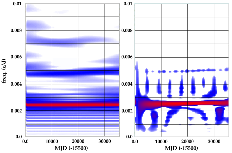
Figure 8: The wavelet map (left) and Choi-Williams distribution (right) for R Cyg.

Modulations and sudden changes of the light curve (i.e. time-dependent frequency content) can be studied with several time-frequency methods. In variable star research, one of the widely used methods is the wavelet analysis (Szatmáry et al. 1994 and references therein). A more efficient method is the use of of Choi-Williams distribution (CWD, Choi & Williams 1989) which enhances the sharp features in the time-frequency-amplitude space.

We present both the wavelet map and CWD in Fig. 8. They were calculated with the software package TIFRAN (TIme FRequency ANalysis) developed by Z. Kolláth and Z. Csubry at Konkoly Observatory, Budapest. As expected, the main ridge at $f\approx 0.0025$ d^-1 is the most obvious feature, while its harmonics are visible up to the third order. Subharmonic components can be identified in the CWD and we also noticed a slight tilt of the ridges (most emphasized for $2f_{0}$) in the last third of the data. The suggested period shortening around MJD 40000 (note the $-$15500 shift of the horizontal axes in Fig. 8) is in good agreement with the results of the Fourier analysis. Unfortunately, little can be inferred about the physical system behind the light variation. Time-frequency analysis, similarly to Fourier analysis, is basically an interpolation method. There are strict limitations and real understanding needs a completely different approach. This is provided by the methods of nonlinear time-series analysis.

4 Nonlinear analysis

During the last two decades, there has been a growing interest in nonlinear studies of variable stars. Several examples of seemingly irregular light curves were interpreted as results of low-dimensional chaotic behaviour. Buchler and his co-workers published some fundamental papers dealing with either theoretical interpretations or analyses of observations. There has been a number of excellent papers and reviews in the astronomical literature on this topic (e.g. Perdang 1985, Serre et al. 1996a, Buchler et al. 1996, Buchler & Kolláth 2001), where the reader can find definitions and descriptions of the analysing methods.

Hereafter we assume that the light curve is generated by a deterministic dynamical sytem of a physical dimension $d$. In this section, we employ various techniques to unfold the multidimensional structure of this system in reconstructed phase spaces. The most important method is the time delay embedding. We discuss some properties of the embedding and the reconstructed attractor of the system, based on the smoothed and noise-filtered light curve signal $\{s(t_{\rm n})\}$. For this purpose, we have extensively used the TISEAN package of Hegger et al. (1999), which is a publicly available software package consisting of practical implementations of nonlinear time-series methods. In the following we will refer to some routines of this package (e.g. mutual, false_nearest, svd etc.). Their use and basics are very well documented at the cited website.

4.1 Embedding parameters

The first issue is the optimal choice of embedding parameters. As has been discussed in, e.g., Buchler et al. (1996) different time delays ($\Delta$) and/or embedding dimension ($d_{\rm e}$) may result in completely different phase space reconstructions. In the case of R Sct and AC Her, a small range of fraction of the formal period (5–20%) yielded “optimal” results. We applied the routine mutual which calculates the time delayed mutual information suggested by Fraser & Swinney (1986) as a tool to determine a reasonable delay. The first minimum of the mutual information occured at $\Delta$=13 (note, that henceforth we normalize $\Delta$ with the 10-days long sampling rate) and a visual inspection of delay representations supported the optimal $\Delta$ to be between 10 and 15. The minimal embedding dimension was estimated by the false nearest neighbour method proposed by Kennel et al. (1992). False neighbours in the phase space occur when the reconstruction is done with a $d_{\rm e}<d$ and points well-separated in higher dimensions get closer due to projections into a lower dimension space. The idea is to find that dimension in which the embedding results in marginal amount of false neighbours, i.e. a “good” distribution of points is reached in the reconstructed phase space. The routine false_nearest calculates the fraction of false neighbours while changing $d_{\rm e}$ for a given distance threshold. The results of this method should be handled carefully, because in case of short datasets, it may underestimate the optimal dimension. For short sets and higher dimensions one gets few neighbours simply because the points sparsely occupy the embedding space. In our case $d_{\rm e}$=3 or 4 is suggested by this method, as the fraction of false neighbours decreases drastically for larger embedding dimensions (even for 5 and 6). Therefore, we adopted 10 to 15 as the reasonable range for $\Delta$ and 3, 4 for $d_{\rm e}$.

4.2 Recurrence plots

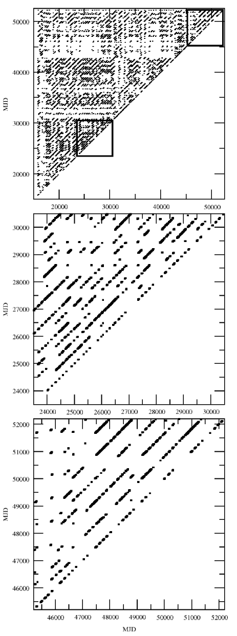
Figure 9: The recurrence plot and two subregions with different behaviour (marked with thick boxes in top panel).

To identify time resolved structures of the dataset, we have determined recurrence plots with various parameters (with the routine recurr). It is a very simple tool: it scans the time series and marks each pair of time indices $(i,j)$ whose corresponding delay vectors has distance $\leq\epsilon$ for a given $\epsilon$. Therefore, a black dot in the $(i,j)$-plane means closeness. If a periodic signal is examined, then the points tend to occur both on the diagonal and parallel lines separated from the main diagonal by integer multiplets of the period. These plots can be very well used to detect and confine transients in a dataset. Fortunately, the recurrence plot is not particularly sensitive to the choice of embedding parameters and we found only marginal, almost invisible differences when choosing embedding dimension and time delay within reasonable ranges (3–4 for $d_{\rm e}$ and 10–15 for $\Delta$). We show the recurrence plot of our data for $d_{\rm e}=3$ and $\Delta=13$ in (top panel in Fig. 9), whose values were chosen without any special consideration. In this Figure we have converted $(i,j)$ indices to MJD.

Several interesting conclusions can be drawn even from this very simple plot. A few well determined transients occured between MJD 16300–17300, 30700–32500 and 42700–46300 (with a certain ambiguity of the boundaries). The first one is probably caused by the lack of observations and thus uncertain spline interpolation, but the other two are real as they are well covered by data. Thus one has to be careful when analysing subsets that include the transient regions. The periodicity is obvious from the dense paralel lines in the plot. One can find large islands where the distance between the parallel lines jumps to the doubled period. To emphasize such details, we plot two subregions in the middle and bottom panels of Fig. 9. The latter one clearly corresponds to period-doubled region. By a close inspection of the top panel, one can find similarly period-doubled regions, e.g., around (20000,23000), (23000,41000) or (41000,41000) in $\sim 1500\times 1500$ wide blocks. Furthermore, it is interesting that both two large transients were similar as suggested by the clustered points around (30000,45000). It follows that the transients must have occured around a particular small region in the phase space, therefore, they were caused by the same process.

4.3 Visualization of the trajectories

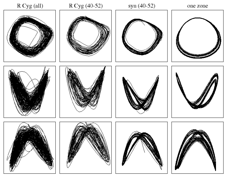
Figure 10: BK projections ($d_{\rm e}=4$, $\Delta=10$). See text for further detais.

To visualize the embedded state vectors $\mathbf{s}_{\rm n}$, we have generated the Broomhead-King (BK) projections (Broomhead & King 1986), which project onto the eigenvectors of the correlation matrix. In the TISEAN package, this can be done with the routine svd (i.e. singular value decomposition). We plot the most informative BK projections obtained from different data. The first column (R Cyg (all)) is based on the whole $\{s(t_{\rm n})\}$, with $d_{\rm e}=4$, $\Delta=10$. The second column (R Cyg (40–52)), with the same embedding parameters, contains the reconstructed attractor from the last third of the data, between MJD 40000 and 52200. Plots in the third column (syn (40–52)) are based on a synthetic dataset, which has been calculated by a locally linear prediction using the routine nstep. The determined local linear model can be iterated for an arbitrarily long time thus allowing the creation of synthetic datasets. In our case, the locally linear approximation was iterated for 2400 points (i.e. 24000 days). The reason for using only the last third of the data for the local linear model is the fact, that this way we only approximate the unknown map f of the system (Buchler & Kolláth 2001) with its local Taylor expansion. For longer data the linear model oversmooths the trajectories in the phase space thus blurring out the phase portrait of the attractor. The fourth column in Fig. 10 shows plots based on a simple one zone model discussed in the next section.

Our main conclusions are as follows. The embedding produces trajectories with remarkable structures. The global structure does not depend whether the whole set or some of its subsets are analysed. By iterating a locally linear approximation of the map we could get a cleaner image of the attractor which shows the period-doubling unambiguously. It is suggested that the system switches back and forth between a period $2T$ orbit and chaotic state. The switch occurs in a located region of the phase state and there shows the light curve its transients.

4.4 Lyapunov exponents and dimension, the correlation integral

The exponential growth of infinitesimal perturbations from which the chaos arises can be quantitatively characterized by the spectrum of Lyapunov exponents (e.g. Kantz & Schreiber, 1997 and references therein). If chaos is present in a dataset then one of the Lyapunov exponents should be positive. We estimated this maximal exponent by computing

$S(\epsilon,d_{\rm e},t)=\Bigg{\langle}{\rm ln}\Bigg{(}{1\over|\mathscr{U}_{\rm n}|}\sum\limits_{\mathbf{s}_{\rm n^{\prime}}\in\mathscr{U}_{\rm n}}|s_{\rm n+t}-s_{\rm n^{\prime}+t}|\Bigg{)}\Bigg{\rangle}_{\rm n}$

with the routine lyap_k ($\mathscr{U}_{\rm n}$ is the $\epsilon$-neighbourhood of $\mathbf{s}_{\rm n}$, excluding $\mathbf{s}_{\rm n}$ itself). If $S(\epsilon,d_{\rm e},t)$ shows a linear increase with the same slope for all $d_{\rm e}$ larger than some $d_{0}$ and for a range of $\epsilon$, then this slope is the estimate of the maximal exponent $\lambda_{1}$. We calculeted $S(\epsilon,d_{\rm e},t)$ using the whole $\{s(t_{\rm n})\}$ and plot the result in Fig. 11. Different branches corresponding to $d_{\rm e}$=3,4,5 and 6 and three values of $\epsilon$ show oscillations but are generally parallel. A global linear fit gives a slope 0.0244 corresponding to $\lambda_{1}$=0.00244 d^-1. This roughy equals to that of determined for R Sct ($\approx$0.0020 d^-1, Buchler et al. 1996) and smaller by a factor of 2–3 as for AC Her (Kolláth et al. 1998).

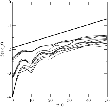
Figure 11: Estimating the maximal Lyapunov exponent. The solid line is the linear fit shifted vertically for clarity. The slope is 0.0244 implying $\lambda_{1}$=0.00244 d^-1.

The full Lyapunov spectrum was computed with the routine lyap_spec. Its results should be considered as only preliminary, because the method, similarly to nstep, employs local linear fits. It fits local Jacobians of the linearized dynamics and by multiplying them one by one to different vectors in tangent space, emerges the trajectories. The logarithms of rescaling factors are accumulated and their average give the Lyapunov exponents (Sano & Sawada 1985).

In order to give an indication of the robustness of the Lyapunov spectrum and Lyapunov dimension, we present their values for various embedding parameters in Table 2. In every cases, we find one positive exponent. Thus, the attractor is clearly chaotic. In most cases, the absolute value of the second exponent is smaller than the first by a factor of 3 to 5. An ideal flow should have $\lambda_{2}=0$ (Serre et al. 1996a), therefore our local fit is indeed only a rough approximation. Consequently, the determined Lyapunov dimensions scatter between 2 and 3 with no definite tendency. Unfortunately, as noted, e.g. in Serre et al. (1996a), the computation of all of the Lyapunov exponents requires very long datasets. This is the other reason why our results are fairly uncertain. A global nonlinear fit would yield results that are superior to ours presented here. We have to conclude that our methods do not allow an accurate determination and a further study should be devoted to i) a global flow reconstruction (Serre et al. 1996a) and ii) computation of more accurate Lyapunov exponents and dimension. The latter one is important because these numbers are the main quantitative parameters of a chaotic system.

Table 2: Lyapunov exponents (in 10^-4 d^-1) and dimension.

$d_{\rm e}$	$\Delta$	$\lambda_{1}$	$\lambda_{2}$	$\lambda_{3}$	$\lambda_{4}$	$\lambda_{5}$	$d_{\rm L}$
a)
3	15	17	$-$6	$-$57			2.19
4	8	27	$-$22	$-$38	$-$94		2.12
4	10	28	$-$9	$-$24	$-$114		2.81
4	15	19	$-$4	$-$19	$-$81		2.78
5	5	31	$-$30	$-$44	$-$72	$-$126	2.02
b)
3	15	26	$-$7	$-$67			2.30
4	8	38	$-$16	$-$45	$-$97		2.47
4	10	37	$-$11	$-$38	$-$89		2.70
5	5	30	$-$19	$-$35	$-$65	$-$182	2.30

$a)$ R Cyg (40–52)
$b)$ syn (40–52)

Finally, the correlation dimension was estimated by the correlation sum $C(d_{\rm e},\epsilon)$ (Grassberger & Procaccia 1983). This method was applied by Canizzo et al. (1990) for three long-period variable stars. In those cases, Canizzo et al. concluded that the light curves can be modelled with a regular and a stochastic component thus rejecting the hypothetic chaos. Buchler et al. (1996) argued against the use of correlation integral, claiming that typically available data are too short for this purpose. Nevertheless, we have computed the correlation sum to check its properties. For this, the routine c2naive was used which output was processed by the routine c2d. The latter routine computes ${\rm d}\log C(\epsilon)/{\rm d}\log\epsilon$ for which one expects a wide constant local minimum with different embedding dimensions (see detailed tests presented in Canizzo et al. 1990).

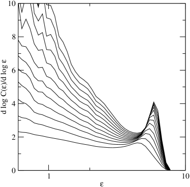
Figure 12: Correlation dimension estimation from the correlation sum. Embedding dimensions 3 to 25 are shown for odd numbers. Slopes are determined by straight line fits to the log-log plot of the correlation sum. Note that horizontal axis is logarithmic.

We show the results of our computations in Fig. 12. This diagram is based on the whole $\{s(t_{\rm n})\}$. Although we could not find the expected linear scaling region, the presented behaviour slightly resembles that of the Lorenz-attractor as shown in Canizzo et al. (1990) (see especially their Fig. 4b). The closely separated local minima suggest a fractal dimension between 2.0 and 2.3 for the attractor, though this estimate should be taken with caution. We conclude that the analysis of the correlation sum yields results that are compatible with the previous ones.

4.5 Comparison with a one zone model

We compare the presented behaviour of R Cygni with a simple one zone model with stressed period-doubling bifurcation. The similarity is provided by the reconstructed attractor. Although it has only marginal physical implications, the resemblance is quite illustrative.

As a simple model for the dynamic of a pulsating white dwarf star, Goupil et al. (1988) used the following third order differential equation

$x^{\prime\prime\prime}+Kx^{\prime\prime}+x^{\prime}+K\mu x(1+\beta x)=0$              (1)

corresponding to a one zone model that is analogous to Baker’s one zone model (Baker 1966). Here $x$ is the radial displacement from equilibrium. The control parameter is $\mu$, while $K=0.5$ and $\beta=-0.5$ was fixed (see Goupil et al. 1988 for their meaning). When $\mu$ is varied, the system first bifurcates from its stable fixed point to a stable limit cycle (period $T$ orbit at $\mu=-1$), while at $\mu=-1.66$ the first period-doubling bifurcation occurs. The period $T$ orbit becomes mildly unstable and a stable period $2T$ orbit exists. This was the main point which reminded us to the case of R Cygni and that is why we have solved Eq. (1) numerically. During the fourth order Runge-Kutta numerical integration we have added simple random perturbation that mimicked internal perturbations of the system. To allow an easy comparison with R Cygni, we have rescaled the time to get 430 days for the period of the one zone model.

The solution is compared with the light curve and its iterated locally linear approximation in Fig. 13. The amplitude does not change as much as in the original data, which is simply due to the fact, that Eq. (1) gives the variations of the radius, not the luminosity. There is, of course, some functional dependence between them, which is not expected to change the very basic nature of the reconstructed attractor. The calculated maximum alternation, its disappearance and reappearance is similar to what characterizes R Cygni, as has already been stressed by the BK projections. A further support is given by the Fourier spectra of data shown in Fig. 14. As discussed in Goupil et al. (1988), depending on how long and at what time we observe the system, we see an oscillation whose trajectory in phase space lies either on the period $2T$ orbit or on the period $T$ orbit (then disappears the $f_{0}/2$ subharmonic), or a mixed trajectory is observed switching over from one attractor to the other. In this case, the temporal behaviour exhibits a change in the alternation of small and large maxima. This largely reminds us of the light curve behaviour of R Cyg.

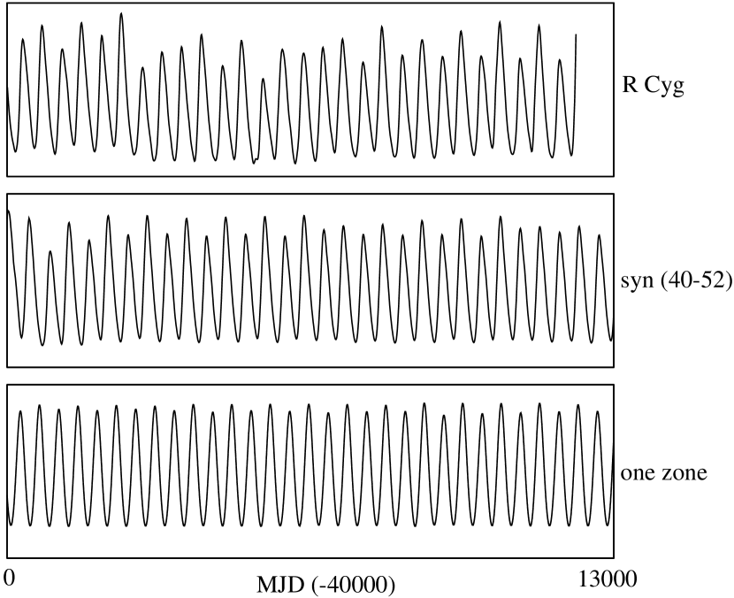
Figure 13: A comparison of R Cyg (40–52), syn (40–52) sets with the one zone model.

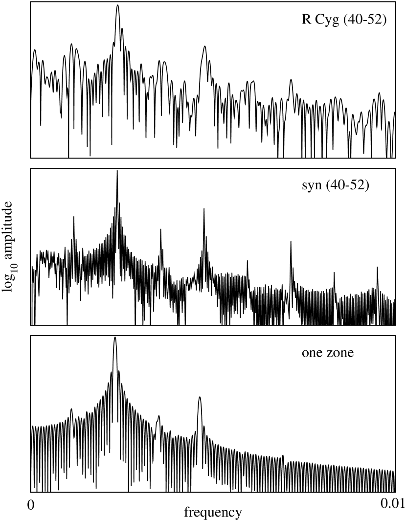
Figure 14: Fourier spectra of the data plotted in Fig. 13.

5 Conclusions

Our study concentrated on the demonstration of the low-dimensional chaotic behaviour in the light curve of a Mira star. For this, various linear and nonlinear methods has been applied. While the $O-C$ diagram is compatible with either stochastic (high dimensional random process) or chaotic (low-dimensional deterministic) dynamics, the frequency and time-frequency analyses raised the possibility of underlying chaos through the presence of subharmonic components. The strongest pieces of evidence came from the nonlinear analysis. Time delay embedding and different analyses of embedded state vectors in the reconstructed phase space revealed the following results:

1. The phase portraits show remarkably regular structures. The regularity does not depend whether the full dataset or some subsets are used for embedding. The estimated minimum embedding dimension was 3 or 4 as suggested the false nearest neighbours test. Other extensively used numerical methods favoured 4.

2. The long term behaviour is dominated with apparent period-doubling events. It can be interpreted as caused by a chaotic system which switches back and forth between a period $2T$ orbit and chaotic state. The switch occurs in a compact region of the phase space in which the light curve exhibits 1000–1500-days long transients.

3. The Broomhead-King projections were used to visualize the phase portraits. Synthetic data were generated with a locally linear fit to the attractor. They gave the clearest phase portraits showing unambiguously the period-doubling bifurcation.

4. Quantitative parameters, such as the Lyapunov exponents and dimension, were estimated, though with fairly large uncertainty. The estimated largest Lyapunov exponent is +0.0024 d^-1. This means that the distances between the neighbouring trajectories increase by $e$ during 417 days, i.e. we cannot predict the variation for longer time than one pulsation period. The Lyapunov spectrum was computed with the locally linear approximation with various embedding parameters. In every cases we found one positive exponent. In most case, the second one is close to 0 which is characteristic for ideal flows. The correlation sum, though rather inconclusively, suggests a fractal dimension 2.0–2.3 for the attractor.

5. We have compared the analysed data with a simple one zone model generated by a third-order differential equation. It shows such period-doubling bifurcation which is very similar to what is observed for R Cyg. The similarity of these two systems is our last argument for low-dimensional chaos in the light curve of R Cyg.

How can we compare our results with recent theoretical advancements in this field of variable star research? Most importantly, presence of low-dimensional chaos in a Mira star has been detected for the first time. This means that despite the complex structure of an AGB star, the pulsations in R Cyg occur in a very dimension reduced phase space. Presently, we cannot draw firm conclusions on the physical dimension of the system but our results suggest 3 or 4. In the latter case, a similar consideration might be applicable as for R Sct by Buchler et al. (1996). In that case, they concluded that the pulsations are the result of the nonlinear interaction of two vibrationally normal modes of the star. As soon as more sophisticated nonlinear methods are used to analyse the light curve of R Cyg, we will be able to infer more physical implications on the nature of pulsations. A further study will be devoted to a nonlinear global flow reconstrucion which enables, e.g. computing accurate Lyapunov spectrum and dimension. Only then it will be possible pinpointing the effective (physical) dimension of the phase space.

The examination of publicly available databases (AFOEV, VSOLJ, BAAVSS) revealed that there are at least a few dozen or even more than one hundred Mira stars with continuous, densely sampled visual light curves. R Cygni is only one of them. We list some Mira stars of similar period (400–470 days) with well-sampled light curves: T Cas, R And, R Lep, R Aur, U Her, $\chi$ Cyg, U Cyg, V Cyg, S Cep, RZ Peg, R Cas and Y Cas. A quick look at their AFOEV and VSOLJ data reveals a few examples with interesting light curves resembling that of R Cyg. Another further task is to spot those stars which might be twins of R Cyg and make an intercomparison between them. It is expected that the discovery of other similar stars may help to extend the observational base of a new discipline, the nonlinear asteroseismology (Buchler et al. 1996) which extracts quantitative information from the irregular light curves. It is, of course, still in its infancy and more theoretical as well as observational efforts have to be undertaken.

- (1) Akima, H. 1970, Journal of ACM, 17, 589
- (2) Baker, N. 1966, In: Stellar Evolution, Eds. R. F. Stein & A. G. W. Cameron, New York: Plenum Press, p. 333
- (3) Broomhead, D. S., & King, G. P. 1986, Physica D, 20, 217
- (4) Buchler, J. R., & Kovács, G. 1987, ApJL, 320, L57
- (5) Buchler, J. R., & Kolláth, Z. 2001, In: Stellar pulsation - nonlinear studies, Eds.: M. Takeuti & D. D. Sasselov, ASSL, Vol. 257, Dordrecht: Kluwer Academic Publishers, p. 185 (astro-ph/0003341)
- (6) Buchler, J. R., Kolláth, Z., Serre, T., & Mattei, J. 1996, ApJ, 462, 489
- (7) Buchler, J. R., Kolláth, Z., & Cadmus, R.R., Jr. 2001, In: Proc. “Experimental Chaos 2001”, The 6th Experimenal Chaos Conference, Potsdam, Germany, in press (astro-ph/0106329)
- (8) Canizzo, J. K., Goodings, D. A., & Mattei, J. A. 1990, ApJ, 357, 235
- (9) Choi, H. I., & Williams, W. J. 1989, IEEE Trans. Acoust., Speech, Signal Proc., 37, 862
- (10) Eddington, A. S., & Plakidis, L. 1929, MNRAS, 90, 65
- (11) Fraser, A. M., & Swinney, H. L. 1986, Phys. Rev. A, 33, 1134
- (12) Gál, J., & Szatmáry, K. 1995, A&A, 297, 461
- (13) Goupil, M. J., Auvergne, M., & Baglin, A. 1988, A&A, 196, L13
- (14) Grassberger, P., & Procaccia, I., 1983, Physica D, 9, 189
- (15) Hegger, R., Kantz, H., & Schreiber, T. 1999, Chaos, 9, 413 (chao-dyn/9810005)
- (16) Icke, V., Frank, A., & Heske, A. 1992, A&A, 258, 341
- (17) Isles, J. E., & Saw, D. R. B. 1987, JBAA, 97, 106
- (18) Jorissen, A., Van Eck, S., Mayor, M., & Udry, S. 1998, A&A, 332, 877
- (19) Kantz, H., & Schreiber, T. 1997, Nonlinear Time Series Analysis, Cambridge University Press, Cambridge
- (20) Kennel, M. B., Brown, R., & Abarbanel, H. D. I. 1992, Phys. Rev. A, 45, 3403
- 1985– (88) Kholopov, P. N., Samus, N. N., Frolov, M. S., et al., 1985–88, General Catalogue of Variable Stars, edition, “Nauka” Publishing House, Moscow (GVCS)
- (22) Kiss, L. L., Szatmáry, K., Cadmus, R. R., Jr., & Mattei, J. A. 1999, A&A, 346, 542
- (23) Koen, C. 1992, In: Variable Stars and Galaxies, ASP Conf. Series, 30, 127
- (24) Koen, C., & Lombard, F. 1993, MNRAS, 263, 287
- (25) Koen, C., & Lombard, F. 2001, MNRAS, 325, 1124
- (26) Kolláth, Z. 1990, MNRAS, 247, 377
- (27) Kolláth, Z., Buchler, J. R., Serre, T., & Mattei, J. 1998, A&A, 329, 147
- (28) Lebzelter, T., & Kiss, L. L. 2001, A&A, 380, 388
- (29) Lloyd, C. 1989, Observatory, 109, 146
- (30) Mennessier, M. O., Boughaleb, H., & Mattei, J. A. 1997, A&AS, 124, 143
- (31) Moskalik, P., & Buchler, J. R. 1990, 355, 590
- (32) Percy, J. R., & Colivas, T. 1999, PASP, 111, 94
- (33) Perdang, J. M. 1985, In: Chaos in Astrophysics, Eds. J. R. Buchler, J. M. Perdang & E. A. Spiegel, Dordrecht: D. Reidel Publishing Company, p. 11
- (34) Saitou, M., Takeuti, M., & Tanaka, Y. 1989, PASJ, 41, 297
- (35) Sano, M., & Sawada, Y. 1985, Phys. Rev. Lett., 55, 1082
- (36) Serre, T., Kolláth, Z., & Buchler, J.R. 1996a, A&A, 311, 833
- (37) Serre, T., Kolláth, Z., & Buchler, J.R. 1996b, A&A, 311, 845
- (38) Seya, K., Tanaka, Y., & Takeuti, M. 1990, PASJ, 42, 405
- (39) Sperl, M. 1998, Comm. Astr. Seis. 111
- (40) Sterken, C., Broens, E., & Koen, C. 1999, A&A, 342, 167
- (41) Sterne, T. E., & Campbell, L. 1936, Harvard Ann., 105, 459
- (42) Szatmáry, K., Vinkó, J., & Gál, J. 1994, A&AS, 108, 377
- (43) Vauclair, G., Goupil, M.J., Baglin, A., et al. 1989, A&A, 215, L17
- (44) Wallerstein, G., Hinkle, K. H., Dominy, J. F., et al. 1985, MNRAS, 215, 67
- (45) Wood, P.R., & Zarro, D.M., 1981, ApJ, 247, 247