LAMBDA-INFLATION VERSUS OBSERVATIONS

Lambda-inflation is tested against CMB and LSS observational data. The constraints for inflationary parameters are considered.

1 Introduction

An increasing precision of measurements in observational cosmology requires the adequate accuracy of predictions in the early Universe theory. It is particularly true for numerious recent and on-going experiments to measure the CMB angular anisotropy (BOOMERanG $\!{}^{{\bf?}}$, MAXIMA $\!{}^{{\bf?}}$, DASI $\!{}^{{\bf?}}$, VSA $\!{}^{{\bf?}}$, CBI $\!{}^{{\bf?}}$, ARCHEOPS, MAP).

The inflationary paradigm is still the only viable theory of the early Universe. There is no doubt that inflation explains the observable features of the Universe much better than other theories (for example, string or ekpyrotic ones). One of such features is well established flattness of the Universe $\!{}^{{\bf?},{\bf?},{\bf?},{\bf?}}$. Other important predictions of inflation is related to the production of cosmological perturbations. If the potential of inflaton is determined, the spectra of scalar and tensor perturbations can be derived by means of any of existing formalisms. Here I use the historically first one proposed in $\!{}^{{\bf?}}$.

A majority of papers dedicated to the numerical analysis of cosmological models considers scale-free cosmological perturbation spectra whereas almost all inflationary models predict more complicated forms of them. In addition, in many inflationary models the cosmic gravitational waves significantly contribute into the large scale CMB anisotropy and have to be taken into account.

This problem may be solved in two ways. The first is testing given inflationary models. This way requires accurate calculations of scalar and tensor perturbation spectra. The precision of such method is related with the validity of slow-rolling approximation. The second way is phenomenological one. It is based on the assumption that a density perturbation spectrum can be approximated by power law, $k^{n}$, where $n$ may be constant or slowly depending on scale. In the latter case a new parameter, the running $\partial n/\partial\ln k$, appears (see, e.g., $\!{}^{{\bf?}}$ and references wherein).

My present analysis is related with the first way.

2 Lambda-inflation

I call by Lambda-inflation a model with a single scalar field $\varphi$ and the following inflaton potential:

$$V(\varphi)=V_{0}+\frac{1}{\kappa}\lambda_{\kappa}\varphi^{\kappa},$$ (1)

where $V_{0}$, $\lambda_{\kappa}$, $\kappa$ are constants (see also $\!{}^{{\bf?},{\bf?}}$). I will concentrate on a model with $\kappa=4$.

This model is often referred in literature as “hybrid inflation” $\!{}^{{\bf?}}$. I reserve the latter name for the case of Lambda-inflation, where some particular way of the decay of the effective Lambda-term ($V_{0}$) is assumed.

It is convinient to introduce two new parameters. The first of them, $c$, is as follows:

$$c\equiv\frac{1}{2}\sqrt{\frac{V_{0}}{\lambda}}$$ (2)

(here and below $\lambda\equiv\lambda_{\kappa}$). $c$ is closely related to the critical field value where both terms of the potential are equal to each other ($\varphi_{cr}=2\sqrt{c}$). The second parameter, $k_{cr}$, is a scale when $\varphi$ reaches $\varphi_{cr}$. The slow-roll approximation is valid for $c\gg 1$. In this case the spectra of perturbations are as follows:

$${\rm S}:\;\;\;\;\;q_{k}=\frac{H}{2\pi\sqrt{2\gamma}}=\frac{\sqrt{2\lambda/3}}{\pi}\left(c^{2}+x^{2}\right)^{3/4},$$ (3)

$${\rm T}:\;\;\;\;\;h_{k}=\frac{H}{\pi\sqrt{2}}=\frac{2c\sqrt{\lambda/3}}{\pi}\left(1+\frac{x}{\sqrt{c^{2}+x^{2}}}\right)^{-1/2},$$ (4)

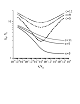
where $H$ is the Hubble constant, $\gamma\equiv-\dot{H}/H^{2}$, $x\simeq\ln\left(k/k_{cr}\right)$ (see details in $\!{}^{{\bf?},{\bf?}}$). Figure 1 illustrates these formulas.

Figure 1: Scalar ($q_{k}$, dash lines) and tensor ($h_{k}$, solid lines) perturbation spectra in Lambda-inflation (arbitrary normalization).

3 Cosmological model

Cosmological parameters can be separated into few groups. One of them contains inflationary parameters describing spectra of the cosmological perturbations (usually, they are the slopes, $n_{S}$, $n_{T}$, and amplitudes, $q_{k}$, $h_{k}$). Another set of parameters describes matter and energy in the Universe (the matter density parameter, $\Omega_{m}$, $\Lambda$-term, $\Omega_{\Lambda}$, the baryon abundance, $\Omega_{b}$, the massive neutrino abundance, $\Omega_{\nu}$, the number of massive neutrino species $N_{\nu}$, etc.). Another important cosmological parameter is the value of Hubble constant, $H_{0}=100h\;{\rm km}\;{\rm s}^{-1}{\rm Mpc}^{-1}$. This short list of cosmological parameters may be expanded.

The complete analysis of complex cosmological model is a very hard task: one has to use both a large number of free parameters and all available experimental data related to the determination of cosmological model ($\Delta T/T$, cluster abundance data, $Ly_{\alpha}$ data, and others).

Let us simplify this task. Firstly, let us fix values of the cosmological parameters describing dark matter and energy. Here I assume $\Omega_{\Lambda}=0.65$, $\Omega_{c}=0.29$, $\Omega_{b}=0.05$, $\Omega_{\nu}=0.01$, $N_{\nu}=3$, $h=0.65$. Secondly, let us take only two observational tests, namely, COBE measurent of $\Delta T/T$ which determines the amplitude of $\Delta T/T$ at 10th spherical harmonic ($C_{10}$), and $\sigma_{8}$ which normalizes the spectrum of density perturbations.

As for $C_{10}$, we have some gravitational wave contribution coming from inflation. It is standardly described by T/S parameter: T/S$\equiv C^{\rm T}_{10}/C^{\rm S}_{10}$. The characterictic scale of COBE is $k_{COBE}\equiv k_{1}\simeq 1.5\times 10^{-3}h\;{\rm Mpc}^{-1}$. As for $\sigma_{8}$, the characteristic scale is $k_{\sigma_{8}}\equiv k_{2}\simeq 1.5\times 10^{-1}h\;{\rm Mpc}^{-1}\simeq 100k_{1}$.

After simple calculations we derive the following equation:

$$\left(1+{\rm T/S}\right)\left(\frac{q_{k_{1}}}{q_{k_{2}}}\right)^{2}=1,$$ (5)

The numerical solution of this equation can be approximated by linear fit:

$$\ln\frac{k_{1}}{k_{cr}}=0.32\,c-1.92,$$ (6)

the error is in the last digits of both numbers. An important consequence of this solution is that the critical scale should be higher than the COBE scale, so the former is either close to or behind the present horizon.

Figure 2: T/S versus $n_{\rm S}$ and $c$ in Lambda-inflation.

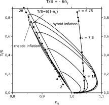
Figure 2 presents the corresponding T/S evaluated by means of the famous consistency relation T/S$\simeq-6n_{\rm T}$. The inflationary models, located along the line with solid circles (marked by ”c=…”), satisfy both observational tests mentioned above. Assuming that T/S is not large (T/S$<0.5$) we may constrain $n_{\rm S}$ ($1<n_{\rm S}<1.05$) and inflationary parameter $c$ ($c>8$).

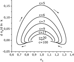
Recall that $n_{\rm S}$ is estimated at COBE scale and can change at different scales (for example, $n_{\sigma_{8}}$). Figure 3 demonstrates running parameter $\partial n_{\rm S}/\partial\ln k$. We see that the density perturbation slope at LSS scale ($k_{2}$) depends on $c$ and can vary from 1 till 1.2.

Figure 3: $\partial n_{\rm S}/\partial\ln k$ versus $n_{\rm S}$ in Lambda-inflation.

4 Discussion

The demonstrated example of $\Lambda$-inflation favors slightly blue spectra of density perturbations ($n_{\rm S}{}^{>}_{\sim}1$). However, phenomenological constraints for $n_{\rm S}$ based on LSS observational data, while converging to $n_{S}\simeq 1$, are still uncertain about the sign of ($n_{S}-1$). E.g., galaxy cluster data prefer $n_{S}>1$ $\!{}^{{\bf?}}$, whereas galactic surveys indicate slightly red spectra ($n_{\rm S}<1$) (e.g. $\!{}^{{\bf?}}$). Certainly, better data are required to delimit the slope of the fundamental spectrum. If future analysis reveals a blue spectrum, the $\Lambda$-inflation model will gain strong support as the theory of the very early Universe.

References

- [1] P. de Bernardis et al, Nature 404, 955 (2000).
- [2] A. Balbi et al, ApJ 545, L1 (2000).
- [3] C. Pryke et al, ApJ 568, 46 (2002).
- [4] see a talk given at this conference.
- [5] see a talk given at this conference.
- [6] V.N. Lukash, Sov.Phys.JETP 52, 807 (1980).
- [7] S. Hannestad et al, Astropart.Phys. 17, 375 (2002).
- [8] V.N. Lukash and E.V. Mikheeva, Int.J.Mod.Phys. A 15, 3783 (2000).
- [9] V.N.Lukash et al, MNRAS 317, 795 (2000).
- [10] A. Linde, Phys. Rev. D 49, 748 (1994).
- [11] B. Novosyadlyj et al, A&A 356, 418 (2000).