MHD Turbulence as a Foreground for CMB Studies

Abstract

Measurements of intensity and polarization of diffuse Galactic synchrotron emission as well as starlight polarization reveal power law spectra of fluctuations. We show that these fluctuations can arise from magnetohydrodynamic (MHD) turbulence in the Galactic disk and halo. To do so we take into account the converging geometry of lines of sight for the observations when the observer is within the turbulent volume. Assuming that the intensity of turbulence changes along the line of sight, we get a reasonable fit to the observed synchrotron data. As for the spectra of polarized starlight we get a good fit to the observations taking into account the fact that the observational sample is biased toward nearby stars.

1 Introduction

Attempts to determine the statistics of intensity and polarization fluctuations of cosmic microwave background (CMB) renewed interest to the fluctuations of Galactic foreground radiation (see Tegmark et al. 2000). Spectra of intensity of synchrotron emission and synchrotron polarization (see papers in de Oliveira-Costa & Tegmark 1999) as well as starlight polarization (Fosalba et al. 2002; henceforth FLPT) have been measured. Those measurements revealed a range of power-laws, the origin of which has not been addressed as far as we know. In Tegmark et al. (2000) there is an allusion that the spectra may be relevant to Kolmogorov turbulence, but the issue of how those different spectra may arise has not been addressed.

Interstellar medium is turbulent and Kolmogorov-type spectra were reported on the scales from several AU to several kpc (see Armstrong et al. 1995; Lazarian & Pogosyan 2000; Stanimirovic & Lazarian 2001). Therefore it is natural to think of the turbulence as the origin of the fluctuations of the diffuse foreground radiation. Interstellar medium is magnetized with magnetic field making turbulence anisotropic. It may be argued that although the spectrum of MHD turbulence exhibits scale-dependent anisotropy if studied in the system of reference defined by the local magnetic field (Goldreich & Sridhar 1995; Lithwick & Goldreich 2001; Cho & Lazarian 2002), in the observer’s system of reference the spectrum will show only moderate scale-independent anisotropy. Thus from the observer’s point of view Kolmogorov description of interstellar turbulence is acceptable in spite of the fact that magnetic field is dynamically important and even dominant (see discussion in Lazarian & Pogosyan 2000; Cho, Lazarian & Vishniac 2002).

It is customary for CMB studies to expand the foreground intensity over spherical harmonics $Y_{lm}$, $I(\theta,\phi)=\sum_{l,m}a_{lm}Y_{lm}(\theta,\phi)$, and write the spectrum in terms of $C_{l}\equiv\sum_{m=-l}^{m=l}|a_{lm}|^{2}/(2l+1)$. The measurements indicate that angular power spectra ($C_{l}$) of the Galactic emission follows power law ($C_{l}\propto l^{-\alpha}$) (see FLPT and references in §3).

This paper tests whether the measured spectra are compatible with the theoretical predictions of spatial statistics that is expected in the presence of MHD turbulence. Analytical studies in this direction were done in Lazarian (1992, 1994, 1995) and here we supplement them with numerical simulations of the synthetic spectra.

2 Spectra of Fluctuations

2.1 $C_{l}$ for small angle limit

In this section we show that, when the angle between the lines of sight is small (i.e. $\theta<L/d_{max}$), the angular spectrum $C_{l}$ has the same slope as the 3-dimensional energy spectrum of turbulence. Here $L$ is the typical size of the largest energy containing eddies, which is sometime called as outer scale of turbulence or energy injection scale, and $d_{max}$ is the distance to the farthest eddies (see Fig. 1a).

To illustrate the problem consider the observations with lines of sight being parallel. The observed intensity is the intensity summed along the line of sight, $r_{z}$.

$${I}_{2D}(r_{x},r_{y}) \equiv \int d{r_{z}}~{}i_{3D}({\bf r})$$ (1)

$$= \int d{r_{z}}\ \int dk_{x}dk_{y}dk_{z}\ \hat{i}_{3D}({\bf k})\ e^{i{\bf k}\cdot{\bf r}}.$$ (2)

Rearranging the order of summation and using $\int d{r_{z}}\ e^{ik_{z}r_{z}}=\delta(k_{z})$, we get

$${I}_{2D}(r_{x},r_{y})=\int d{k_{x}}dk_{y}~{}\hat{i}_{3D}(k_{x},k_{y},0)~{}e^{ik_{x}r_{x}+ik_{y}r_{y}},$$ (3)

which means Fourier component of ${I}_{2D}(r_{x},r_{y})$ is $\hat{i}_{3D}(k_{x},k_{y},0)$.

When the angular size of the observed region ($\Delta\theta\times\Delta\theta$ in radian) on the sky is small, $C_{l}$ is approximately the ‘energy’ spectrum of ${I}_{2D}(r_{x},r_{y})$ (Bond & Efstathiou 1987; Hobson & Majueijo 1996; Seljak 1997), which means $C_{l}\sim|\hat{i}_{3D}(k_{x},k_{y},0)|^{2}$ with $l\sim k(\pi/\Delta\theta)$ and $k=(k_{x}^{2}+k_{y}^{2})^{1/2}$. The analysis of the geometry of crossing lines of sight is more involved, but for power-law statistics it follows from Lazarian & Shutenkov (1990) that if $|\hat{i}_{3D}|^{2}\propto k^{-m}$, then the ‘energy’ spectrum of ${I}_{2D}(r_{x},r_{y})$ is also $k^{-m}$. Therefore, we have

$$C_{l}\propto|\hat{i}_{3D}(k_{x},k_{y},0)|^{2}\propto l^{-m}.$$ (4)

in the small $\theta$ limit.

For Kolmogorov turbulence ($|\hat{i}_{3D}|^{2}\propto k^{-11/3}$), we expect

$$C_{l}\propto l^{-11/3},\mbox{~{}~{}~{}if $\theta<L/d_{max}$.}$$ (5)

Note that $l\sim\pi/\theta$.

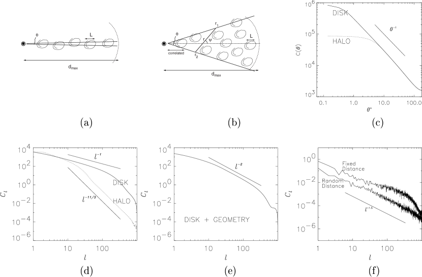
Figure 1: (a) Small $\theta$ limit ($\theta<L/d_{max}$). The fluctuations along the entire length of the lines of sight are correlated. (b) Large $\theta$ limit ($\theta>L/d_{max}$). Only points close to the observer are correlated. (c) Angular correlation function for disk (solid line) and for halo (dotted line). When $\theta$ is small, $K(\theta)\propto constant-\theta^{5/3}$. When $\theta$ is large, $K(\theta)\propto\theta^{-1}$. (d) Spectra for disk ($d_{max}$ = 10 kpc; turbulence size L = 100 pc) and for halo ($d_{max}$ = 1 kpc; turbulence size L = 100 pc). (e) Angular spectrum for Galactic disk. We considered geometry of Galactic disk. (f) Angular spectra of degree of polarization. Fixed Distance means all star are at the same distance. Random Distance means random sampling of stars according to equation (13). Zero point of the y-axis is arbitrary for all graphs.

2.2 $C_{l}$ for large angle limit

Following Lazarian & Shutenkov (1990), we can show that the correlation function for $\theta>L/d_{max}$,

$$K(\theta) = \int\int dr_{1}dr_{2}~{}{\cal K}(|{\bf r}_{1}-{\bf r}_{2}|),$$ (6)

$$= \frac{1}{\sin{\theta}}\int_{0}^{\infty}dr~{}r{\cal K}(r)\int_{0}^{\pi/2}d\psi\sim\frac{const}{\theta},$$

where we change variables: $(r_{1},r_{2})\rightarrow(r,\psi)$ is clear from Fig. 1b; we accounted for the Jacobian of which is $r/\sin{\theta}$. We can understand $1/\theta$ behavior qualitatively from Fig. 1b. When the angle is large, points along of the lines-of-sight near the observer are still correlated. These points extend from the observer over the distance $\propto 1/\sin{(\theta/2)}$.

In the limit of $\theta\ll 1$ we get the angular power spectrum $C_{l}$ using Fourier transform:

$$C_{l} \sim \int\int K(\theta)e^{-i{\bf l}\cdot{\bf\theta}}d\theta_{x}d\theta_{y}$$ (7)

$$\sim \int d\theta~{}\theta J_{0}(l\theta)K(\theta)\propto l^{-1},$$

where $\theta=(\theta_{x}^{2}+\theta_{y}^{2})^{1/2}$, $J_{0}$ is the Bessel function, and we use $K(\theta)\propto\theta^{-1}$.

In summary, for Kolmogorov turbulence, we expect from equations (5) and (7) that

$$C_{l}\propto\left\{\begin{array}[]{ll}l^{-11/3}&\mbox{if $l>l_{cr}$}\\ l^{-1}&\mbox{if $l<l_{cr}$.}\end{array}\right.$$ (8)

which means that the power index $\alpha$ of $C_{l}$ is $-1\leq\alpha\leq-11/3$. The critical number $l_{cr}~{}(\sim 3d_{max}/L)$ depends on the size of the size of the large turbulent eddies and on the direction of the observation. If in the naive model we assume that turbulence is homogeneous along the lines of sight and has $L\sim 100\ pc$ corresponding to a typical size of the supernova remnant for disk with $d_{max}\sim 10$ kpc, we get $l_{cr}\sim 300$. For the synchrotron halo, $d_{max}\sim 1$ kpc (see Smoot 1999) and we get $l_{cr}\sim 30$.

3 Synchrotron Radiation

Recent statistical studies of total synchrotron intensity include Haslam all-sky map at 408 MHz that shows that the power index $\alpha$ is in the range between 2.5 and 3 (Tegmark & Efstathiou 1996; Bouchet, Gispert, & Puget 1996). Parkes southern Galactic plane survey at 2.4 GHz suggests shallower slope: Giardino et al. (2002) obtained $\alpha\sim 2.05$ after point source removal and Baccigalupi et al. (2001) obtained $\alpha\sim-0.8$ to $-2$. Using Rhodes/HartRAO data at 2326 MHz, Giardino et al. (2001) obtained $\alpha\sim 2.43$ for all-sky data and $\alpha\sim 2.92$ for high Galactic latitude regions with $|b|>20^{o}$. The rough tendency that follow from these data is that $\alpha$ which is close to $2$ for the Galactic plane gets steeper (to $\sim-3$) for higher latitudes. In other words $-2\leq\alpha\leq-3$ which differs from naive expectations given by equation (8).

Can the difference be due to non-linear law of synchrotron emissivity? For synchrotron radiation, emissivity at a point ${\bf r}$, $i({\bf r})\propto n(e)|{B}_{\bot}|^{\gamma}$, where $n(e)$ is the electron number density, $B_{\bot}$ is the component of magnetic field perpendicular to the line of sight. The index $\gamma$ is approximately $2$ for radio synchrotron frequencies (see Smoot 1999). If electrons are uniformly distributed over the scales of magnetic field inhomogeneities, the spectrum of intensity reflects the statistics of magnetic field. For small amplitude perturbations ($\delta b/B\ll 1$; this is true for scales several times smaller than $L$ when we interpret $B$ as local mean magnetic field strength), if $\delta b$ has a power-law behavior, the statistics of intensity will have the same power-law behavior (see Deshpande et al. 2000). Therefore emissivity non-linearity does not account for the difference between the observed spectra and the theoretical expectations.

To address the problem, we perform simple numerical calculations for galactic disk and halo. We obtain $C_{l}$ using the relation

$$K(\cos\theta)=\frac{1}{4\pi}\sum_{l}(2l+1)C_{l}P_{l}(\cos{\theta}),$$ (9)

$$C_{l}=\frac{1}{2}\int P_{l}(\cos{\theta})K(\cos\theta)\ d(\cos\theta).$$ (10)

We use Gauss-Legendre quadrature integration (see Szapudi et al. 2001 for its application to CMB) to obtain $C_{l}$. We numerically calculate the angular correlation function from

$$K(\cos{\theta})=\int dr_{1}\int dr_{2}~{}{\cal K}(|{\bf r}_{1}-{\bf r}_{2}|),$$ (11)

where $|{\bf r}_{1}-{\bf r}_{2}|=r_{1}^{2}+r_{2}^{2}-2r_{1}r_{2}\cos{\theta}$ and assume that the spatial correlation function ${\cal K}(r)$ follow Kolmogorov statistics:

$${\cal K}(r)\propto\left\{\begin{array}[]{ll}{\cal K}_{0}-r^{2/3}&\mbox{if $r<L$}\\ 0&\mbox{if $r>L$,}\end{array}\right.$$ (12)

where ${\cal K}_{0}\sim L^{2/3}$ is a constant. Fig. 1c and Fig. 1d illustrate the agreement of our calculations with the theoretical expectations within the naive model of the disk and the halo from the previous section.

To make the spectrum closer to observations we need to consider more realistic models. First, synchrotron emission is stronger in spiral arms, and therefore we have more synchrotron emission coming from the nearby regions. Second, if synchrotron disk component is sufficiently thin, then lines of sight are not equivalent and effectively nearby disk component contributes more. Indeed, when we observe regions with low Galactic latitude, the effective line-of-sight varies with Galactic latitude.

Suppose we observe a region with $b=10^{o}$. Then emission from $d=10~{}kpc$ is substantially weaker than that from $d=100~{}pc$, because the region with $d=10~{}kpc$ is $10\ kpc~{}\sin{10^{o}}\sim 1.7~{}kpc$ above the Galactic plane and, therefore, has weak emission. To incorporate this effect, we use the weighting function $w(r)=100/max(100,r\sin{10^{o}})$, which gives more weight on closer distance. The resulting angular power spectrum (Fig. 1e) shows a slope similar to -2.

For halo, the simple model predicts that $C_{l}\propto l^{-11/3}$, but observations provide somewhat less steep spectra. Is this discrepancy very significant? The spectrum of magnetic field is expected to be shallower than $k^{-11/3}$ in the vicinity of the energy injection scale and at the vicinity of the magnetic equipartition scale. The observed spectrum also gets shallower if $d_{max}$ gets larger. For instance Beuermann, Kanbach, & Berkhuijsen (1985) reported the existence of thick radio halo that extends to more than $\sim 3~{}kpc$ near the Sun. Finally, filamentary structures and point sources can make the spectrum shallower as well. Further research should establish the true reason for the discrepancy.

4 Galactic Starlight Polarization

Polarized radiation from dust is an important component of Galactic foreground that strongly interferes with intended CMB polarization measurements (see Lazarian & Prunet 2001). FLPT attempted to predict the spectrum of the polarized foreground from dust and obtained $C_{l}\sim l^{-1.5}$ for starlight polarization. This spectrum is different from those discussed in the previous sections. To relate this spectrum to the underlying turbulence we should account for the following facts: a) the observations are done for the disk component of the Galaxy, b) the sampled stars are at different distances from the observer with most of the stars close-by.

To deal with this problem we use numerical simulations again. We first generate a three (i.e. x,y, and z) components of magnetic field on a two-dimensional plane ($4096\times 4096$ grid points representing $10~{}kpc\times 10~{}kpc$), using the following Kolmogorov three-dimensional spectrum: $E_{3D}(k)\propto k^{-11/3}$ if $k>k_{0}$, where $k_{0}\sim 1/100~{}pc$. Our results show that how we continuously extend the spectrum for $k<k_{0}$ does not change our results.

To simulate the actual distribution of stars within the sample used in FLPT, we scatter our emission sources using the following probability distribution function:

$$P(r)\propto e^{-r/1.5kpc}.$$ (13)

The starlight polarization is due to the difference in absorption cross section of non-spherical grains aligned with their longer axes perpendicular to magnetic field (see review by Lazarian 2000). In numerical calculations we approximate the actual turbulent magnetic field by a superposition of the slabs with locally uniform magnetic field in each slap and assume that the difference in grain absorption parallel and perpendicular to magnetic field results in the 10% difference in the optical depths $\tau_{\|}$ and $\tau_{\bot}$ for a slab. We calculate evolution of Stocks parameters of the starlight within the slab and use the standard transforms of Stocks parameters from one slab to another (Dolginov, Gnedin, & Silantev 1996; see similar expressions in Martin 1972).

We show the result in Fig. 1f. For comparison, we also calculate the degree of polarization assuming all stars are at the same distance of $\sim 10~{}kpc$. The result shows that, for a mixture of nearby and faraway stars, the slope steepens and gets very close to the observed one, i.e. $-1.5$.

Our conclusions may be tested if stars at particular distance only are correlated. If those stars are nearby, we would expect to have steeper index and it will become shallow if only distant stars are chosen. Choosing only nearby stars we expect to get a steeper index. A systematic study of this change can provide an estimate of the energy injection scale $L$. From the point of view of foreground studies, we conclude that a naive use of the polarization template produced with the random sample of stars may be misleading.

5 Summary

In this paper we have addressed the origin of spatial fluctuations of emissivity and polarization of Galactic diffuse emission. We have shown that MHD turbulence can qualitatively explain observed properties of total synchrotron emission and starlight polarization. The variety of measured spatial spectra of synchrotron emission can be explained by the inhomogeneous distribution of emissivity, structure of Galactic disk and halo, and/or various energy injection scales. Similarly, MHD turbulence plus inhomogeneous distribution of stars can explain the reported scaling of starlight polarization statistics.

Evidently more systematic studies are required. Those studies will not only give insight into how to separate CMB from foregrounds, but also would provide valuable information on the structure of interstellar medium and the sources/energy injection scales of interstellar turbulence.

References

- (1) Armstrong, J. W., Rickett, B. J., & Spangler, S. R. 1995, ApJ, 443, 209
- (2)
- (3) Bond, J.R. & Efstathiou, G. 1987, MNRAS, 226, 655
- (4)
- (5) Bouchet, F.R., Gispert, R., & Puget, J.L. 1996, in Unveiling the Cosmic Infrared Background, AIP Conf. Proc. 348, ed. E. Dwek (Baltimore: AIP), 225
- (6) Beuermann, K., Kanbach, G., & Berkhuijsen, E. 1985, A&A, 153, 17
- (7)
- (8) Cho, J. & Lazarian, A. 2002, Phy. Rev. Lett., submitted
- (9) Cho, J., Lazarian, A., & Vishniac, E. T. 2002, in Simulations of magnetohydrodynamic turbulence in astrophysics, eds. by T. Passot & E. Falgarone (Springer Lecture Notes in Physics; 2002), submitted
- (10)
- (11) de Oliveira-Costa, A. & Tegmark, M. 1999, Microwave Foregrounds, ASP Conf. Ser. 181, (San Francisco: ASP)
- (12)
- (13) Deshpande, A.A., Dwarakanath, K.S., Goss, W.M., 2000, ApJ, 543, 227
- (14)
- (15) Dolginov, A. Z., Gnedin, Iu. N., & Silantev, N. A. 1996, Propagation and polarization of radiation in cosmic media, (Gordon & Breech)
- (16) Fosalba, P., Lazarian, A., Prunet, S., & Tauber, J.A. 2002 ApJ, 564, 762 (FLPT)
- (17)
- (18) Giardino, G., Banday, A.J., Fosalba, P., Górski, K.M., Jonas, J.L., O’Mullane, W., & Tauber, J. 2001, A&A, 371, 708
- (19)
- (20) Giardino, G., Banday, A.J., Górski, K.M., Bennett, K., Jonas, J.L., & Tauber, J. 2002, A&A, astro-ph/0202520
- (21)
- (22) Goldreich, P. & Sridhar, H. 1995, ApJ, 438, 763
- (23)
- (24) Hobson, M.P. & Magueijo, J. 1996, MNRAS, 283, 1133
- (25)
- (26) Lazarian, A. 1992, Astron. & Astrophys. Trans., 3, 33
- (27) Lazarian, A. 1994, Ph. D. Thesis (Univ. of Cambridge, UK)
- (28) Lazarian, A. 1995, A&A, 293, 507
- (29) Lazarian, A. 2000, in Cosmic Evolution and Galaxy Formation, ASP v.215, ed. by J. Franco, E. Terlevich, O. Lopez-Cruz, I. Aretxaga (Astron. Soc. Pacific) p.69 (astro-ph/0003414)
- (30) Lazarian, A. & Pogosyan, D. 2000, ApJ, 537, 720L
- (31) Lazarian, A. & Prunet, 2001, in Microwave Foregrounds, ASP Conf. Ser. 181, (San Francisco: ASP), p32
- (32) Lazarian, A. & Shutenkov, V. P. 1990, Sov. Astron. Lett., 16, 297
- (33)
- (34) Lithwick, Y. & Goldreich, P. 2001, ApJ, 562, 279
- (35)
- (36) Martin, P. G. 1972, MNRAS, 159, 179
- (37)
- (38) Seljak, U. 1997, ApJ, 482, 6
- (39) Smoot, G. F. 1999, in Microwave Foregrounds, ASP Conf. Ser. 181, ed. A. de Oliveira-Costa & M. Tegmark (San Francisco: ASP), 61
- (40)
- (41) Stanimirovic, S., & Lazarian, A. 2001, ApJ, 551, L53
- (42) Szapudi, I., Prunet, S., Pogosyan, D., Szalay, A. S., & Bond, J. R. 2001, ApJ, 548, L115
- (43)
- (44) Tegmark, M. & Efstathiou, G. 1996, MNRAS, 281, 1297
- (45) Tegmark, M., Eisenstein, D. J., Hu, W., de Oliveira-Costa, A. 2000, ApJ, 530, 133