General Relativistic Geodetic Spin Precession in Binary Pulsar B1913+16: Mapping the Emission Beam in Two Dimensions

Abstract

We have carefully measured the pulse profile of the binary pulsar PSR B1913+16 at 21 cm wavelength for twenty years, in order to search for variations that result from general relativistic geodetic precession of the spin axis. The profile width is found to decrease with time in its inner regions, while staying essentially constant on its outer skirts. We fit these data to a model of the beam shape and precession geometry. Four equivalent solutions are found, but evolutionary considerations and polarization data select a single preferred model. While the current data sample only a limited range of latitudes owing to the long precessional cycle, the preferred model shows a beam elongated in the latitude direction and hourglass–shaped.

1 Introduction

The binary pulsar PSR B1913+16 resides in the strong gravitational field of its companion. As a result, a wide variety of relativistic phenomena are observable, including advance of periastron, gravitational redshift, and, most notably, orbital decay due to gravitational radiation emission (Taylor & Weisberg 1989; Taylor et al. 1992). Here we report on an additional general relativistic phenomenon, the gravitomagnetic spin–orbital coupling known as geodetic precession. This precession provides a unique opportunity to study the pulsar beam along the latitude direction, orthogonal to the usual longitude dimension revealed by pulsars’ spinning across our line of sight.

Geodetic precession and resulting pulseshape changes in PSR B1913+16 were predicted shortly after the pulsar’s discovery in 1974 (Damour & Ruffini 1974; Barker & O’Connell 1975a,b; Esposito & Harrison 1975). The expected signature of this phenomenon would be a change in the longitude separation of the two main pulse components, which are thought to be emitted from opposite sides of a hollow cone, as the line of sight slowly precesses across the cone. The first observational searches for evidence of geodetic precession were reported by Weisberg, Romani, & Taylor (1989) and Weisberg & Taylor (1992). The expected component separation variation was not observed, although a secular change in the relative intensity of the two main components was detected. These observations were interpreted by the authors as resulting from our line of sight fortuitously precessing across the middle (to explain the constancy of component separation) of a patchy (to justify the relative intensity variation) emission beam. Istomin (1991) then predicted on the basis of these observations that the beam will precess out of our line of sight in the year $\sim 2020$. The expected component separation change was finally detected by Kramer (1998), using data from the Effelsberg 100–m dish combined with our earlier results. Kramer used data on the separation between the two profile peaks as a function of time to fit a model for the geometry of the precession and of the beam. Here we augment our earlier measurements with new Arecibo post–upgrading observations over the last few years. We measure the beamwidth as a function of time at fourteen different intensity levels, and we fit these data to a model of the beam geometry to arrive at a picture of the two–dimensional structure of the emission region.

2 Data Acquisition

All data were gathered at Arecibo Observatory at frequencies near 1400 MHz with one of a series of dedicated pulsar backends, called the Mark I, II, and III systems [see Taylor & Weisberg (1989) for details]. In all cases, two orthogonal circularly polarized signals were sampled, detected, dedispersed, folded at the apparent pulsar period, and integrated on–line for five minutes. The resulting total power pulse profile was stored to tape as the basic processing unit, a “scan.”

The scans from a given observing session, typically consisting of fourteen 2–3 h daily blocks of data acquisition, were then summed to create a “session–average” profile. All subsequent analyses used these twenty–two session average profiles, acquired between 1981 and 2001.

In order to make the Mark I, II, and III data as closely intercomparable as possible, we simulated in software some of the on-line hardware. We chose to smooth the Mark I and II data to match the coarser resolution of the Mark III system, with its $312\,\mu s$ exponential time constant, 1.25 MHz individual frequency channels, and 512 phase bins. (The Mark I and Mark II data had already been made effectively equivalent by convolving the Mark II data with a $100\,\mu s$ time constant(Weisberg et al., 1989). The Mark I and equivalent Mark II data were convolved with a decaying exponential function of $300\,\mu s$ time constant to match the Mark III hardware exponential time constant, and with an 11-bin ($650\,\mu s$) boxcar function to simulate the dispersion smearing across the individual Mark III filter channels. Adjacent pairs of the resulting 1024–bin waveform were combined to create final 512–bin Mark I and Mark II profiles equivalent to the Mark III profiles.

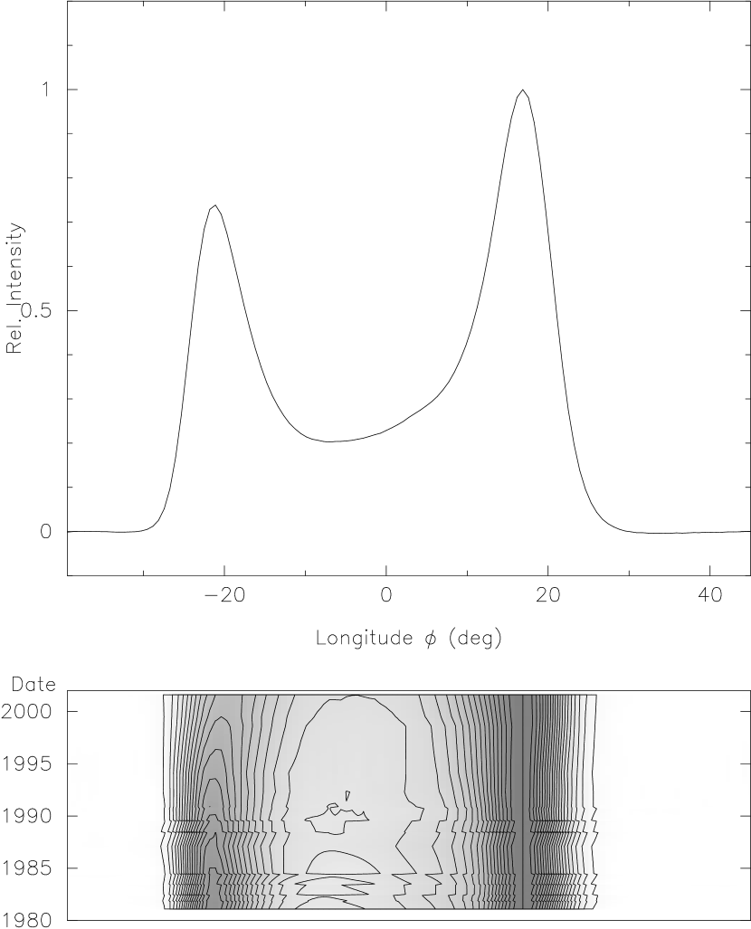
Figure 1: PSR B1913+16 Pulse Profile. Top: time–averaged profile. Bottom: Equal–intensity contour plot, as a function of longitude and time. The right peak normalized to constant (unity) intensity, and set at fixed longitude. Note that the left peak of the profile declines in intensity and approaches the right peak while the central saddle fills in and the outer skirts of the profile barely change through the timespan of observations.

Fig. 1 shows the resulting profiles as a function of time, displayed as a contour plot with the right peak arbitrarily normalized to constant longitude and intensity. There are several notable items revealed in the Fig. 1 contour plot. First, the leading– to trailing–component peak intensity ratio $(I_{leading}/I_{trailing})$ continued its secular decline of $\sim 1\%/$ yr, which Weisberg et al. (1989) attributed to our line of sight slowly precessing across a patchy beam. In addition, the peaks have clearly been moving together with time in the last decade, as first announced by Kramer (1998). Furthermore, it is evident that the saddle is filling in with time. Surprisingly, however, the separation and shape of much of the profile outside the peaks remain virtually unchanged over the twenty-year timespan of data. While precession across a circular, hollow–cone beam would naturally be expected to result in more pronounced changes on its inner portions where the radius of curvature is small than on its outer segments, we will show below that our data cannot be explained in this fashion alone. Instead we will find from model fits that the beam must be elongated in the meridional (i.e., north–south) direction, and hourglass–shaped.

3 Analysis

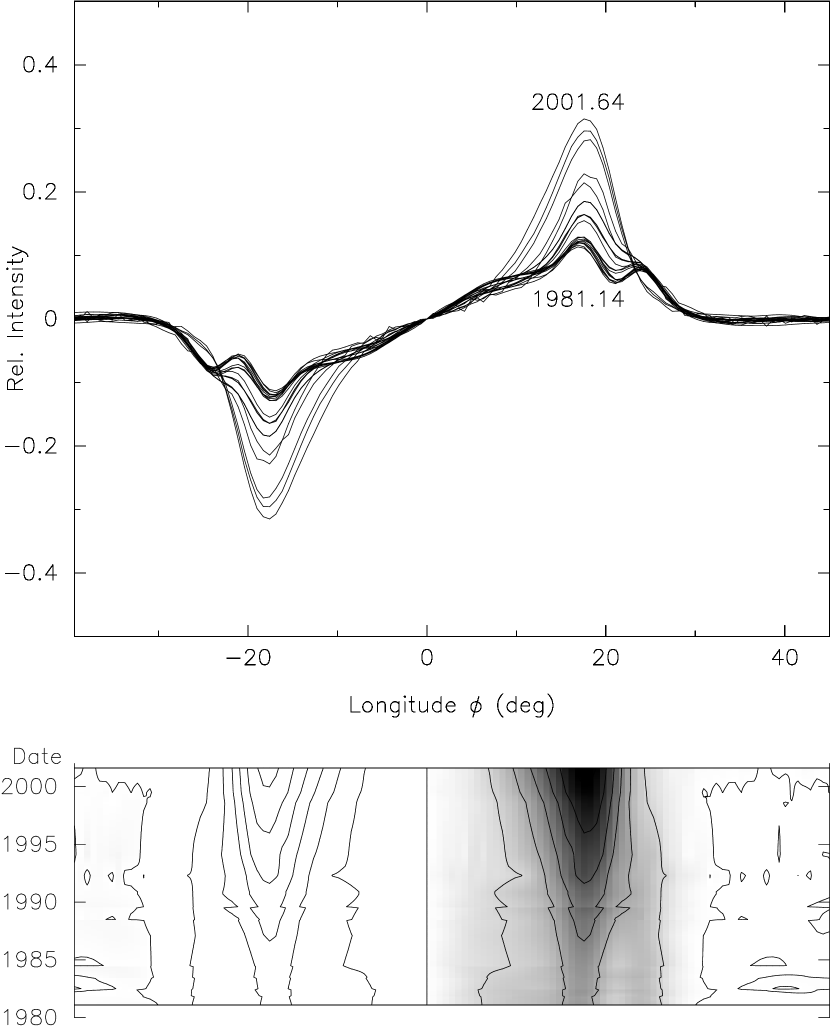
Figure 2: Odd Component of PSR B1913+16 Pulse Profile. Top: Individual session profiles. Bottom: Equal–intensity contour plot, as a function of longitude and time.

Following up on our finding that our line of sight is slowly precessing across a patchy beam, we decomposed each epoch’s profile into an odd and an even part, associating the former with the beam patchiness and the latter with the overall hollow–cone beam structure. Figs. 2 and 3 display the odd and even components, respectively. All subsequent global beam analysis was performed on the even parts alone. The pulsar beamwidth $w$ at various intensity levels was determined from these even profiles, providing the raw data for the analysis (see below).

3.1 The Beam Model

In our model, the beam half–width $\rho_{j}$ for a given $j-th$ constant intensity level is a function of scale factor $s$ (of order unity); fiducial half–width $\rho_{0,j}$; elongation parameters $R$ and $a$; and north–south (i.e., meridional) offset from beam axis $t$; as follows:

$$\rho_{j}=s\rho_{0,j}(1+\frac{(R-1)t^{2}}{a^{2}+t^{2}}).$$ (1)

Of the two elongation parameters, $R$ is essentially the axial ratio of the elongated beam, i.e., approximately the ratio of its north–south to east–west extent; while $a$ gives a $t$–dependent adjustment on the shape.

3.2 The Geometrical Model

Eq. 1 alone is not sufficient to relate our measured $w$’s in longitude units to our beam model, because we do not know the full observing geometry a priori. For example, the angle of the beam axis with respect to the observer, to the spin axis, and to the orbital axis are unknown. [Note that the sine of the orbital inclination, $\sin i$, is already known from pulse timing measurements (Taylor & Weisberg, 1989), as discussed below.]

Consequently we have to fit simultaneously for several additional geometrical quantities in addition to the elongated beam quantities delineated in Eq. 1. In what follows we will use the work of Kramer (1998) as a general guide, but we will adhere to a right–handed coordinate system notation as in Damour & Taylor (1992) and Everett & Weisberg (2001). (See Fig. 4.) The inclination $i$ is the angle between the orbital angular momentum vector $\vec{J}_{orb}$; and the line of sight vector from the observer to the pulsar, $\hat{K}$. The spin–orbit misalignment angle $\lambda$ is measured between $\vec{J}_{orb}$ and the pulsar spin angular momentum vector $\hat{\Omega}_{psr}(t)$, also called the north spin pole. Geodetic precession of $\hat{\Omega}_{psr}(t)$ about $\vec{J}_{orb}$ occurs in the $\vec{J}_{orb}\times\hat{\Omega}_{psr}(t)$ direction at a rate of $\Omega_{prec}=1.213\deg/$ yr [See Barker & O’Connell (1975a,b); Weisberg et al. (1989) for the formula]. The emission beam colatitude $\alpha$ is the angle between $\hat{\Omega}_{psr}(t)$ and the visible magnetic axis $\hat{\mu}$, while line–of–sight colatitude $\zeta(t)$ is the angle between $\hat{\Omega}_{psr}(t)$ and the line of sight from the pulsar to observer $\hat{n}$, where $\hat{n}=-\hat{K}$.

Now set up a right–handed coordinate system $(\hat{x},\hat{y},\hat{z})$ where $\hat{z}$ points along the orbital angular momentum $\vec{J}_{orb}$; and the $\hat{x}$–vector points such that the plane defined by the $\hat{x}$– and $\hat{z}$– vectors contains the observer–pulsar line–of–sight vector $\hat{K}$ (with $\hat{x}$ pointing more toward $\hat{K}$ than toward its opposite, $\hat{n}$). The reference time $T_{0}$ is defined as the time when the (precessing) spin angular momentum vector $\hat{\Omega}_{psr}(t)$ lies in this same plane containing $\hat{x}$ and $\hat{z}$ (and $\hat{K}$) and points most directly toward $\hat{x}$ and away from the observer. We can then define a precessional phase $\phi_{prec}(t)=\Omega_{prec}(t-T_{0})$. The position of the precessing spin axis, $\hat{\Omega}_{psr}(t)$, can be resolved onto the Cartesian coordinate system as follows:

$$\hat{\Omega}_{psr}(t)=\hat{x}\cos\phi_{prec}(t)\sin\lambda+\hat{y}\sin\phi_{prec}(t)\sin\lambda+\hat{z}\cos\lambda;$$ (2)

while $\hat{K}$ is resolved onto the same system as

$$\hat{K}=\hat{x}\sin i+\hat{z}\cos i.$$ (3)

The observer’s line of sight colatitude $\zeta(t)$ can then be found at any epoch because the definition of the dot product requires that

$$\cos\zeta(t)=\hat{\Omega}_{psr}(t)\cdot\hat{n}=\hat{\Omega}_{psr}(t)\cdot(-\hat{K}),$$ (4)

so that we have

$$\cos\zeta(t)=-\cos\phi_{prec}(t)\sin\lambda\sin i-\cos\lambda\cos i.$$ (5)

Finally, $\beta(t)$, the impact parameter of the pulsar–observer line of sight $\hat{n}$ with respect to the visible magnetic axis $\hat{\mu}$, is given by

$$\beta(t)=\zeta(t)-\alpha.$$ (6)

3.3 Beam / Geometrical Model Fits

For our quantitative beam modelling, we first determined the pulse width $w$ at fourteen intensity levels $I_{j}$ for each of twenty-two epochs in the even profiles, and we then fitted to these data the elongated, north–south symmetric beam model of Eq. 1 plus the geometrical model delineated in the last section. The fourteen $\rho_{0,j}$ were fixed at values determined iteratively to optimize the fits described below. The orbital inclination $i$ was fixed at a value of $47\fdg 20$ or its supplement, as determined from pulse timing measurements of $\sin i$. The quantities $\alpha,\lambda,T_{0},s,R,$ and $a,$ were then determined from a weighted least–squares fitting procedure. Kramer (1998) also fitted for quantities similar to the first three and four of these parameters with his azimuthally symmetric beam model and data on the separation between the profile peaks only. We are able to fit for two additional parameters quantifying the shape of the beam because of our measurements of beamwidth at many different intensity levels, rather than only at the profile peaks.

As also found by Kramer (1998), there are four equivalent beam solutions: Two of them result from the ambiguity in $i$ discussed above, based on the fact that pulse timing yields $\sin i$. Then each of these two solutions is also degenerate in that $(\alpha,\lambda,T_{0})$ and $(\pi-\alpha,\pi-\lambda,T_{0}-\pi/\Omega_{prec})$ are indistinguishable. Fig. 5 displays the measured pulse widths, and the contours of constant intensity resulting from our final best fits to these data. (All four of the degenerate fits yield the same results on this figure, which is why they are degenerate.)

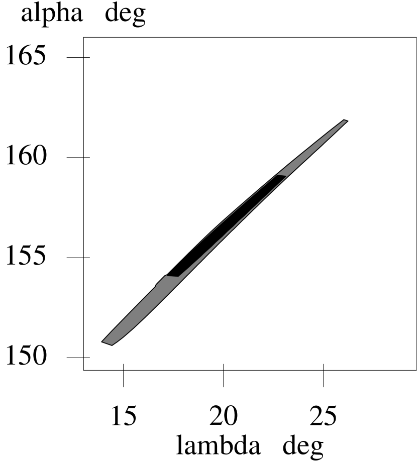
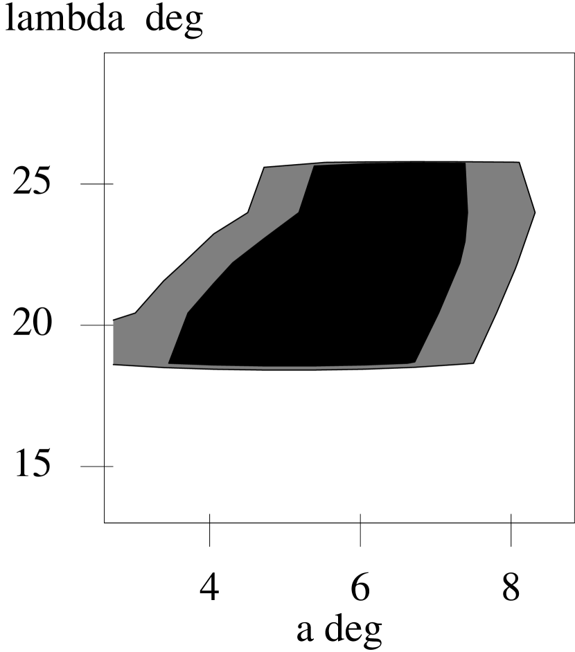
Figure 6: Contours of equal $\Delta{\chi}^{2}$, holding two parameters fixed at the values indicated on each graph and allowing all other parameters to be fitted. In both graphs, the inner contour is at the $\Delta{\chi}^{2}=1$ level; the outer is at $\Delta{\chi}^{2}=2$ above the best fit value.

Fortunately we can rule out the two high–$\lambda$ solutions because of evolutionary considerations: The spin and orbital angular momentum vectors were almost certainly aligned due to mass exchange before the last supernova occurred, and asymmetries in that explosion that would misalign the two vectors are constrained by the observed pulsar velocity distribution (Bailes 1988; Kramer 1998; Wex et al 2000). Table 1 records quantitatively the two surviving low–$\lambda$ fits. Because some of the fitted parameters are highly covariant, the formal errors must be read with caution. In order to further examine the uncertainties in fitted quantities, we explored $\chi^{2}$–space two parameters at a time in the following fashion. We stepped the two chosen parameters through a grid of values in the vicinity of the $\chi^{2}$–minimum, holding them fixed at each grid point while allowing all other parameters to be fitted. The resulting $\chi^{2}$ at each such grid point was then calculated and a contour map of $\chi^{2}$ as a function of the two parameters was generated. We display the two maps showing the most serious covariance in Fig. 6. Note especially that $\chi^{2}$ contours associated with $\alpha$ and $\lambda$ indicate that the possible range of their errors is much larger than indicated in our formal uncertainties.

3.4 Polarization Data and the Rotating Vector Model

In an effort to provide additional information on the emission beam geometry, we have also measured the polarization properties of the pulse profile starting with our 1998 observing session, using the Princeton Mark IV backend (Stairs et al., 2000). Early pulsar observations revealed a characteristic $S$–shaped sweep of polarization position angle across many pulse profiles. According to the rotating vector model (RVM) of Radhakrishnan & Cooke (1969), this signature can be understood as the projection of the rotating neutron star’s magnetic field lines onto the observer’s line of sight, because the emission is locally polarized in (or perpendicular to) the plane of the field lines. In theory, it is possible to fit linear polarization position angle data to the RVM in order to derive the emission beam geometry. In practice, however, it has been shown that unambiguous geometrical solutions from RVM fits to linear polarization data are rare, for two principal reasons (Everett & Weisberg, 2001): First, the observable emission from most pulsars occupies such a narrow longitude range that RVM fit parameters are highly covariant; and second, many pulsars’ emission does not conform simply to the RVM itself. Our polarized profiles (Fig. 7), indeed exhibit a complicated form. Cordes, Wasserman, & Blaskiewicz (1990) also measured and remarked on the complicated nature of the position angle curve. They noted that its overall sweep of $\sim 195\arcdeg$ is not allowed in the rotating vector model, and that the rapid swings indicate switching between orthogonal emission modes. These features have prevented us from being able to perform RVM fits to the position angle data that yield unique values for geometric parameters.

Despite these complications, the position angle data do provide critical information that enables us to select one and reject one of our two remaining beam model solutions. To do so, we calculated position angle curves for the best–fitting parameter values of both solutions listed in Table 1. For each solution, we first calculated the observers’ line of sight colatitude for the observing epoch $\zeta(t)$, from Eq. 5. We then determined the expected RVM linearly polarized position angle $\psi$ with longitude $\phi$ curve from the classic RVM equation [corrected for signs; see Everett & Weisberg (2001)]:

$$\tan(\psi-\psi_{0})=-\frac{\sin\alpha\sin(\phi-\phi_{0})}{\sin\zeta\cos\alpha-\cos\zeta\sin\alpha\cos(\phi-\phi_{0})}.$$ (7)

Note that $\alpha$ and $\zeta(t)$ go to their supplements in the alternate solutions, which also causes the impact parameter $\beta(t)$ to flip sign (see Eq. 6). This has crucial implications for the RVM and the polarized profile, since the slope of the polarized linear position angle curve, $d\psi/d\phi=-\sin\alpha/\sin\beta$ at the center of the pulse, also changes sign because our line of sight moves from one side of the magnetic axis to the other [see Everett & Weisberg (2001) for details].

The results for both solutions are shown in Fig. 7 atop the data. As expected, one model (Solution 2, with $\alpha\sim 22\arcdeg;\zeta\sim 29\arcdeg;\beta\sim 6\arcdeg$) clearly gives a grossly wrong position angle sweep with the wrong sign. The complementary model, (Solution 1, $\alpha\sim 158\arcdeg;\zeta\sim 151\arcdeg;\beta\sim-6\arcdeg$) sweeps in position angle in the same sense as the data.

It appears especially heartening that Solution 1 matches the observed position angles in the central regions of the pulse, not just in the sign of the slope but also in a more detailed fashion. As a result, we closely studied the position angle measurements in our data as well as the earlier polarimetry of Cordes et al (1990). The precession should cause the position angle curve to vary with time as $\zeta$ changes. The predicted changes are rather small over the timespan of our Mark IV data. However, we were disappointed to note that the Cordes et al. data from epoch 1988.5, which should show a position angle curve measurably different from current data, do not. Rather, the much earlier Cordes et al. position angle curve is essentially indistinguishable from our Mark IV curves to within the noise. We conclude that the pulsar’s emission is not following the RVM in detail. Nevertheless, it seems likely that the slope of the position angle curve near the symmetry axis of the pulse should still be related to the apparent rotation of the magnetic field lines emanating from the magnetic pole as they sweep across our line of sight, and hence successfully chooses the sign of $\beta$ and thus Solution 1.

4 Discussion

The fitted equal–intensity contours alone, without the data, are shown in Fig. 8, over a much larger north–south range than we have directly observed. We delineate the portion of the beam that we have directly sampled over the past twenty years with two horizontal lines. Note that we have observed only a small part of the beam in the vertical direction. Consequently our model is by no means unique, and it is probably incorrect in its details. Most notably, our assumption of north–south beam symmetry is currently untestable since all observations probe only the northern side of the beam. Nevertheless it is clear that any successful beam model must be able to match the striking features shown in the data and in our model: a shrinkage with time of the inner and peak equal–intensity contours, combined with uniform or even slightly growing outer contour widths.

The apparent north-south asymmetry in Fig. 8 is an artefact of displaying the horizontal axis in directly measurable longitude units (where $360\arcdeg=1$ pulsar rotation), which are portions of small circles whose arc length varies as one approaches a pole. Fig. 9 displays the best fitting beam model in true great–circle arc units on both axes, and the expected north–south (and east–west) symmetries are evident in this display. It is surprising that the beam takes on an ”hourglass” shape in order to match our observations of pulsewidth that varies strongly at small radii and remains virtually unchanged or even growing slightly at larger radii. It is interesting to note that Link & Epstein (2001) have also derived an hourglass–shaped beam for PSR B1828-11, an isolated pulsar that is also undergoing spin axis precession. Thus the only two pulsars whose beams have been mapped in the meridional direction show qualitatively similar beamshapes.

Others have investigated pulsar beamshapes. Most studies are based on rather indirect observational arguments, usually involving analyses of position angle and pulsewidth data in the pulsar population. Jones (1980) and Narayan & Vivekanand (1983) found significant north–south beam elongation. However, Lyne & Manchester (1988) and Bjoernsson (1998) indicated that the emission is consistent with a circular cone. Mitra & Deshpande (1999) also supported circular cones although finding marginal evidence for meridional compression. Biggs (1990) and McKinnon (1993) also point out that the beam will be meridionally compressed if its boundary is defined by the last closed field lines in a spinning neutron star with a tilted magnetic axis.

There is clearly no consensus on the overall beam elongation. In addition, we are not aware of any observational or theoretical studies indicating the hourglass shape, other than ours and Link & Epstein (2001).

5 Conclusion

We have used twenty years of pulse profile measurements on PSR B1913+16 to detect geodetic precession of the spin axis and to model the emission beam geometry. Evolutionary considerations and polarization measurements enable us to choose a single preferred model from four equivalent solutions. While we have only sampled a limited portion of the beam to date, our model indicates that the beam is elongated and hourglass–shaped in the latitude direction. Future observations will enable us to study the two dimensional beam structure at larger impact parameters, further constraining the details of the beamshape.

Figure 3: Even Component of PSR B1913+16 Pulse Profile. Top: time–averaged profile. Bottom: Equal–intensity contour plot, as a function of longitude and time. As in Fig. 1, note that the profile peak separation decreases while the central saddle fills in and the outer skirts remain virtually unchanged or even spread slightly through the observing timespan.

Figure 4: Precession geometry. The dashed ellipse shows the trajectory of the pulsar spin angular momentum vector $\hat{\Omega}_{psr}(t)$ resulting from geodetic precession. The vector is shown for epoch $T_{0}$. The pulsar–spin–induced trajectory of the observable magnetic pole $\hat{\mu}$ about $-\hat{\Omega}_{psr}(t)$ is shown, also for epoch $T_{0}$, as a dotted ellipse. All angles correspond qualitatively to those we find through model fitting (see text).

Figure 5: Even component pulsewidth versus time at the fourteen relative intensity levels listed on the contours. The points and error bars represent our data (also shown as contours at the bottom of Fig. 3); the curves display the model fitted to these data.

Figure 7: Polarization profiles at 1403 MHz in 1998 (left), and 1999 (right). In each plot, the top panel shows the polarized profile, with total power Stokes parameter $I$ the highest profile curve; linear power $L$ the next highest; and circularly polarized Stokes parameter $V$ dotted. The bottom panel displays the position angle as observed and as expected from applying the two low–$\lambda$ beam – geometrical fits listed in Table 1 to the rotating vector $(RVM)$ model of polarization. Solution 1 yields the smooth solid curve, while solution 2 leads to the smooth dashed curve. Each model was derived from beamshape data independent of polarization. For each epoch, one model conforms at least crudely to the position angle data while one is grossly wrong even in the sign of its slope. Note: The position angle $\psi$ conforms to the observers’ convention, increasing counterclockwise on the sky. The RVM model is cast in terms of a position angle $\psi^{\prime}(=-\psi)$ that increases clockwise on the sky (Everett & Weisberg, 2001).

Figure 8: The best–fitting, even component beam model, plotted as a function of longitude and north–south angular offset from the beam center. (Longitude is a direct measurable, since $360\arcdeg=1$ pulsar rotation.) The peak $(1.0)$ intensity contour is bold, and decreasing contours inside it are dashed. The apparent north–south beam asymmetry is due to the convergence of meridians (lines of constant longitude) toward the pole. See Fig. 9 for a view of the model in undistorted (great–circle arc) space. Currently we have directly sampled only those portions of the beam lying between the two horizontal lines. Note that this region of the plot is also displayed in the bottom of Fig. 3 and in Fig. 5. (The earlier figures show pulsewidth as a function of time, whereas we have used our fitted geometrical parameters to transform the time axis into an angular north–south offset on the pulsar in the above figure.)

Figure 9: The best–fitting, even component beam model, plotted as a function of east–west and north–south angular offset from the beam center. The peak $(1.0)$ intensity contour is bold, and decreasing contours inside it are dashed.

.

Table 1: Preferred Low–$\lambda$ Beam and Geometrical Model Solutions.

Para-	Description	Solution 1	Solution 2
meter
$i$	Orbital inclination	$47\fdg 2$	$132\fdg 8$(fixed)
$\alpha$	Emission beam colatitude	$157\fdg 5$	$22\fdg 5\pm 0\fdg 3$
$\lambda$	Spin–orbit misalignment angle	$21\fdg 1$	$21\fdg 1\pm 0\fdg 3$
$T_{0}$	Reference epoch	1981.0	$2129.4\pm 0.3$
$s$	Scale factor	1.04	$1.04\pm 0.01$
$R$	Axial ratio	1.59	$1.59\pm 0.02$
$a$	Shape adjustment	$5\fdg 57$	$5\fdg 57\pm 0\fdg 11$

Note. — Fits of the rotating vector model (RVM) to our polarization data eliminate Solution 2. See text and Fig. 7.

References

- Bailes (1988) Bailes, M. 1988, A&A, 202, 109
- Cordes, Wasserman, & Blaskiewicz (1990) Cordes, J. M., Wasserman, I., & Blaskiewicz, M. 1990, ApJ, 349, 546
- Barker & O’Connell (1975a,b) Barker, B. M. & O’Connell, R. F. 1975a, Phys. Rev. D, 12, 329
- Barker & Oconnell (1975b) Barker, B. M. & Oconnell, R. F. 1975b, ApJ, 199, L25
- Biggs (1990) Biggs, J. D. 1990, MNRAS, 245, 514
- Bjoernsson (1998) Bjoernsson, C.-I. 1998, A&A, 338, 971
- Damour & Ruffini (1974) Damour, T. & Ruffini, R. 1974, Academie des Sciences Paris Comptes Rendus Serie Sciences Mathematiques, 279, 971
- Damour & Taylor (1992) Damour, T. & Taylor, J. H. 1992, Phys. Rev. D, 45, 1840
- Esposito & Harrison (1975) Esposito, L. W. & Harrison, E. R. 1975, ApJ, 196, L1
- Everett & Weisberg (2001) Everett, J. E. & Weisberg, J. M. 2001, ApJ, 553, 341
- Istomin (1991) Istomin, Y. N. 1991, Soviet Astronomy Letters, 17, 301
- Jones (1980) Jones, P. B. 1980, ApJ, 236, 661
- Kramer (1998) Kramer, M. 1998, ApJ, 509, 856
- Lai, Chernoff, & Cordes (2001) Lai, D., Chernoff, D. F., & Cordes, J. M. 2001, ApJ, 549, 1111
- Link & Epstein (2001) Link, B. & Epstein, R. I. 2001, ApJ, 556, 392
- Lyne & Manchester (1988) Lyne, A. G. & Manchester, R. N. 1988, MNRAS, 234, 477
- McKinnon (1993) McKinnon, M. M. 1993, ApJ, 413, 317
- Mitra & Deshpande (1999) Mitra, D. & Deshpande, A. A. 1999, A&A, 346, 906
- Narayan & Vivekanand (1983) Narayan, R. & Vivekanand, M. 1983, A&A, 122, 45
- Radhakrishnan & Cooke (1969) Radhakrishnan, V., & Cooke, D.J. 1969, Ap. Lett., 3, 225
- Stairs et al. (2000) Stairs, I. H., Splaver, E. M., Thorsett, S. E., Nice, D. J., & Taylor, J. H. 2000, MNRAS, 314, 459
- Taylor & Weisberg (1989) Taylor, J. H. & Weisberg, J. M. 1989, ApJ, 345, 434
- Taylor, Wolszczan, Damour, & Weisberg (1992) Taylor, J. H., Wolszczan, A., Damour, T., & Weisberg, J. M. 1992, Nature, 355, 132
- Weisberg et al. (1989) Weisberg, J. M., Romani, R. W., Taylor, J. H. 1989, ApJ, 347, 1030
- Weisberg & Taylor (1992) Weisberg, J. M. & Taylor, J. H. 1992, IAU Colloq. 128: Magnetospheric Structure and Emission Mechanics of Radio Pulsars, 214
- Wex, Kalogera, & Kramer (2000) Wex, N., Kalogera, V., & Kramer, M. 2000, ApJ, 528, 401
.