An Analytical Approach to Inhomogeneous Structure Formation

Abstract

We develop an analytical formalism that is suitable for studying inhomogeneous structure formation, by studying the joint statistics of dark matter halos forming at two points. Extending the Bond et al. (1991) derivation of the mass function of virialized halos, based on excursion sets, we derive an approximate analytical expression for the “bivariate” mass function of halos forming at two redshifts and separated by a fixed comoving Lagrangian distance. Our approach also leads to a self-consistent expression for the nonlinear biasing and correlation function of halos, generalizing a number of previous results including those by Kaiser (1984) and Mo & White (1996). We compare our approximate solutions to exact numerical results within the excursion-set framework and find them to be consistent to within $2\%$ over a wide range of parameters. Our formalism can be used to study various feedback effects during galaxy formation analytically, as well as to simply construct observable quantities dependent on the spatial distribution of objects.

1 Introduction

A critical prediction of any theory of structure formation is the mass function of virialized dark-matter halos. As the gravitational collapse of dark matter is thought to be the dominant force in structure formation, an accurate determination of the number density of halos as a function of mass and redshift is a critical step towards understanding the observed abundances of galaxies, clusters, and other cosmological objects.

In the study of structure formation, two main methods have emerged to evaluate this quantity: computational methods that solve the equations of gravitational collapse numerically, and analytical techniques that approximate these results with simple one-dimensional functions. While only numerical methods capture the full details of dark matter collapse, much of our understanding of structure formation relies instead on analytical techniques. As such methods are based on simple assumptions and are easily applied to a large range of models, they are indispensable both for gaining physical understanding into the numerical results and exploring the effects of model uncertainties.

The most widely applied method of this type was first developed by Press & Schechter (1974). In this model, the abundance of halos at a redshift $z$ is determined from the linear density field by applying a simple model of spherical collapse to associate peaks in this field with virialized objects in a full nonlinear treatment. This simple model, later refined by Bond et al. (1991), Lacey & Cole (1993), and others, has had great success in describing the formation of structure, reproducing the numerical results much more accurately than might be expected given the approximations involved.

Yet this model is intrinsically limited since it can only predict the average number density of halos, without supplying any information as to their relative positions. Although this is sufficient for studying halo evolution, baryonic objects forming within these halos are often subject to strong environmental effects that are untreatable in this context. As a simple first-order approximation, many authors have tried to reconstruct the formation history of baryonic objects by combining the Press-Schechter approach with average intergalactic medium (IGM) conditions as a function of redshift, bathing all cosmological objects in the same UV background flux or assuming the same metal pre-enrichment for all galaxies.

Many of the most important environmental effects, however, are in reality extremely inhomogeneous in nature, being caused by the nonlinear structures that form within the IGM, and thus primarily impacting the areas near these structures. Such interactions between the IGM and structure formation are often better described as spatially-dependent feedback loops rather than sudden changes in the overall average conditions. Processes of this sort include the formation of the first cosmological objects and the dissociation of molecular hydrogen (e.g., Haiman, Rees & Loeb, 1996; Haiman, Abel & Rees, 2000; Ciardi, Ferrara, & Abel, 2000), galaxy formation and photoevaporation during reionization (e.g., Efstathiou, 1992; Gnedin & Ostriker, 1997; Miralda-Escudé & Rees, 1998; Barkana & Loeb, 1999) and the impact of galactic outflows on the formation of neighboring objects (e.g., Scannapieco, Thacker & Davis, 2001; Scannapieco & Broadhurst, 2001). While a complete treatment of these issues can only be achieved numerically, unlike simulation of average quantities, simulations of structure formation in inhomogeneous environments have no analytical counterparts with which they can be compared. This greatly reduces the parameter space of models that can be studied and leaves us without a more basic theoretical understanding that can put the simulation results in a broader context.

Even when objects do not have a large effect on the formation of their neighbors, issues related to the spatial correlations between halos often arise when comparing theoretical predictions to the observed distribution of objects. Thus analytical estimates of galaxy cluster correlation functions (e.g., Mo, Jing, & White, 1996), and of the contribution of collapsed objects to the angular power-spectrum of the Cosmic Microwave Background (e.g., Komatsu & Kitayama, 1999; Knox, Scoccimarro, & Dodelson, 1998; Scannapieco, Silk, & Tan, 2000), depend on supplementing the Press-Schechter number densities with additional approximate models. While a number of such models exist, along with accurate fitting formulae for both observational and numerical correlations (e.g., Efstathiou et al., 1988; Cole & Kaiser, 1989; Mo & White, 1996; Jing, 1998, 1999), all such techniques represent the grafting of external information onto the underlying excursion-set calculation.

In this work, we develop an approximate analytical model that can address these issues. Inspired by the success of the Press & Schechter (1974) model of structure formation, we return to the linear excursion-set formalism and consider the collapse of two neighboring points. While the exact solution to this problem can only be obtained numerically, we show that such results can be reproduced analytically with great accuracy by introducing a simple and well-motivated approximation. These analytical expressions then provide an extension to the peaks framework that can be used to quickly and easily address issues of inhomogeneous structure formation.

The structure of this work is as follows. In §2 we review the derivation of the Press-Schechter formalism used to construct the average mass function of halos in the universe. In §3 we extend this formalism using an approximate form of the two-point density distribution, which we compare to exact numerical results. In §4 we construct the mass function in the neighborhood of an overdense region with a fixed mass and collapse time, and estimate the nonlinear bias between halos in this model. Our conclusions are summarized in §5, and appendixes are included that provide explicit expressions that are necessary to evaluate our analytical results and describe a publicly available code that makes it easy to use our formalism for specific applications. We have added an Erratum (immediately preceding the appendixes) which adds and discusses a previously missing reference.

2 Halo Collapse Around a Single Point

Before addressing the formation of virialized halos at two correlated points, we first review in this section the approach of Bond et al. (1991) which leads to the standard one-point expressions. We work with the linear overdensity field $\delta({\bf x},z)\equiv\rho({\bf x},z)/\bar{\rho}(z)-1$, where ${\bf x}$ is a comoving position in space, $z$ is the cosmological redshift and $\rho$ is the mass density, with $\bar{\rho}$ being the mean mass density. In the linear regime, the density field maintains its shape in comoving coordinates and the overdensity simply grows as $\delta=\delta_{i}D(z)/D(z_{i})$, where $z_{i}$ and $\delta_{i}$ are the initial redshift and overdensity, and $D(z)$ is the linear growth factor [given by eq. (10) in Eisenstein & Hu (1999)]. When the overdensity in a given expanding region becomes non-linear, the expansion halts and the region turns around and collapses to form a virialized halo.

The time at which the region virializes can be estimated based on the initial linear overdensity, using as a guide the collapse of a spherical top-hat perturbation. At the moment at which a top hat collapses to a point, the overdensity predicted by linear theory is $\delta_{c}=1.686$ (Peebles, 1980) in the Einstein-de Sitter model. This value depends weakly on the cosmological parameters, but in the quantitative plots shown in this paper we fix $\delta_{c}=1.686$ for simplicity. Our analytical expressions, however, do not depend on this particular choice.

A useful alternative way to view the evolution of density is to consider the linear density field extrapolated to the present time, i.e., the initial density field at high redshift extrapolated to the present by multiplication by the relative growth factor. In this case, the critical threshold for collapse at redshift $z$ becomes redshift dependent,

$$\delta_{c}(z)=\delta_{c}/D(z)\ .$$ (1)

We adopt this view, and throughout this paper the power spectrum $P(k)$ refers to the initial power spectrum, linearly-extrapolated to the present (i.e., not including non-linear evolution).

At a given $z$, we consider the smoothed density in a region around a fixed point $A$ in space. We begin by averaging over a large mass scale $M$, or, equivalently, by including only small comoving wavenumbers $k$. We then lower $M$ until we find the highest value for which the averaged overdensity is higher than $\delta_{c}(z)$ and assume that the point $A$ belongs to a halo with a mass $M$ corresponding to this filter scale.

Note that this description of structure formation is essentially a Lagrangian one, as it gives us no information as to the motions of peaks. Instead, this approach provides information only as to the size of the halo in which the material initially  at a point $A$ is contained. This distinction will prove especially important when considering two-point quantities, but must be kept in mind even when interpreting the one-point results.

In this picture we can derive the mass distribution of halos at a redshift $z$ by considering the statistics of the smoothed linear density field. If the initial density field is a Gaussian random field and the smoothing is done using sharp $k$-space filters, then the value of the smoothed $\delta$ undergoes a random walk as the cutoff value of $k$ is increased. If the random walk first hits the collapse threshold $\delta_{c}(z)$ at $k$, then at a redshift $z$ the point $A$ is assumed to belong to a halo with a mass corresponding to this value of $k$. Instead of using $k$ or the halo mass, we adopt as the independent variable the variance at a particular filter scale $k$,

$$S_{k}\equiv\frac{1}{2\pi^{2}}\int_{0}^{k}dk^{\prime}\,k^{\prime 2}\,P(k^{\prime})\ .$$ (2)

In order to construct the number density of halos in this approach, we need to find the equation that describes the evolution of the probability distribution $Q(\delta,S_{k})$, where $Q(\delta,S_{k})\,d\delta$ is the probability for a given random walk to be in the interval $\delta$ to $\delta+d\delta$ at $S_{k}$. Alternatively, $Q(\delta,S_{k})\,d\delta$ can also be viewed as the trajectory density, i.e., the fraction of the trajectories that are in the interval $\delta$ to $\delta+d\delta$ at $S_{k}$, assuming that we consider a large ensemble of random walks all of which begin with $\delta=0$ at $S_{k}=0$.

We first examine the evolution of $Q$ in the absence of any barrier. We consider a small step $\Delta S_{k}$ in $S_{k}$, during which $\delta$ changes by $\Delta\delta$. We can obtain $Q(\delta,S_{k})$ by integrating over the probability $Q(\delta-\Delta\delta,S_{k}-\Delta S_{k})$ that we started at the point $(\delta-\Delta\delta,S_{k}-\Delta S_{k})$, multiplied by the probability of making the step $(\Delta\delta,\Delta S_{k})$ given the starting point $(\delta-\Delta\delta,S_{k}-\Delta S_{k})$. The equation for $Q$ is thus

$$Q(\delta,S_{k})=\int_{\Delta\delta=-\infty}^{\infty}d\,\Delta\delta\ G(\Delta\delta,\Delta S_{k})\,Q(\delta-\Delta\delta,S_{k}-\Delta S_{k})\ ,$$ (3)

where the probability $G(\Delta\delta,\Delta S_{k})$ of making the step does not depend on the starting point, and is given by the Gaussian

$$G(\Delta\delta,\Delta S_{k})\equiv\frac{1}{\sqrt{2\pi\,\Delta S_{k}}}\exp\left[-\frac{(\Delta\delta)^{2}}{2\,\Delta S_{k}}\right]\ .$$ (4)

To solve the integral equation for $Q$ we expand the term $Q(\delta-\Delta\delta,S_{k}-\Delta S_{k})$ in eq. (3) with respect to $\delta$ and obtain

$$Q(\delta,S_{k})=Q(\delta,S_{k}-\Delta S_{k})-\frac{\partial Q}{\partial\delta}\,\left\langle\Delta\delta\right\rangle+\frac{1}{2}\frac{\partial^{2}Q}{\partial\delta^{2}}\,\left\langle(\Delta\delta)^{2}\right\rangle\ ,$$ (5)

where on the right-hand side all the $Q$’s are evaluated at $(\delta,S_{k}-\Delta S_{k})$. The expectation values on the right-hand side refer to the probability distribution $G(\Delta\delta,\Delta S_{k})$, and they are simply $\left\langle\Delta\delta\right\rangle=0$ and $\left\langle(\Delta\delta)^{2}\right\rangle=\Delta S_{k}$. The term $Q(\delta,S_{k}-\Delta S_{k})$ can then be expanded as $Q(\delta,S_{k})-\Delta S_{k}\frac{\partial Q}{\partial S_{k}}$, while we can substitute $S_{k}$ for $S_{k}-\Delta S_{k}$ in the other terms on the right-hand side, as this difference would correspond to higher-order terms and can be neglected. With these substitutions we obtain a diffusion equation,

$$\frac{\partial Q}{\partial S_{k}}=\frac{1}{2}\frac{\partial^{2}Q}{\partial\delta^{2}},$$ (6)

which is satisfied by the usual solution which we label $Q_{0}$:

$$Q_{0}(\delta,S_{k})=\frac{1}{\sqrt{2\pi S_{k}}}\exp\left[-\frac{\delta^{2}}{2\,S_{k}}\right]=G(\delta,S_{k}).$$ (7)

To determine the probability of halo collapse at a redshift $z$, we consider the same situation but with an absorbing barrier at $\delta=\nu$, where we set $\nu=\delta_{c}(z)$. The fraction of trajectories absorbed by the barrier up to $S_{k}$ corresponds to the total fraction of mass in halos with masses higher than the value associated with $S_{k}$. In this case, the equation satisfied by $Q$ is exactly the same as in the above derivation, because the chance of being absorbed by the barrier over the interval $\Delta S_{k}$ goes to zero exponentially as $\Delta S_{k}\rightarrow 0$, and the barrier has no effect to first order. Thus the solution with the barrier in place is given by adding an extra image-solution:

$$Q(\nu,\delta,S_{k})=Q_{0}(\delta,S_{k})-Q_{0}(2\nu-\delta,S_{k}).$$ (8)

Using this expression, we can calculate the fraction of all trajectories that have passed above the barrier $\nu$ by $S_{k}$ to be

$$F(\nu,S_{k})=1-\int_{-\infty}^{\nu}d\delta\,Q(\nu,\delta,S_{k})=2\int_{\nu}^{\infty}d\delta\,Q_{0}(\delta,S_{k})\ .$$ (9)

The differential mass function is then determined by

$$f(\nu,S_{k})=\frac{\partial}{\partial S_{k}}F(\nu,S_{k})=\left(\frac{\partial Q_{0}(\delta,S_{k})}{\partial\delta}\right)^{\delta=\infty}_{\delta=\nu}=\frac{\nu}{\sqrt{2\pi}S_{k}^{3/2}}\exp\left[-\frac{\nu^{2}}{2S_{k}}\right]\ ,$$ (10)

where we have used the fact that $Q_{0}$ satisfies eq. (6). As $f(\nu,S_{k})\,dS_{k}$ is the probability that point $A$ is in a halo with mass in the range corresponding to $S_{k}$ to $S_{k}+dS_{k}$, the halo abundance is then simply

$$\frac{dn}{dM}=\frac{\bar{\rho}}{M}\left|\frac{dS_{k}}{dM}\right|f(\nu,S_{k})\ ,$$ (11)

where $dn$ is the comoving number density of halos with masses in the range $M$ to $M+dM$. The cumulative mass fraction in halos above mass $M$ is similarly determined to be

$$F(>M|z)={\rm erfc}\left(\frac{\nu}{\sqrt{2S_{k}}}\right)\ .$$ (12)

While these expressions were derived in reference to density perturbations smoothed by a sharp $k$-space filter as given in eq. (2), $S_{k}$ is often replaced in the final results with the variance of the mass $M$ enclosed in a spatial sphere of comoving radius $r$:

$$\sigma^{2}(M)=\sigma^{2}(r)=\frac{1}{2\pi^{2}}\int_{0}^{\infty}k^{2}dkP(k)W^{2}(kr)\ ,$$ (13)

where $W(x)$ is the spherical top-hat window function, defined in Fourier space as

$$W(x)\equiv 3\left[\frac{\sin(x)}{x^{3}}-\frac{\cos(x)}{x^{2}}\right]\ .$$ (14)

With this replacement we recover the cumulative mass fraction that was originally derived in Press & Schechter (1974) simply by considering the distribution function of overdensities at a single point, smoothed with a top-hat window function, and integrating from $\delta_{c}$ to infinity. In this derivation the authors were forced to multiply their result by an arbitrary factor of two, to account for cases in which collapsed peaks were contained within a collapsed peak at a larger scale. The excursion-set derivation presented here, based on Bond et al. (1991), properly accounts for such peaks-within-peaks, however, as well as makes explicit the approximations involved in working with $\sigma^{2}(r).$ Strictly speaking, dealing with a real-space filter requires a complete recalculation of $f(\nu,\sigma^{2})$ which accounts for the correlations intrinsic to $W(x)$. However, simply replacing $S_{k}$ with $\sigma^{2}(r)$ in eq. (11) has been shown to be in reasonable agreement with numerical simulations (e.g., Katz, Quinn, & Gelb, 1993), and is thus a standard approximation.

While this standard Press-Schechter mass function, in which $\delta_{c}=1.686$ and $S_{k}=\sigma^{2}(r)$, is a useful statistical tool, it is possible to improve its agreement with simulations by adopting more complicated choices of these parameters, and adjusting the functional form of eq. (10). Finding the ideal model for $\delta_{c}$, $S_{k}$ and $f(\nu,S_{k})$ has become somewhat of an art, with many authors proposing various approaches. Models have been studied in which the mass function is modified by fitting to simulations (Sheth, Mo, & Tormen, 2001; Jenkins et al., 2001), incorporating the Zel’dovich approximation (Monaco, 1995, 1997a, 1997b; Lee & Shandarin, 1998, 1999) or even extending the adhesion approximation (Menci, 2001), itself an extension to the Zel’dovich approximation. While these methods improve the accuracy of the Press-Schechter technique, they are concerned with single-point quantities and thus probe an altogether different direction than the one explored here. In this investigation, then, we focus on generalizing the basic excursion-set analysis to the collapse of two neighboring points; we develop a two-point formalism to which improvements to the single-point mass function are likely to be directly applicable.

3 Two-Point Halo Collapse

3.1 Analytic Preliminaries

Having reviewed the standard derivation of the one-point halo mass function, we turn to the evolution of two points, separated by a fixed comoving distance $d$. Note that this definition of distance is in Lagrangian space, which is intrinsic to any Press-Schechter type approach. Thus it is the comoving distance between points $A$ and $B$ at early times, and does not take into account subsequent motions of these points. In the two-point case, one quantity that enters is the cross-correlation between two objects identified by sharp $k$-space filters:

$$\xi_{k}(d,S_{k})\equiv\frac{1}{2\pi^{2}}\int_{0}^{k(S_{k})}k^{\prime 2}\,dk^{\prime}\,\frac{\sin(k^{\prime}d)}{k^{\prime}d}\,P(k^{\prime})\ ,$$ (15)

where the integration limit $k$ is set by $S_{k}$ through eq. (2). It is also convenient to define

$$\eta(d,S_{k})\equiv\frac{\sin\left[k(S_{k})\,d\right]}{k(S_{k})\,d}\ ,$$ (16)

so that

$$\xi_{k}(d,S_{k})=\int_{S^{\prime}=0}^{S_{k}}\eta(d,S_{k}^{\prime})\,dS_{k}^{\prime}\ .$$ (17)

If we consider a filter $k_{1}$ at point $A$ and $k_{2}$ at point $B$, the cross-correlation involves only those $k$-values common to both filters, and the result is simply given by eq. (15) where the upper integration limit is $k={\rm min}[k_{1},k_{2}]$. Curves of $\eta(d,S_{k})$ and $\xi_{k}(d,S_{k})/S_{k}$ for various values of $d$ are shown in the upper two panels of Figure 1. Note that at small values of $S_{k}$, when $d\ll k^{-1}(S_{k})$, $\eta(d,S_{k})$ approaches $1$, and thus $\xi_{k}$ tends toward $S_{k}$. At high values of $S_{k}$, when $d\gg k^{-1}(S_{k})$, the perturbations become uncorrelated, and thus $\xi_{k}\ll S_{k}.$

In this figure and throughout this paper, we illustrate our results for a cosmological model corresponding to a Cold Dark Matter (CDM) cosmogony with a non-zero cosmological constant, a choice that is based mainly on the latest measurements of the Cosmic Microwave Background (e.g. Balbi et al., 2000; Netterfield et al., 2001; Pryke et al., 2001). We fix ${\Omega_{m}}$ = 0.3, $\Omega_{\Lambda}$ = 0.7, $\Omega_{b}=0.05$, $\sigma_{8}=0.8$, $h=0.65$, and $n=1$, where ${\Omega_{m}}$, $\Omega_{\Lambda}$, and $\Omega_{b}$ are the total matter, vacuum, and baryonic densities in units of the critical density, $\sigma_{8}=\sigma(8\,h^{-1}\,{\rm Mpc})$ as in eq. (13), $h$ is the Hubble constant in units of $100\,{\rm km}\,{\rm s}^{-1}\,{\rm Mpc}^{-1}$, and $n$ is the tilt of the primordial power spectrum, where $n=1$ corresponds to a scale invariant spectrum. Our results apply quite generally to any cosmology, however, and thus this model is only an illustration of our approach.

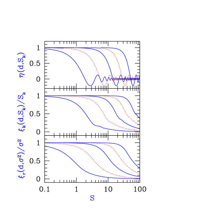
Figure 1: Various correlation functions. Upper panel:  each line shows $\eta(d,S_{k})$ as a function of $S_{k}$ for various values of $d$. From left to right $d=10$, 3.3, 1, 0.33, and $0.1h^{-1}\,{\rm Mpc}$ respectively. Center panel:  $\xi_{k}(d,S_{k})/S_{k}$ as a function of $S_{k}$ for the same Lagrangian distances as in the upper panel, again arranged from left to right. Bottom panel:  $\xi_{r}(d,\sigma^{2})/\sigma^{2}$ as a function of $\sigma^{2}$, again for the same distances arranged from left to right.

Just as we needed the real-space variance in the one-point case, many of the relevant two-point quantities discussed below depend on the correlation between two spatial filters centered about two points at a separation $d$. In this case, the standard expression is

$$\xi_{r}(d,r_{1},r_{2})\equiv\frac{1}{2\pi^{2}}\int_{0}^{\infty}k^{2}dk\frac{\sin(kd)}{kd}P(k)W(kr_{1})W(kr_{2})\ ,$$ (18)

where $r_{1}$ and $r_{2}$ are the radii of the two filters, and $W(x)$ is again the top-hat window function given by eq. (14). Unfortunately, simply substituting this quantity for $\xi_{k}$ in analogy with the usual one-point ansatz of substituting $\sigma^{2}$ for $S_{k}$ does not yield an acceptable approximation. This is because in the simple limit $d\rightarrow 0$, the correct one-point results [see eq. (43) below] are recovered only if $\xi\rightarrow{\rm min}[\sigma^{2}(r_{1}),\sigma^{2}(r_{2})]$. In this work, then, we instead make use of

$$\xi_{r_{max}}(d,r_{1},r_{2})\equiv\xi_{r}[d,{\rm max}(r_{1},r_{2}),{\rm max}(r_{1},r_{2})]\ ,$$ (19)

which is equal to $\xi_{r}$ when the two filters have equal radii.

We have also explored an alternative approach, in which we replace $\xi_{r}$ with $\xi_{k}(d,S_{k})$ as in eq. (15), but now choosing the integration limit $k$ to correspond to real-space filtering, so that $S_{k}(k)=\sigma^{2}(r).$ In this case we define

$$\xi_{k(r)}(d,r_{1},r_{2})\equiv\xi_{k}\{d,{\rm min}[\sigma^{2}(r_{1}),\sigma^{2}(r_{2})]\},$$ (20)

where $k$ is not proportional to $1/r$ but instead these quantities are only indirectly related, with $r$ determining $\sigma^{2}$ which in turn determines $k$. In this approach, the derivatives of $\xi_{k(r)}$ with respect to $r_{1}$ and $r_{2}$ can be expressed analytically in terms of $\eta$, reducing the overall computational load.

These alternative definitions of the correlation function are illustrated in Figure 1 in which we plot $\xi_{r}(d,\sigma^{2})/\sigma^{2}\equiv\xi_{r}[d,r(\sigma^{2}),r(\sigma^{2})]/\sigma^{2}$ and $\xi_{k}(d,S_{k})/S_{k}$ as functions of $\sigma^{2}$ and $S_{k}$ respectively. This parameterization allows for a direct comparison between $\xi_{k}$ and $\xi_{r}$, and shows that while these two correlation functions are rather similar, $\xi_{r}/\sigma^{2}$ is smooth while $\xi_{k}/S_{k}$ shows oscillations at intermediate scales. While these oscillations are small, we have found that they become more pronounced in some of the two-point quantities discussed below. Thus we choose in this paper to base our ansatz on the smoother quantity $\xi_{r_{max}}$, despite the fact that its derivative must be calculated numerically.

In Fig. 2 we examine how these quantities vary as a function of scale. In the upper panel of this figure, we plot $S_{k}$ and $\sigma^{2}$ as functions of $k^{-1}$ and $r$ respectively. Here we see that while both functions decrease monotonically with increasing length scale, $\sigma^{2}$ is somewhat greater than $S$ at all spatial values, such that roughly $S_{k}(1/r)\approx\sigma^{2}(2r).$ Thus it is more appropriate to compare $r$ to $2/k$ than $1/k$. In the lower two panels of this figure, we plot $\xi_{k}$ and $\xi_{r}$ as functions of Lagrangian distance for various values of $S_{k}$ and $\sigma^{2}$, respectively. Here again we find much the same behavior as in Figure 1, with $\xi_{k}/S_{k}$ and $\xi_{r}/\sigma^{2}$ approaching 1 at small $d$ values, and the points becoming uncorrelated at large distances. Note also that $\xi_{k}/S_{k}$ again contains small oscillations at intermediate distances.

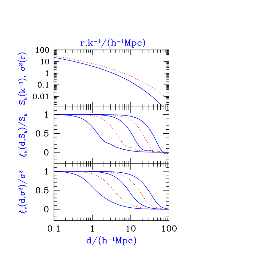
Figure 2: Variance and correlation functions as a function of scale. Upper panel:  The solid and dotted lines show $S_{k}(k^{-1})$ and $\sigma^{2}(r)$ respectively. Center panel:  $\xi_{k}(d,S_{k})/S_{k}$ as a function of $d$ for various values of $S_{k}$. From left to right $S_{k}$ = 10, 3.3, 1.0, 0.33, and 0.1, corresponding to $k^{-1}$ = 0.38, 1.3, 3.4, 6.8, and 12 comoving $h^{-1}\,{\rm Mpc}$ respectively. Bottom panel:  $\xi_{r}(d,\sigma^{2})/\sigma^{2}$ as a function of $d$. From left to right $\sigma^{2}$ = 10, 3.3, 1.0, 0.33, and 0.1, corresponding to $r$ = 0.70, 2.4, 6.5, 14, and 26 $h^{-1}\,{\rm Mpc}$.

3.2 Two Correlated Random Walks

With these correlation functions in hand, we now consider the simultaneous correlated random walks of two overdensities $\delta_{1}(S_{k,1})$ and $\delta_{2}(S_{k,2})$ separated by a fixed Lagrangian distance $d$. As in the one-point case, for the derivation we adopt sharp $k$-space filters. We want to determine the joint probability distribution of these two densities, $Q(\delta_{1},\delta_{2},S_{k,1},S_{k,2},d).$ In terms of a trajectory density in the $(\delta_{1},\delta_{2})$ plane, $Q(\delta_{1},\delta_{2},S_{k,1},S_{k,2},d)\,d\delta_{1}\,d\delta_{2}$ is the fraction of trajectories that are in the interval $\delta_{1}$ to $\delta_{1}+d\delta_{1}$ and $\delta_{2}$ to $\delta_{2}+d\delta_{2}$ at $(S_{k,1},S_{k,2})$. Below we will take $S_{k,1}$ and $S_{k,2}$ to be the final  variances of these trajectories, denoting intermediate variances with the primed notation $S^{\prime}_{k,1}$ and $S^{\prime}_{k,2}.$ We then consider a large number of random walks all of which begin with $\delta_{1}=0$ and $\delta_{2}=0$ at $S^{\prime}_{k,1}=0$ and $S^{\prime}_{k,2}=0$.

With sharp $k$-space filters, the problem simplifies due to the fact that we are working with a Gaussian random field. Suppose we consider random walks $\delta_{1}(S_{k,1}^{\prime})$ and $\delta_{2}(S_{k,2}^{\prime})$ over the ranges $0\leq S_{k,1}^{\prime}\leq S_{k,1}$ and $0\leq S_{k,2}^{\prime}\leq S_{k,2}$. Since different $k$-modes are independent of each other, any part of the random walk $\delta_{1}$, e.g., in the range $S_{k}<S_{k,1}^{\prime}<S_{k}+dS_{k}$, is only correlated with the same range, $S_{k}<S_{k,2}^{\prime}<S_{k}+dS_{k}$, in the other random walk, with a correlation strength determined by $\eta(d,S_{k})$. This means that in order to determine the joint probability distribution $Q(\delta_{1},\delta_{2},S_{k,1},S_{k,2},d)$, we do not need to vary $S_{k,1}^{\prime}$ and $S_{k,2}^{\prime}$ independently; instead we can consider $Q$ to be a function of a single variable $S^{\prime}_{k}$ (in addition to the variables $\delta_{1}$, $\delta_{2}$, and $d$). If the final $S^{\prime}_{k}$ values are unequal, e.g., $S_{k,1}>S_{k,2}$, then we continuously increase $S^{\prime}_{k}$ from 0 to $S_{k,2}$, generating the two correlated random walks and solving for $Q$ on the line $S^{\prime}_{k,1}=S^{\prime}_{k,2}=S^{\prime}_{k}$ in the $(S_{k,1},S_{k,2})$ plane, and we then continue to increase $S^{\prime}_{k}$ up to $S_{k,1}$, with only the random walk $\delta_{1}$ continuing further (with $S_{k,1}^{\prime}=S^{\prime}_{k}$).

We thus divide the evolution of $Q$ into two segments, one in which the $k$-space filter includes only small wavenumbers, such that $S^{\prime}_{k}$ is smaller than both $S_{k,1}$ and $S_{k,2}$, and a second segment of wavenumbers such that $S^{\prime}_{k}$ is between $S_{k,1}$ and $S_{k,2}$. With $d$ fixed, we follow the derivation from the one-point case and expand $Q(\delta_{1}-\Delta\delta_{1},\delta_{2}-\Delta\delta_{2},S^{\prime}_{k}-\Delta S^{\prime}_{k},d)$ to obtain

$$\Delta S^{\prime}_{k}\frac{\partial Q}{\partial S^{\prime}_{k}}=\frac{1}{2}\left\langle\Delta\delta_{1}^{2}\right\rangle\frac{\partial^{2}Q}{\partial\delta_{1}^{2}}+\left\langle\Delta\delta_{1}\Delta\delta_{2}\right\rangle\frac{\partial^{2}Q}{\partial\delta_{1}\delta_{2}}+\frac{1}{2}\left\langle\Delta\delta_{2}^{2}\right\rangle\frac{\partial^{2}Q}{\partial\delta_{2}^{2}}.$$ (21)

Evaluating the expectation values in each regime gives

$$\frac{\partial Q}{\partial S^{\prime}_{k}}=\cases{\frac{1}{2}\frac{\partial^{2}Q}{\partial\delta_{1}^{2}}+\eta(d,S^{\prime}_{k})\,\frac{\partial^{2}Q}{\partial\delta_{1}\delta_{2}}+\frac{1}{2}\frac{\partial^{2}Q}{\partial\delta_{2}^{2}}&$\ S^{\prime}_{k}<S_{k,1},S_{k,2}$\cr\frac{1}{2}\frac{\partial^{2}Q}{\partial\delta_{1}^{2}}&$\ S_{k,2}<S^{\prime}_{k}<S_{k,1}$\cr\frac{1}{2}\frac{\partial^{2}Q}{\partial\delta_{2}^{2}}&$\ S_{k,1}<S^{\prime}_{k}<S_{k,2}$\ .\cr}$$ (22)

In order to compute the evolution of these points in the regime in which $S^{\prime}_{k}<S_{k,1},S_{k,2}$ it is simpler to transform to the uncorrelated variables $\delta_{+}=(\delta_{1}+\delta_{2})/\sqrt{2}$ and $\delta_{-}=(\delta_{1}-\delta_{2})/\sqrt{2}$. In this case we obtain

$$\frac{\partial Q}{\partial S^{\prime}_{k}}=\frac{1+\eta}{2}\,\frac{\partial^{2}Q}{\partial\delta_{+}^{2}}+\frac{1-\eta}{2}\,\frac{\partial^{2}Q}{\partial\delta_{-}^{2}}\ .$$ (23)

In these variables the two random walks are independent, and the usual no-barrier solution is

$$Q_{0}(\delta_{+},\delta_{-},S_{k,{\rm min}},\xi_{k})=G[\delta_{+},S_{k,{\rm min}}+\xi_{k}]\,G[\delta_{-},S_{k,{\rm min}}-\xi_{k}]\ ,$$ (24)

where

$$S_{k,{\rm min}}\equiv{\rm min}(S_{k,1},S_{k,2})\ ,$$ (25)

and the covariance of $\delta_{1}$ and $\delta_{2}$ at $S_{k,{\rm min}}$ is $\xi_{k}\equiv\xi_{k}(d,S_{k,{\rm min}})$ [see eq. (17)]. The solution at the point $(S_{k,1},S_{k,2})$ is then simply obtained by convolving $Q_{0}(\delta_{+},\delta_{-},S_{k,{\rm min}},\xi_{k})$ with $G(\delta_{1},S_{k,1}-S_{k,2})$ or $G(\delta_{2},S_{k,2}-S_{k,1}).$

¿From eq. (24) we see that in the $\delta_{+}$ and $\delta_{-}$ coordinates, the evolution of the densities is particularly simple, and there are clearly image solutions of the form $Q_{0}(w_{+}-\delta_{+},w_{-}-\delta_{-},S_{k,{\rm min}},\xi_{k})$, where $w_{+}$ and $w_{-}$ are arbitrary constants. But unlike the one-dimensional case, the absorbing barriers at $\delta_{1}=\nu_{1}$ and $\delta_{2}=\nu_{2}$ are complicated due to the coordinate transformation, where, e.g., one of the barriers takes the form $\delta_{+}\,+\,\delta_{-}=w$, where $w$ is a constant. We want a solution for $Q$ which is zero on this barrier, but the image solutions do not help since $\delta_{+}$ and $\delta_{-}$ are coupled in the equations that describe the barriers. An exact solution thus requires a numerical approach, in which the diffusion equation is solved with the absorbing barrier imposed at each time step. However, in the following section we derive an accurate analytic approximation to the exact solution.

3.3 Two-Step Approximation

While the full solution of the double barrier problem requires a numerical approach, a closer look at the problem leads to a a simple approximate analytic solution that captures the underlying physics of two-point collapse. Note that we need only approximate the evolution for $0\leq S^{\prime}_{k}\leq S_{k,{\rm min}}$, since the evolution for higher values of $S^{\prime}_{k}$ involves only one of the random walks and therefore has a simple exact solution.

We consider the equation for the differential correlation function between the halos as a function of mass, eq. (16). While $\eta(d,S^{\prime}_{k})$ is an oscillating function, it equals unity at small values of $S_{k}$ and its amplitude steadily declines with $S^{\prime}_{k}$ as the corresponding wavenumber $k$ enters the regime in which $kr\gg 1$. Thus for small $S^{\prime}_{k}$ values, the two random walks are essentially identical, with $\delta_{1}(S^{\prime}_{k})\simeq\delta_{2}(S^{\prime}_{k})$. In this regime we can simply evolve a single random walk in $\delta_{1}$, and then set $\delta_{2}$ equal to the resulting final value of $\delta_{1}$. At large $S^{\prime}_{k}$, on the other hand, $\eta(d,S^{\prime}_{k})\rightarrow 0$, the two random walks become independent, and the problem again simplifies.

These observations lead us to propose a “two-step” approximation in which we replace $\eta(d,S^{\prime}_{k})$ with a simple step function that jumps from unity to zero at some value of $S^{\prime}_{k}$. We choose this jump to occur at a value of $S^{\prime}_{k}$ that preserves the exact solution for $Q$ at $S^{\prime}_{k}=S_{k,{\rm min}}$ in the absence of the barriers. In the no-barrier case, the joint distribution of $\delta_{1}$ and $\delta_{2}$ at $S_{k,{\rm min}}$ depends only on the variance $S_{k,{\rm min}}$ of each of these Gaussian variables, and on their covariance $\xi_{k}(d,S_{k,{\rm min}})$ which is given by eq. (17). In order for the integral in eq. (17) to be the same for both the exact function $\eta(d,S^{\prime}_{k})$ and for the step-function approximation, we must fix the step to occur at $S^{\prime}_{k}=\xi_{k}(d,S_{k,{\rm min}})$. Thus, our two-step approximation is

$$\eta(d,S^{\prime}_{k})\simeq\cases{1&$0\leq S^{\prime}_{k}\leq\xi_{k}(d,S_{k,{\rm min}})$\cr 0&$\xi_{k}(d,S_{k,{\rm min}})<S^{\prime}_{k}\leq S_{k,\rm min}$\ ,\cr}$$ (26)

such that the trajectories are completely correlated when $S^{\prime}_{k}$ is less than the cross-correlation between the points at $S_{k,{\rm min}}$, and completely uncorrelated when $S^{\prime}_{k}$ exceeds this value. This approximation is compared to the exact form of $\eta(d,S^{\prime}_{k})$ for various values of $S^{\prime}_{k}$ in Fig. 3.

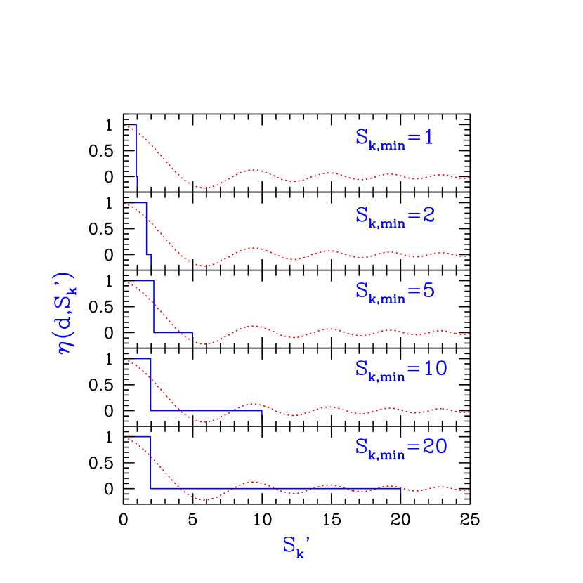
Figure 3: Comparison between $\eta(d,S^{\prime}_{k})$ calculated exactly (solid lines) and in the two-step approximation (dotted lines), for various values of $S_{k,{\rm min}}$. In all plots $d=3.3$ comoving $h^{-1}\,{\rm Mpc}$.

We combine this approximation for the evolution of the two random walks for $S^{\prime}_{k}\leq S_{k,{\rm min}}$ with the single random walk which continues for $S^{\prime}_{k}>S_{k,{\rm min}}$, resulting in the following overall prescription with absorbing barriers at $\delta_{1}=\nu_{1}$ and $\delta_{2}=\nu_{2}$. First, we evolve $\delta_{1}$ for $0\leq S^{\prime}_{k}\leq\xi_{k}(d,S_{k,{\rm min}})$. Since we are assuming that the two random walks are identical in this regime, we must place the barrier on $\delta_{1}$ at

$$\nu_{\rm min}\equiv{\rm min}(\nu_{1},\nu_{2})\ .$$ (27)

Quantitatively, the single absorbing barrier solution, eq. (8), gives $Q$ at $S^{\prime}_{k}=\xi_{k}(d,S_{k,{\rm min}})$,

$$Q_{a}(\nu_{\rm min},\delta_{1},\delta_{2},\xi_{k})=[G(\delta_{1},\xi_{k})-G(2\nu_{\rm min}-\delta_{1},\xi_{k})]\,\delta_{D}(\delta_{1}-\delta_{2})\theta(\nu_{\rm min}-\delta_{1}),$$ (28)

where $\delta_{D}$ is a one-dimensional Dirac delta function, $\theta$ is the Heaviside step function, and here and in the rest of this section $\xi_{k}$ refers to $\xi_{k}(d,S_{k,{\rm min}})$. We then set $\delta_{2}=\delta_{1}$ and evolve the random walks in $\delta_{1}$ and $\delta_{2}$ independently up to $S_{k,1}$ and $S_{k,2}$, with the barriers at $\nu_{1}$ and $\nu_{2}$, respectively. Thus, we first convolve eq. (28) with the no-barrier solutions for the two independent random walks,

$$Q_{b}(\delta_{1},\delta_{2},S_{k,1},S_{k,2},\xi_{k})=G(\delta_{1},S_{k,1}-\xi_{k})\,G(\delta_{2},S_{k,2}-\xi_{k})\ ,$$ (29)

which gives

$$Q_{0}(\nu_{\rm min},\delta_{1},\delta_{2},S_{k,1},S_{k,2},\xi_{k}) = Q_{+}(\nu_{\rm min},\delta_{1},\delta_{2},S_{k,1},S_{k,2},\xi_{k})\ +$$ (30)

$$Q_{-}(\nu_{\rm min},2\nu_{\rm min}-\delta_{1},2\nu_{\rm min}-\delta_{2},S_{k,1},S_{k,2},\xi_{k})\ ,$$

where

$$Q_{\pm}(\nu_{\rm min},\delta_{1},\delta_{2},S_{k,1},S_{k,2},\xi_{k}) \equiv \frac{1}{4\pi\sqrt{S_{k,1}S_{k,2}-\xi_{k}^{2}}}\,\exp\left[-\,\frac{\delta_{1}^{2}S_{k,2}+\delta_{2}^{2}S_{k,1}-2\delta_{1}\delta_{2}\xi_{k}}{2(S_{k,1}S_{k,2}-\xi_{k}^{2})}\right]$$ (31)

$$\times\left[{\rm erf}\left(\tilde{\nu}\sqrt{\frac{\tilde{S}}{2}}\right)\pm 1\right],$$

and

$$\tilde{S}\equiv\frac{\xi_{k}(S_{k,1}-\xi_{k})(S_{k,2}-\xi_{k})}{S_{k,1}S_{k,2}-\xi_{k}^{2}}\ ,\qquad\qquad\tilde{\nu}\equiv\ \frac{\nu_{\rm min}}{\tilde{S}}-\frac{\delta_{1}}{S_{k,1}-\xi_{k}}-\frac{\delta_{2}}{S_{k,2}-\xi_{k}}\ .$$ (32)

Finally, we account for the additional barriers with reflections about the $\nu_{1}$ and $\nu_{2}$ axes, which yields

$$Q(\nu_{1},\nu_{2},\delta_{1},\delta_{2},S_{k,1},S_{k,2},\xi_{k}) = Q_{0}(\nu_{\rm min},\delta_{1},\delta_{2},S_{k,1},S_{k,2},\xi_{k})\ +$$ (33)

$$Q_{0}(\nu_{\rm min},2\nu_{1}-\delta_{1},2\nu_{2}-\delta_{2},S_{k,1},S_{k,2},\xi_{k})\ -$$

$$Q_{0}(\nu_{\rm min},\delta_{1},2\nu_{2}-\delta_{2},S_{k,1},S_{k,2},\xi_{k})\ -$$

$$Q_{0}(\nu_{\rm min},2\nu_{1}-\delta_{1},\delta_{2},S_{k,1},S_{k,2},\xi_{k})\ .$$

Following the common approximation taken in the single particle case we again replace $S_{k,1}$ and $S_{k,2}$ with $\sigma^{2}(M_{1})$ and $\sigma^{2}(M_{2})$, respectively. Similarly, we also replace $\xi_{k}$ with the correlation function of real-space peaks $\xi_{r_{max}}$ as given by eq. (19). Using this expression we can now construct the combined mass function of halos at two points separated by a comoving Lagrangian distance $d$. Before we derive this function, however, it is important to understand the errors introduced by our simple two-step approach. Thus, we compare eq. (33) with exact numerical solutions in order to show that our analytic approximation is accurate over a broad range of parameter space.

3.4 Numerical Approach and Comparison with Two-Step Approximation

In order to solve eq. (23) in the presence of absorbing barriers at fixed values of $\delta_{1}$ and $\delta_{2}$ we have developed a simple finite difference code. We construct a 400 $\times$ 400 zone mesh in $\delta_{+}$ and $\delta_{-}$ spanning the range from $-5\,\delta_{\rm scale}\leq\delta_{+}\leq 5\,\delta_{\rm scale}$ and $-5\,\delta_{\rm scale}\leq\delta_{-}\leq 5\,\delta_{\rm scale}$, where $\delta_{\rm scale}$ is a typical overdensity of interest. In this case the width of each zone, $dx$, is $0.025\,\delta_{\rm scale}$ in both dimensions. On this grid, we construct $Q_{i,j}^{t}=Q(\delta_{+,i},\delta_{-,j},S^{\prime}_{k}(t))$ where $i$ and $j$ are spatial indices in each of directions and $t$ is a “time” counter such that $S^{\prime}_{k}(t)=t\,dS^{\prime}_{k},$ where we take $dS^{\prime}_{k}=\delta_{\rm scale}^{2}/3000$ to be the interval by which we refine our $k$-space filter at each time step.

Initially the distribution is taken to be a delta function, such that $Q^{0}_{0,0}=1$ and $Q^{0}_{i,j}=0$ for all other values of $i$ and $j$. We calculate the values at each new step in $S^{\prime}_{k}$ using an alternating-direction implicit method (Press et al., 1992) in which we divide each time step into two stages of size $dS^{\prime}_{k}/2$, and solve first in the $x$ and then the $y$ direction. In this case eq. (23) becomes

$$Q^{t+1/2}_{i,j} = Q^{t}_{i,j}+\frac{\alpha_{+}}{2}\left[Q^{t+1/2}_{i-1,j}-2Q^{t+1/2}_{i,j}+Q^{t+1/2}_{i+1,j}\right]+\frac{\alpha_{-}}{2}\left[Q^{t}_{i,j-1}-2Q^{t}_{i,j}+Q^{t}_{i,j+1}\right],$$

$$Q^{t+1}_{i,j} = Q^{t+1/2}_{i,j}+\frac{\alpha_{+}}{2}\left[Q^{t+1/2}_{i-1,j}-2Q^{t+1/2}_{i,j}+Q^{t+1/2}_{i+1,j}\right]+\frac{\alpha_{-}}{2}\left[Q^{t+1}_{i,j-1}-2Q^{t+1}_{i,j}+Q^{t+1}_{i,j+1}\right],$$ (34)

where $\alpha_{+}\equiv\frac{[1+\eta(d,S^{\prime}_{k})]dS^{\prime}_{k}}{2\,dx^{2}}$, $\alpha_{-}\equiv\frac{[1-\eta(d,S^{\prime}_{k})]dS^{\prime}_{k}}{2\,dx^{2}}$, and the system can be solved using simple inversions of tridiagonal matrices. Finally, at the end of each time step we impose the absorbing barriers at $\delta_{1}=\nu_{1}$ and $\delta_{2}=\nu_{2}$ by setting $Q_{i,j}^{t+1,n}=0$ at all points at which $\delta_{+,i}+\delta_{-,j}\geq\sqrt{2}\,\nu_{1}$ or $\delta_{+,i}-\delta_{-,j}\geq\sqrt{2}\,\nu_{2}.$ With this code we are able to examine the accuracy of our two-step approximation for a number of physical cases.

For any given redshifts $z_{1}$ and $z_{2}$, we fix the barriers at the collapse thresholds $\nu_{1}=\delta_{c}(z_{1})$ and $\nu_{2}=\delta_{c}(z_{2})$, and consider the following quantity:

$$F(\nu_{1},\nu_{2},S_{k,1},S_{k,2},\xi_{k})=\int_{-\infty}^{\nu_{1}}d\delta_{1}\int_{-\infty}^{\nu_{2}}d\delta_{2}\,Q(\nu_{1},\nu_{2},\delta_{1},\delta_{2},S_{k,1},S_{k,2},\xi_{k})\ .$$ (35)

This is the fraction of trajectories that are not absorbed before the random walks reach the point $(S_{k,1},S_{k,2})$. Recall that $S_{k}$ can be related to the mass scale of the collapsed objects by the simple ansatz $S_{k}\rightarrow\sigma^{2}(r)$ as described in §3.1 Thus equation eq. (35) can be interpreted as the probability of point $A$ being in a halo of mass $M<M_{1}(\sigma^{2}=S_{k,1})$ and point $B$ in a halo of mass $M<M_{2}(\sigma^{2}=S_{k,2})$. Since $F$ is the basic quantity that we later use to calculate various halo properties, a reasonable way to judge the success of our approximate method is to test its ability to closely reproduce this function. In the comparisons (Figures 4 and 5), we use the $k$-filter quantities $S_{k}$ and $\xi_{k}$.

In Figure 4 we compare analytical and numerical values of $F(\nu_{1},\nu_{2},S_{k,1},S_{k,2},\xi_{k})$ as a function of $S_{k,1}=S_{k,2}=S$ for various distances and collapse redshifts. In the left three panels of this figure, we consider large objects collapsing at different redshifts by fixing $\nu_{1}=4.13=\delta_{c}(z_{1}=2)$, $\nu_{1}=5.47=\delta_{c}(z_{2}=3)$, $\delta_{\rm scale}=3.0$ and varying the distances as labeled. In the right panels we consider the simultaneous collapse of somewhat smaller objects at earlier times fixing $\nu_{1}=\nu_{2}=12.35=\delta_{c}(z=8)$ and $\delta_{\rm scale}=8.0$. The figure shows that both for peaks that form simultaneously, and for peaks that collapse at different times, the two-step solution tracks the numerical solution over a large range of halo masses and distances. Note also that these expressions match each other closely even when they are very different from both the correlated and the uncorrelated cases.

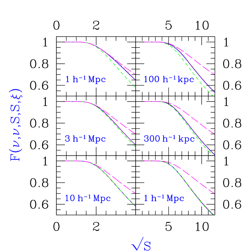
Figure 4: Comparison between numerical solution and two-step approximation as a function of $S$. In the left panels we consider two peaks that collapse at redshifts 2 and 3, respectively, while in the right panels we consider two peaks that collapse at $z=8$. The panels are labeled by the comoving Lagrangian distance between the peaks, and in each panel the numerical solution and the two-step solution are given by the solid and dotted line, respectively, while for comparison, the fully uncorrelated solution is given by the short-dashed line and the fully correlated solution is given by the long-dashed line. Note that the two-step approximation is almost indistinguishable from the numerical solution, in every panel. Note also that in this plot we use $S_{k}$ for $S$ and $\xi_{k}$ for $\xi$.

In Figure 5 we fix three values of $S_{k,1}=S_{k,2}=S$ and the collapse redshift of a single halo $z_{1}=5$, and consider $F$ as a function of the collapse redshift $z_{2}$ of the second halo, at three different separations. The figure shows that our approximation does well at reproducing the numerical results even for cases in which the collapse redshifts between the two objects are very different. As before, the numerical and approximate results are in good agreement over a wide range of values for which the fully-correlated and fully-uncorrelated expressions are not accurate.

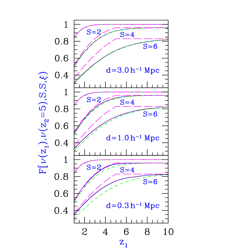
Figure 5: Comparison between numerical solution and two-step approximation as a function of $z_{2}$. The panels are again labeled by the comoving Lagrangian distance between the peaks, and in each panel the numerical solution and two-step solutions are given by the solid and dotted line, respectively, and the fully uncorrelated and fully correlated solutions are given by the short-dashed and long-dashed line, respectively. All four lines coincide for $S=2$. For $S=4$ and $S=6$, our approximation and the numerical calculation are almost indistinguishable, but the uncorrelated and the fully correlated lines lie significantly lower and higher, respectively. Note that in this plot we use $S_{k}$ for $S$ and $\xi_{k}$ for $\xi$.

Besides the results shown in these figures, we have conducted extensive convergence tests varying $dS$ and $dx$, and have found that reducing any of these parameters has no effect on our numerical results. Thus we are confident that the differences between the analytic and exact solutions, as presented in Figures 4 and 5, are in general small, and the errors in our analytical expressions are at most $2\%.$

4 Structure Formation with the Two-Point Formalism

4.1 Bivariate Mass Function

Having developed in the previous section an accurate approximation to the joint probability distribution at two points, we now apply this distribution to derive the two-point generalization of the Press-Schechter mass function of collapsed halos. This generalization is the joint probability of having point $A$ lie in a halo in the mass range $M_{1}$ to $M_{1}+dM_{1}$ at a redshift $z_{1}$ and point $B$ lie in a halo in the mass range $M_{2}$ to $M_{2}+dM_{2}$ at a redshift $z_{2}$. Note that the derivation in $\S 3.2$ applies to any redshifts $z_{1}$ and $z_{2}$ and thus our calculation can determine the number density of halos at $B$ both before and after the formation of a halo at $A$.

Again, it is important to emphasize that this joint mass function is defined in the Lagrangian coordinate system that arises naturally in an excursion-set approach. Thus the distance between the points in physical space may be somewhat different than the $d$ considered in our equations, as the relevant comoving distance in our case is that separating the points at early times. This coordinate system has both its weaknesses and its advantages. While it somewhat complicates the direct comparison of our expressions with numerical simulations, this can in general be remedied with estimates of the final, Eulerian halo coordinates (e.g., Mo & White, 1996). Furthermore, for many applications, Lagrangian results are in fact preferable to an Eulerian description in which halos are indexed by their physical coordinates with no reference to where these perturbations came from. In studies of spatially-dependent feedback in structure formation, for example, it is often more important to have a measure of the total column depth of material separating two perturbations than their precise distance in physical space.

In this section, we adopt a general notation for the variances and correlation functions, using $S$ to represent either the $k$-space filtered quantity, $S_{k}$, its real space equivalent $\sigma^{2}(r)$, or any alternative definition. Similarly, $\xi$ denotes $\xi_{r_{max}}$, $\xi_{k(r)}$, or any alternative definition of the correlation function. With this notation, we now consider $f(\nu_{1},\nu_{2},S_{1},S_{2},\xi)\,dS_{1}\,dS_{2}$, the probability of having point $A$ in a halo with mass corresponding to the range $S_{1}$ to $S_{1}+dS_{1}$ and point $B$ in a halo with mass corresponding to the range $S_{2}$ to $S_{2}+dS_{2}$. This is simply related to the quantity in eq. (35) as

$$f(\nu_{1},\nu_{2},S_{1},S_{2},\xi)=\frac{\partial}{\partial S_{1}}\frac{\partial}{\partial S_{2}}\int_{-\infty}^{\nu_{1}}d\delta_{1}\int_{-\infty}^{\nu_{2}}d\delta_{2}\,Q(\nu_{1},\nu_{2},\delta_{1},\delta_{2},S_{1},S_{2},\xi)\ ,$$ (36)

where $\xi$ is not considered an independent variable (and so the partial derivatives involve variations of $\xi$). This simplifies to

$$f(S_{1},S_{2},\nu_{1},\nu_{2},\xi)=\frac{\partial}{\partial S_{1}}\frac{\partial}{\partial S_{2}}\left[2\int_{-\infty}^{\nu_{1}}d\delta_{1}-\int_{-\infty}^{\infty}d\delta_{1}\right]\left[2\int_{-\infty}^{\nu_{2}}d\delta_{2}-\int_{-\infty}^{\infty}d\delta_{2}\right]Q_{0}(\nu_{1},\nu_{2},\delta_{1},\delta_{2},S_{1},S_{2},\xi)\ .$$ (37)

In order to perform these integrals, we must consider $Q_{0}$ from eq. (30) in its unintegrated form, written as a convolution with an integration variable $x$:

$$Q_{0}=\int_{-\infty}^{\nu_{\rm min}}dx\,\left[G(x,\xi)-G(2\nu_{\rm min}-x,\xi)\right]\,G(\delta_{1}-x,S_{1}-\xi)\,G(\delta_{2}-x,S_{2}-\xi)\ .$$ (38)

Since $S_{1}$ and $\delta_{1}$ appear only in a single term in the $x$-integration, and similarly for $S_{2}$ and $\delta_{2}$, $Q_{0}$ satisfies

$$\frac{\partial Q_{0}}{\partial S_{1}}=\frac{1}{2}\frac{\partial^{2}Q_{0}}{\partial\delta_{1}^{2}}+\frac{\partial\xi}{\partial S_{1}}\frac{\partial Q_{0}}{\partial\xi}\ ,\qquad{\rm and}\qquad\frac{\partial Q_{0}}{\partial S_{2}}=\frac{1}{2}\frac{\partial^{2}Q_{0}}{\partial\delta_{2}^{2}}+\frac{\partial\xi}{\partial S_{2}}\frac{\partial Q_{0}}{\partial\xi}\ ,$$ (39)

where we consider $\xi$ to be an independent variable when calculating $\frac{\partial Q_{0}}{\partial\xi}.$

We perform the partial derivatives with respect to $S_{1}$ and $S_{2}$ on the integrand in equation (38), obtaining four terms. Terms that contain partial derivatives with respect to $\delta_{1}$ or $\delta_{2}$ allow us to perform the $\delta_{1}$ or $\delta_{2}$ integrations in eq. (37) trivially, while the evaluation of terms containing $\frac{\partial Q_{0}}{\partial\xi}$ is more involved.

To compute $\frac{\partial Q_{0}}{\partial\xi}$, we note that the integrand in eq. (38) is a product of three terms, which we denote, respectively from left to right, as $I_{1}$, $I_{2}$, and $I_{3}$. These satisfy the equations

$$\frac{\partial I_{1}}{\partial\xi}=\frac{1}{2}\frac{\partial^{2}I_{1}}{\partial x^{2}}\ ,\qquad{\rm and}\qquad\frac{\partial I_{2,3}}{\partial\xi}=-\frac{1}{2}\frac{\partial^{2}I_{2,3}}{\partial x^{2}},$$ (40)

which allow us to perform the integration with respect to $x$, using integration by parts to eliminate all double derivatives. This yields an integrated term, whose contribution to $f(\nu_{1},\nu_{2},S_{1},S_{2},\xi)$ is zero, and the remaining term in $\frac{\partial Q_{0}}{\partial\xi}$ is

$$\int_{-\infty}^{\nu_{\rm min}}dx\,I_{1}\,\partial_{x}I_{2}\,\partial_{x}I_{3}\ .$$

Finally we use $\partial_{x}I_{2}=-\partial_{\delta_{1}}I_{2}$ and $\partial_{x}I_{3}=-\partial_{\delta_{2}}I_{3}$ to further simplify any term that contains a partial derivative with respect to $\xi$, yielding

$$f(\nu_{1},\nu_{2},S_{1},S_{2},\xi)=\left.\left[\frac{\partial^{2}Q_{0}}{\partial\delta_{1}\partial\delta_{2}}+\,2\left(\frac{\partial\xi}{\partial S_{1}}\,\frac{\partial^{2}Q_{0}}{\partial\delta_{2}^{2}}+\frac{\partial\xi}{\partial S_{2}}\,\frac{\partial^{2}Q_{0}}{\partial\delta_{1}^{2}}\right)+4\left(\frac{\partial\xi}{\partial S_{1}}\frac{\partial\xi}{\partial S_{2}}\frac{\partial Q_{0}}{\partial\xi}+\frac{\partial^{2}\xi}{\partial S_{1}\partial S_{2}}\,Q_{0}\right)\right]\right|_{\delta_{1}=\nu_{1},\,\delta_{2}=\nu_{2}}\ .$$ (41)

Note that this expression is discontinuous for some choices of $S$ and $\xi$. This is true both for the $k$-space-filtering case for which eqs. (31) and (33) were derived, as well as the real-space case in which $\xi=\xi_{r_{max}}$ and $S=\sigma^{2}$, because in each case $\xi$ is a function of $S_{\rm min}$ whose derivatives with respect to $S_{1}$ and $S_{2}$ are not continuous. While this may seem at first to be a serious problem, a closer look at these discontinuities shows that they are in fact quite harmless.

To see why this is true, consider the case in which $S_{1}$ and $S_{2}$ are nearly equal. If $S_{1}=S_{2}-\epsilon$, then only the $\frac{\partial^{2}Q_{0}}{\partial\delta_{1}\partial\delta_{2}}$ and $\frac{\partial^{2}Q_{0}}{\partial\delta_{2}^{2}}$ terms of eq. (41) are nonzero (since in this case $\xi$ is a function of $S_{\rm min}=S_{1}$), while if $S_{1}=S_{2}+\epsilon$ then the only nonzero terms are the mixed derivative term and $\frac{\partial^{2}Q_{0}}{\partial\delta_{1}^{2}}$. Now, in the limited case in which $\nu_{1}=\nu_{2}$, $\frac{\partial^{2}Q_{0}}{\partial\delta_{1}^{2}}$ and $\frac{\partial^{2}Q_{0}}{\partial\delta_{2}^{2}}$ are equal at $S_{1}=S_{2}$ and $f$ is continuous at this point, while if $\nu_{1}\neq\nu_{2}$, $f$ is discontinuous at $S_{1}=S_{2}$.

This discontinuity at $\nu_{1}\neq\nu_{2}$ is not a limitation of our method, however, but is instead a true reflection of the physical situation. This is clearest in the $d=0$ case in which the two points coincide. In this case, if $\nu_{1}<\nu_{2}$ and thus $z_{1}<z_{2}$, taking $S_{1}=S_{2}-\epsilon$ corresponds to $M_{1}>M_{2}$ which is simply the accretion of mass over time. Taking $S_{1}=S_{2}+\epsilon,$ however, would correspond to losing  mass with time, which is contradictory to our most basic assumptions. Thus, approaching $S_{1}=S_{2}$ from different directions has two different meanings, only one of which is relevant to structure formation. The problem therefore arises from defining an effective arrow of time and considering only the first-crossing distribution with respect to it. Thus, the discontinuity only occurs in transitions between physically relevant choices of parameters and regions of parameter space that contradict the whole premise of our approach, and it need not concern us.

In Appendix A we give all the expressions necessary to evaluate eq. (41) explicitly. We can thus analytically compute the joint halo abundance as

$$\frac{d^{2}n^{2}_{12}}{dM_{1}dM_{2}}=\frac{\bar{\rho}}{M_{1}}\left|\frac{dS_{1}}{dM_{1}}\right|\frac{\bar{\rho}}{M_{2}}\left|\frac{dS_{2}}{dM_{2}}\right|f(\nu_{1},\nu_{2},S_{1},S_{2},\xi)\ ,$$ (42)

which reduces to the product of $\frac{dn_{1}}{dM_{1}}$ and $\frac{dn_{2}}{dM_{2}}$ as given by eq. (11) in the limit of large distances, when $\xi\rightarrow 0$. Note that the last two terms in eq. (41) are identically zero if we use $\xi_{k}$ or $\xi_{r_{max}}$ as our definition of $\xi$.

In Figure 6 we plot the normalized mass function, setting $S_{1}=\sigma^{2}(M_{1})$, $S_{2}=\sigma^{2}(M_{2})$, $\xi=\xi_{r_{max}}(d,M_{1},M_{2})$, and fixing $\nu_{1}=\nu_{2}=\delta_{c}(z)$ for various redshifts, in the same $\Lambda$CDM cosmology considered in §3. Each function is normalized by its uncorrelated value in order to emphasize the features of the joint distribution, i.e., each panel shows $\frac{d^{2}n^{2}_{12}}{dM_{1}dM_{2}}\left[\frac{dn_{1}}{dM_{1}}\times\frac{dn_{2}}{dM_{2}}\right]^{-1}$ as a function of $M_{2}$, for various values of $d$, $M_{1}$, and $z$.

In the left panels of this figure we fix $M_{1}$ to be $10^{12}h^{-1}\,M_{\odot}$, corresponding to a typical $L_{\star}$ galaxy, and construct the normalized number density at redshifts $1$ and $2$, and Lagrangian distances of $d=1$, 3.3, and 10 comoving $h^{-1}\,{\rm Mpc}$. At the larger distances, the presence of a perturbation at point $A$ enhances the formation of an object at point $B$, unless $M_{2}$ is so large that such a halo at point $B$ would very likely absorb point $A$ into it as well. Thus the $d$ = 3.3 and 10 comoving $h^{-1}\,{\rm Mpc}$ curves are enhanced at all but the largest $M_{2}$ values. This enhancement is more significant at $z=2$ as these peaks are rarer, and hence more highly biased.

As the points get closer, however ($d=1h^{-1}\,{\rm Mpc}$), the lines become strongly peaked at $M_{2}=M_{1}$, excluding the formation of objects of vastly different sizes at a short distance. Indeed, as $d\rightarrow 0$, $f$ approaches the single point differential mass function times a delta function, as both points must belong to the same peak in the limit when the two points become identical. Real applications of these results at short distances must consider more explicitly the issue of halo exclusion, i.e., the fact that a given halo at point $A$ contains all the mass from some region, and this halo either contains the point $B$ or not. More generally, the two regimes $M_{2}<M_{1}$ and $M_{2}>M_{1}$ should be considered separately because of their different physical interpretations (especially when $d$ is small); in the first case, $M_{2}$ is a small halo that may be accreted by $M_{1}$, and in the second case, $M_{2}$ is a large halo that may be about to absorb $M_{1}$ into it.

In the right panels, we consider the case of a dwarf galaxy with $M_{1}=10^{9}h^{-1}\,M_{\odot}$, forming at redshifts $z=4$ and $z=6$, such that $\nu(z)/\sigma(M_{1})$ and $\nu(z)/\sigma(M_{2})$ cover a similar range of values as in the $L_{\star}$-galaxy case. As the virial radii of these systems are smaller by a factor of 10, in these panels we fix $d$ = 0.1, 0.33, and 1.0 comoving $h^{-1}\,{\rm Mpc}$. These plots display essentially the same features as in the more massive case, although the effects of the correlations are somewhat larger since the objects are slightly rarer.

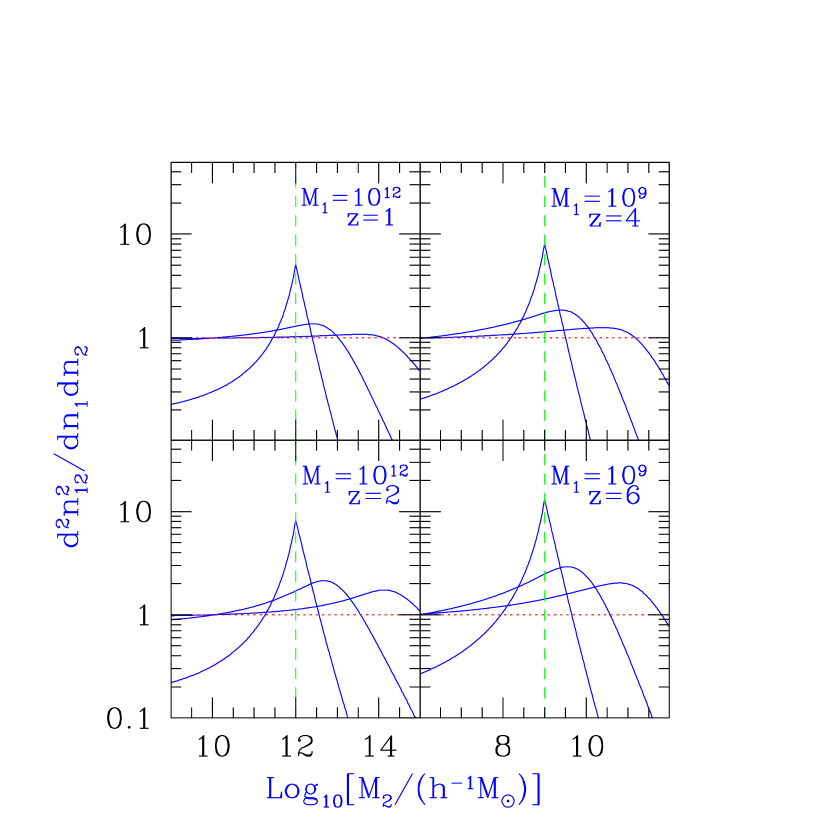
Figure 6: Normalized number density of correlated halos as calculated from eq. (42) as a function of $M_{2}$, for various values of distance, $M_{1}$, and redshift. In the left panels $M_{1}$ is held fixed at a value of $10^{12}h^{-1}\,M_{\odot}$, roughly corresponding to an $L_{\star}$ galaxy, at redshifts of 1 and 2. Here the solid lines show, from top to bottom (in terms of the highest point in each curve), results with the Lagrangian distances between the two points fixed at 1.0, 3.3, and 10 comoving $h^{-1}\,{\rm Mpc}$ respectively, while for reference the uncorrelated case is plotted as the dotted line at 1 and the mass at which $M_{1}=M_{2}$ is given by the vertical dashed line. In the right panels, we fix $M_{1}$ at $10^{9}h^{-1}\,M_{\odot}$ corresponding to a dwarf galaxy. Here we consider a higher range of redshift values ($z_{1}=z_{2}=4$ and $z_{1}=z_{2}=6$) roughly corresponding to the same values of $\nu/\sigma$ used in the $M_{1}=10^{12}h^{-1}\,M_{\odot}$ case. In these panels the solid lines show normalized densities at $d$ = 0.1, 0.33, and 1.0 comoving $h^{-1}\,{\rm Mpc}$, from top to bottom.

In Figure 7 we again plot the normalized number density of two points forming at the same redshift, but now holding $M_{2}$ fixed and varying the distance between the two perturbations. Here we see that as the points come closer to each other, the number densities are initially enhanced, as the collapse of an overdensity at the first point makes it likely that a large-scale overdensity enhances halo formation at all nearby points. As the perturbations are drawn closer together, the curves drop sharply if $M_{1}\neq M_{2}$ as it is impossible for two perturbations of different sizes to form at the same position and redshift. If $M_{1}=M_{2}$ however, the probability continues to rise dramatically at small distances, as $f$ approaches the single point differential mass function multiplied by a delta function. Again these effects are stronger at higher redshifts, as rare peaks are more highly correlated.

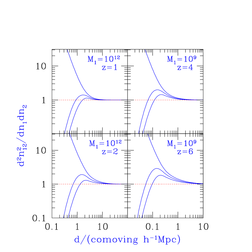
Figure 7: Normalized number density of correlated halos as calculated from eq. (42) as a function of $d$, for various values of $M_{1}$, $M_{2}$, and redshift. Again in the left panels $M_{1}$ is held fixed at a value of $10^{12}h^{-1}\,M_{\odot}$ at redshifts of 1 and 2, while the solid lines show, from top to bottom (in terms of the highest point in each curve), densities with $M_{2}$ fixed at $10^{12}h^{-1}\,M_{\odot}$, $3.3\times 10^{11}h^{-1}\,M_{\odot}$ and $10^{11}h^{-1}\,M_{\odot}$, respectively, and again the uncorrelated case is plotted as a dotted line at 1. Similarly, in the right panels, we fix $M_{1}$ to be $10^{9}h^{-1}\,M_{\odot}$ at redshifts 4 and 6. In these panels the solid lines show normalized densities at $M_{2}$ = $10^{9}h^{-1}\,M_{\odot}$, $3.3\times 10^{8}h^{-1}\,M_{\odot}$, and $10^{8}h^{-1}\,M_{\odot}$, from top to bottom.

Our formalism is not restricted to the collapse of two points at the same redshift, but is also well suited to study the formation of halos at varying times. In Figures 8 and 9 we again examine the formation at $z=1$ of an $M_{1}=10^{12}h^{-1}\,M_{\odot}$ halo associated with an $L_{\star}$ galaxy, and the formation at $z_{1}=4$ of an $M_{1}=10^{9}h^{-1}\,M_{\odot}$ halo associated with a dwarf galaxy. We now consider $M_{2}$ to be a smaller halo, formed at a distance $d$ and at an earlier redshift. This is essentially a generalization of the usual progenitor problem, where now the lower mass halo need not be absorbed into the larger halo, but can be located an arbitrary distance away.

In Figure 8 we consider the normalized number density as a function of $M_{2}$ for a variety of distances, fixing $z_{1}=1$ and $z_{2}=2$ and 4 in the $M_{1}=10^{12}h^{-1}\,M_{\odot}$ case shown in the left panels, and fixing $z_{1}=4$ and $z_{2}=6$ and 10 in the $M_{1}=10^{9}h^{-1}\,M_{\odot}$ case shown in the right panels. Many features in this plot parallel the $z_{1}=z_{2}$ cases: at the larger distances, the curves are enhanced at most $M_{2}$ values, as a second galaxy is likely to form near the first; and if the objects are too close together and have masses that are very different then they can suppress each other’s likelihood of formation.

Unlike the simultaneously collapsing cases, when $M_{1}=M_{2}$, $f$ does not approach a delta function as $d\rightarrow 0$. Instead, the formation of objects of equal mass at both points is completely excluded, as this would correspond to the same halo forming in the same place at two different times (while the formalism assumes continuous mass accretion for every halo). Each curve is instead peaked at an $M_{2}$ value that is smaller  than $M_{1}$, as this value roughly corresponds to the most likely progenitor at a redshift $z_{2}$ for the larger halo, which forms at $z_{1}$. These curves can be compared to the number densities expected for a progenitor at the same point (i.e., at $d=0$), first derived by Bond et al. (1991),

$$\frac{\nu_{2}-\nu_{1}}{\sqrt{2\pi}(S_{2}-S_{1})^{3/2}}\exp\left[-\frac{(\nu_{2}-\nu_{1})^{2}}{2(S_{2}-S_{1})}\right]\frac{\nu_{1}}{\sqrt{2\pi}S_{1}^{3/2}}\exp\left[-\frac{\nu_{1}^{2}}{2S_{1}}\right],$$ (43)

which is shown by the dashed lines. Note that as $d\rightarrow 0$, $f$ approaches this expression exactly.

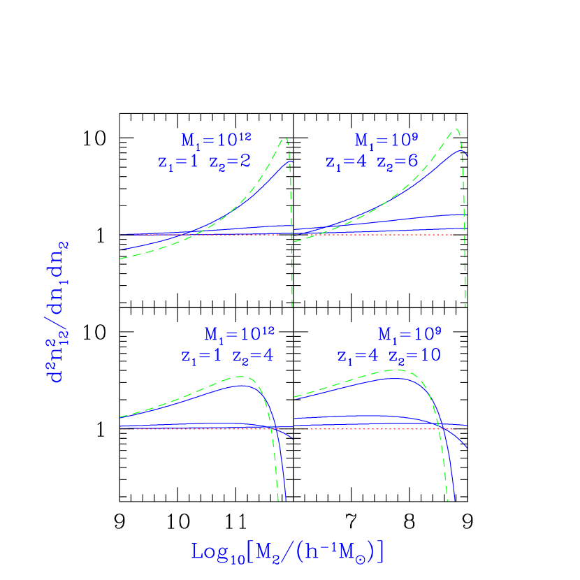
Figure 8: Normalized number density of halos as a function of $M_{2}$ for two objects forming at different redshifts. In the left panels, we fix $M_{1}=10^{12}h^{-1}\,M_{\odot}$ and $z_{1}=1$, and consider the second object as a generalized progenitor, forming at a higher redshift at a point nearby. In these panels, each of the solid lines correspond, from top to bottom (in terms of the highest point in each curve), to $d$ values $1$, $3.3$, and $10$ comoving $h^{-1}\,{\rm Mpc}$, and we consider cases in which $z_{2}=2$ and $z_{2}=4.$ In the right panels, we fix $M_{1}=10^{9}h^{-1}\,M_{\odot}$ and $z_{1}=4$, while the solid lines now correspond, from top to bottom, to $d$ values of $0.1$, $0.33$, and $1.0$ comoving $h^{-1}\,{\rm Mpc}$, with $z_{2}=6$ and $z_{2}=10.$ Also shown for reference in all panels are the dotted lines at $1$, corresponding to the uncorrelated case, and the fully-correlated dashed lines, corresponding to the formation of both objects at the same point, as given by eq. (43).

In Figure 9 we study the generalized progenitor problem as a function of distance, again fixing $z_{1}=1$ and $z_{2}=2$ and 4 when $M_{1}=10^{12}h^{-1}\,M_{\odot}$, and fixing $z_{1}=4$ and $z_{2}=6$ and 10 when $M_{1}=10^{9}h^{-1}\,M_{\odot}$. In the upper panels, in which the differences in redshifts are relatively small, the normalized bivariate number density is in general more strongly enhanced, the larger the progenitor object and the closer it lies to the lower redshift halo $M_{1}.$ The only limit in which this enhancement does not increase as the objects get closer, in fact, is the limit in which $M_{2}\rightarrow M_{1}$, which must be excluded as the same object cannot form at the same point twice.

As the difference between $z_{1}$ and $z_{2}$ becomes greater, however, the behavior of the normalized number density becomes more complex, as is illustrated in the lower panels. We find in this case that at all except the largest distances, $\frac{d^{2}n^{2}_{12}}{dM_{1}dM_{2}}\left[\frac{dn_{1}}{dM_{1}}\times\frac{dn_{2}}{dM_{2}}\right]^{-1}$ no longer increases monotonically as a function of $M_{2}$. This is because even when $d$ is large enough that it is physically possible to form objects with masses $M_{2}=M_{1}$ at both points, the presence of a large object at high redshift at point $B$ makes it likely that point $A$ will instead be absorbed into an even larger  halo that forms at point $B$ at some intermediate redshift $z_{1}<z<z_{2}.$ Thus, the case $M_{1}=M_{2}$ is suppressed for almost all $d$ values, while the densities are actually enhanced in the presence of a more modest high-redshift perturbation. Note that again in all cases $f$ approaches eq. (43) exactly at small distances, reproducing the usual progenitor distribution at a single point.

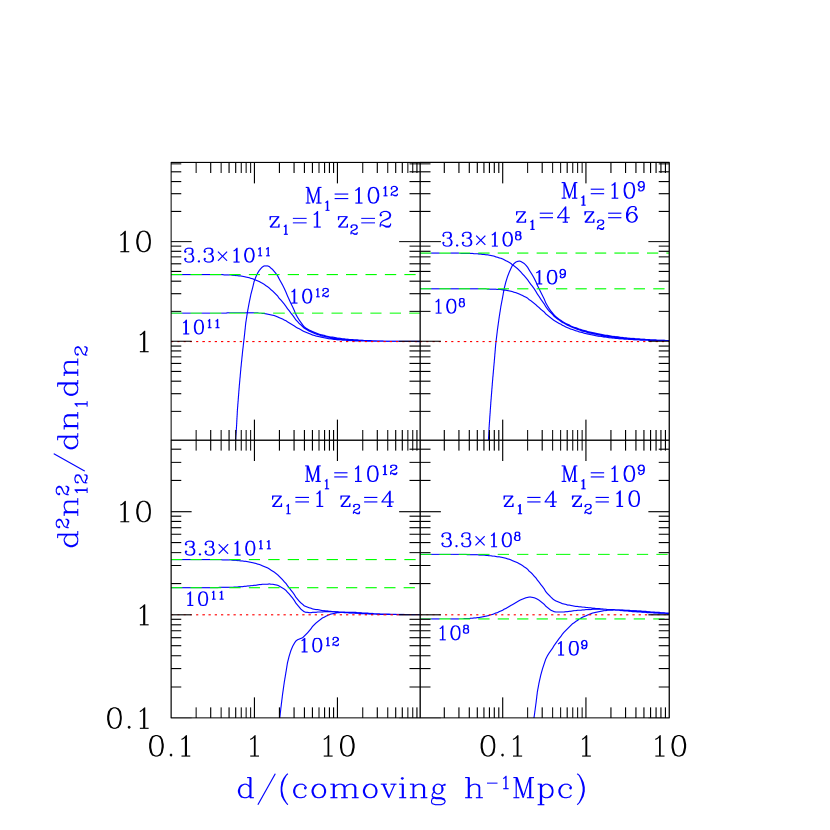
Figure 9: Normalized number density of halos as a function of $d$ for two objects forming at different redshifts. In the left panels we fix $M_{1}=10^{12}h^{-1}\,M_{\odot}$ and $z_{1}=1$, and consider $M_{2}$ values of $10^{11}$, $3.3\times 10^{11}$, and $10^{12}h^{-1}\,M_{\odot}$, at redshifts $z_{2}=2$ and $z_{2}=4.$ In the right panels, we consider a smaller, higher redshift object and fix $M_{1}=10^{9}h^{-1}\,M_{\odot}$ and $z_{4}=4$. In this case we take $M_{2}$ values of $10^{8}$, $3.3\times 10^{8}$, and $10^{9}h^{-1}\,M_{\odot}$, at redshifts $z_{2}=6$ and $z_{2}=10.$ Each solid line is labeled by its corresponding $M_{2}$ value, while the fully uncorrelated and fully-correlated cases are shown in all cases by the dotted and dashed lines respectively (except that for $M_{1}=M_{2}$, the fully-correlated limit is a normalized density of zero).

4.2 Bivariate Cumulative Mass Fraction and Nonlinear Bias

Returning to eq. (35), we can construct the fraction of trajectories that have been absorbed by both barriers. Writing $Q$ in terms of the $x$ integral and performing the appropriate $\delta_{1}$ and $\delta_{2}$ integrals this becomes

$$F(\nu_{1},\nu_{2},S_{1},S_{2},\xi)=\int_{-\infty}^{\nu_{\rm min}}dx\,\left[G(x,\xi)-G(2\nu_{\rm min}-x,\xi)\right]\,{\rm erf}\left(\frac{\nu_{1}-x}{\sqrt{2(S_{1}-\xi)}}\right){\rm erf}\left(\frac{\nu_{2}-x}{\sqrt{2(S_{2}-\xi)}}\right)\ .$$ (44)

This is the product of the mass fraction in halos of mass below $M_{1}(S_{1})$ at redshift $z_{1}(\nu_{1})$ and the mass fraction in halos of mass below $M_{2}(S_{2})$ at $z_{2}(\nu_{2})$, given that the distance between the halos is $d$. In other words, if we divide $F$ by the one-point value of the mass fraction in halos of mass $<M_{1}(S_{1})$ at $z_{1}(\nu_{1})$, we obtain the biased mass fraction in halos of mass $<M_{2}(S_{2})$ at $z_{2}(\nu_{2})$, where the biasing refers to an average only over points at a distance $d$ from the population of halos $<M_{1}(S_{1})$. In order to construct the correlation function of rare, massive halos, we instead need a closely related quantity; this is the “bivariate cumulative mass fraction,” that is the product of mass fractions in halos with masses above  $M_{1}$ and $M_{2}$, given by

$$F(\nu_{1},\nu_{2},<S_{1},<S_{2},\xi)=1+F(\nu_{1},\nu_{2},S_{1},S_{2},\xi)-{\rm erf}\left(\frac{\nu_{1}}{\sqrt{2S_{1}}}\right)-{\rm erf}\left(\frac{\nu_{2}}{\sqrt{2S_{2}}}\right)\ .$$ (45)

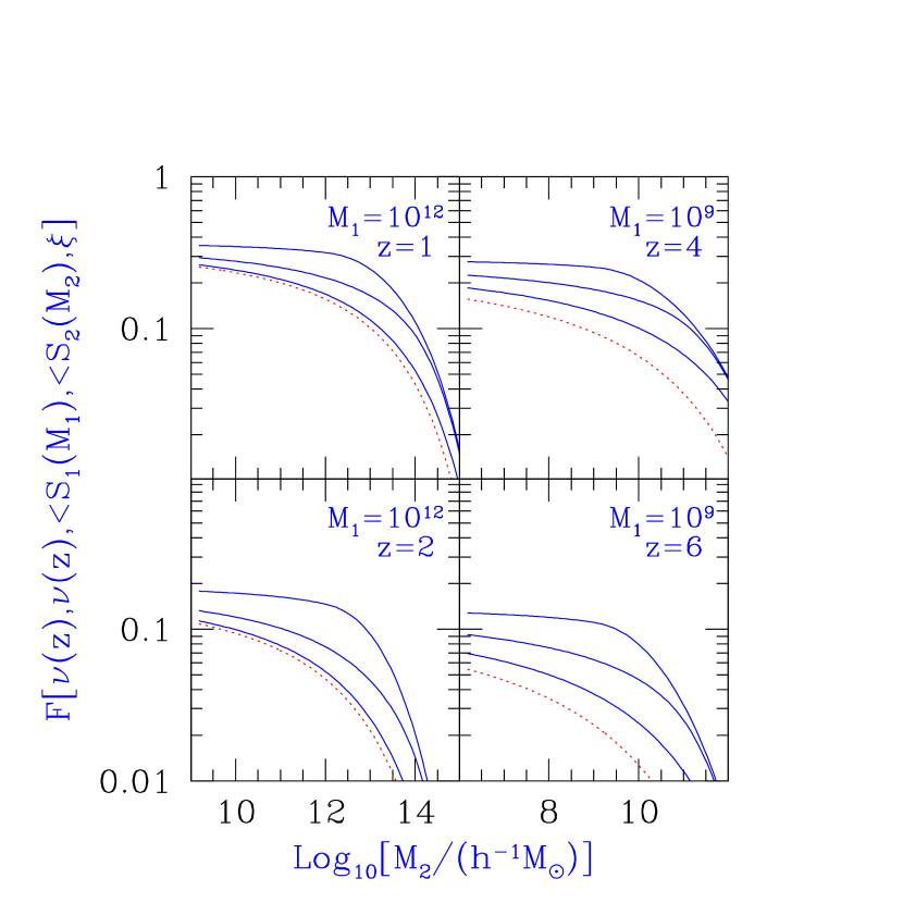
Figure 10: Bivariate cumulative mass fraction as a function of $M_{2}$, for various values of $d$, $M_{1}$, and $z$. In the left panels $M_{1}=10^{12}h^{-1}\,M_{\odot}$, and $z=$ 1 and 2. From top to bottom, the solid lines in these panels show $F$ values with the Lagrangian distances between the two points fixed at 1.0, 3.3, and 10 comoving $h^{-1}\,{\rm Mpc}$ respectively, and the uncorrelated case is shown for reference by the dotted lines. In the right panels, $M_{1}=10^{9}h^{-1}\,M_{\odot}$, and $z=$ 4 and 6. In these panels the solid lines show, from top to bottom, $F$ values with d = 0.1, 0.33, and 1.0 comoving $h^{-1}\,{\rm Mpc}$, while the dotted lines again correspond to the uncorrelated case.

In Figure 10 we plot $F(\nu_{1},\nu_{2},<S_{1},<S_{2},\xi)$, setting $S_{1}=\sigma^{2}(M_{1})$, $S_{2}=\sigma^{2}(M_{2})$, and $\xi=\xi_{r_{max}}(d)$, and fixing $\nu_{1}=\nu_{2}=\delta_{c}(z)$ at various redshifts. In the left panels of this figure we again set $M_{1}=10^{12}h^{-1}\,M_{\odot}$, $z=1$ and $2$, and $d=1$, 3.3, and 10 comoving $h^{-1}\,{\rm Mpc}$. At the smallest distances, the two points are almost completely correlated, and $F$ approaches its one-point value of ${\rm erfc}[\nu(z)/\sqrt{2\sigma^{2}(M_{\rm max})}]$ as given by eq. (12), where $M_{\rm max}$ is the greater of the two masses. This is because the plotted quantity expresses the joint probability of a halo of mass $>M_{1}$ at point $A$ and a halo $>M_{2}$ at point $B$. When the two points are very close together, both points are contained within the same halo, which therefore must have a mass greater than $M_{\rm max}$. Thus if, e.g., $d=1h^{-1}\,{\rm Mpc}$ and $M_{2}\leq M_{1}$, $F$ is roughly constant at a value corresponding to $M_{1}$, while $F$ quickly approaches ${\rm erfc}[\nu(z)/\sqrt{2\sigma^{2}(M_{2})}]$ when $d=1$ and $M_{2}>M_{1}$. Note also that at $d=3.3h^{-1}\,{\rm Mpc}$ the points are somewhat uncorrelated at small values of $M_{2}$, but at larger value of $M_{2}$ the overlap between the points becomes much larger, and thus they become almost completely correlated, moving towards the $d=1h^{-1}\,{\rm Mpc}$ case at the highest $M_{2}$ values. Finally, at $d=10h^{-1}\,{\rm Mpc}$, the points are almost uncorrelated and $F$ closely approximates the product of two independent one-point probabilities, as given by the dotted lines. At this large distance, correlations are only somewhat significant at the highest $M_{2}$ values, moving $F$ slightly away from the dotted lines.

In the right panels, we again consider $M_{1}=10^{9}h^{-1}\,M_{\odot}$, $z=4$ and $z=6$, and $d$ = 0.1, 0.33, and 1.0 comoving $h^{-1}\,{\rm Mpc}$. The main features are similar to those seen in the higher-mass cases, although the correlations between the two points are somewhat stronger, moving the $d$ = 1.0 and 0.33 curves away from the dotted, uncorrelated cases, and up towards the almost fully correlated $d$ = 0.1 line. Again this line is roughly constant at a value corresponding to $M_{1}$ for low values of $M_{2}$, and moves towards ${\rm erfc}[(\nu(z)/\sqrt{2\sigma^{2}(M_{2})}]$ at larger $M_{2}$ values, and again the correlations for the $d$ = 0.33 and 1.0 $h^{-1}\,{\rm Mpc}$ cases become more significant at large values of $M_{2}.$

Returning to eq. (45), we can also immediately obtain the biasing of rare halos; namely, the bias between halos of masses larger than $M(S)$ at a distance $d$ at a redshift $z(\nu)$, defined as the increase in the cumulative mass fraction at the second point given the presence of an object at the first point. This is simply given by the bivariate cumulative mass fraction divided by the cumulative mass fraction at two uncorrelated points,

$$\xi_{\nu,{\rm 2stp}}(d,S)+1=\left[{\rm erfc}\left({\frac{\nu}{\sqrt{2S}}}\right)\right]^{-2}F(\nu,\nu,<S,<S,\xi(d,S))\ .$$ (46)

This equation can be compared with the usual expression used for nonlinear bias (Kaiser, 1984), which we can rewrite in a form similar to eq. (44) as

$$\xi_{\nu,\rm K84}(d,S)+1=\left[{\rm erfc}\left({\frac{\nu}{\sqrt{2S}}}\right)\right]^{-2}\int_{-\infty}^{\infty}dx\,G(x,\xi)\,\left[{\rm erfc}\left(\frac{\nu-x}{\sqrt{2(S-\xi)}}\right)\right]^{2}.$$ (47)

This expression was derived by simply integrating over the distribution of probabilities at each of the two points, in a manner analogous to Press & Schechter’s original derivation of the one-point mass function. Thus, this expression suffers from the same peaks-within-peaks problem which forced Press & Schechter to multiply their expressions by an arbitrary factor of 2.

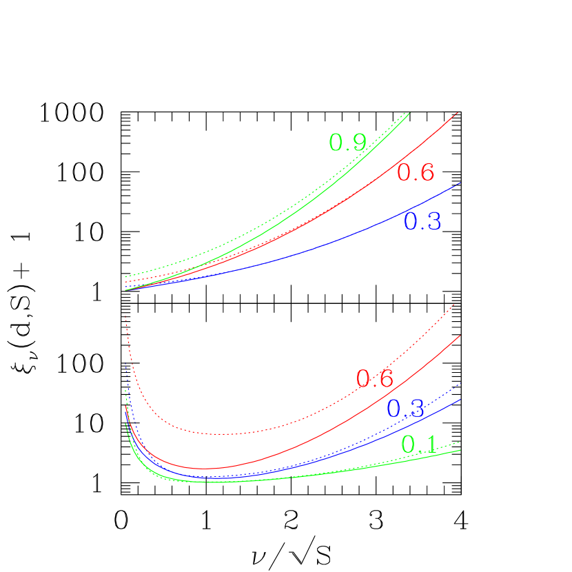
Figure 11: Nonlinear bias of rare peaks, as a function of $\nu/\sqrt{S}$. The cumulative bias is shown in the top panel; in each pair of curves the dotted line corresponds to the standard expressions derived in Kaiser (1984), while the (lower) solid line correspond to $\xi_{\nu,{\rm 2stp}}.$ Each pair of lines is labeled in terms of the scaled correlation between the two points, $\xi/S$, which is 0.9, 0.6, and 0.3, from top to bottom. The bias of halos at a given mass is shown in the bottom panel; in each pair of curves the dotted line shows the biased correlation function that is based on Mo & White (1996), while the solid line corresponds to $\hat{\xi}_{\nu,{\rm 2stp}}$. In this case $\xi/S$ values of 0.6, 0.3, and 0.1 are used, from top to bottom.

The bias between peaks as computed using the two-step approximation, eq. (46), and the one from the standard approach, eq. (47), are plotted in Figure 11 as a function of the height of the peak, in units of $\sqrt{S}$, for two perturbations of various correlation strengths $\xi/S$. This comparison helps clarify the range over which eq. (47) is most accurate, but it also makes clear that eq. (46) is a superior generalization which self-consistently accounts for all of the matter in the universe.

In the fully-correlated limit ($\xi\rightarrow S$), $\xi_{\nu,K84}+1$ is too high by a factor of 2, at all $\nu$. This is because in this case, the points are fully correlated so the joint fraction is $F_{1,2}=F_{1}$, where $F_{1}={\rm erfc}(\nu/\sqrt{2S})$ is the cumulative mass fraction of a single halo, and therefore the bias is given simply by $F_{1,2}/F_{1}^{2}=1/F_{1}$. While the two-step derivation leads to the correct bias in this limit, Kaiser’s derivation ignores the Press-Schechter factor of 2 caused by the problem of peaks within peaks, and thus $\xi_{\nu,K84}+1$ approaches $2/F_{1}.$ Note also that in the two-step case, for all values of $\xi/S$, at $\nu/\sigma\rightarrow 0$ the bias approaches 1. This is because every point is in a halo corresponding to some $\nu/\sigma>0$, and thus imposing $\nu/\sigma>0$ is no constraint at all and does not result in bias. In the Kaiser (1984) case, however, this mass conservation is not imposed and instead $\xi_{\nu,\rm K84}\rightarrow\xi/S$ as $\nu/\sigma\rightarrow 0$. Finally, at large values of $\nu$, when $\nu\gg\sigma/(1-\xi/S)$, the two expressions become equal. Note, however, that for sufficiently high values of $\xi/S$, $\xi_{\nu,{\rm K84}}$ suffers from the erroneous factor of 2 problem even in the case of extremely rare peaks.

Finally, we consider another definition of bias which is also commonly used. This definition is designed to yield more directly the (Lagrangian) correlation function among rare peaks at a given  mass $M$, rather than the bias among the cumulative halo population above some mass $M$. In our calculation, this correlation function is simply given by

$$\hat{\xi}_{\nu,{\rm 2stp}}(d,S)+1=\left[f(\nu,S)\right]^{-2}f(\nu,\nu,S,S,\xi(d,S))\ ,$$ (48)

where we refer to eqs. (10) and (41). In the absence of any previous derivation of this correlation function, even in the simple case corresponding to the assumptions of Kaiser (1984), previous efforts have resorted to defining the bias in other ways and hoping that these alternative definitions yield a value which is close to the desired correlation function. These methods include the “peak-background split”, which gives (Cole & Kaiser, 1989)

$$\hat{\xi}_{\nu,{\rm pk-bgd}}(d,S)=\frac{\xi}{S}\,\left(\frac{\nu^{2}/S-1}{\delta_{c}}\right)^{2}\ .$$ (49)

In testing these alternative definitions we assume that the ratio between the halo correlation function ($\hat{\xi}_{\nu,{\rm pk-bgd}}$ in this case) and the normalized mass correlation function ($\xi/S$) equals the square of the bias. Eq. (49) is derived only in the limit of rare halos and large $d$, so we consider its generalization (Mo & White, 1996),

$$\hat{\xi}_{\nu,{\rm MW96}}(d,S)=\frac{\xi}{S}\ \frac{\int_{-\infty}^{1}Q(\nu,\nu x,S)\left[\frac{f(\nu(1-x),S-S_{0})}{f(\nu,S)}-1\right]^{2}dx}{\int_{-\infty}^{1}Q(\nu,\nu x,S)\,\delta_{c}^{2}\,x^{2}\,dx}\ .$$ (50)

In this expression, $\delta_{c}=1.686$ (see §2) and $S_{0}$ is the $\sigma^{2}$ of the mass scale $M_{0}$, where a sphere (at the mean density) of comoving radius $d$ contains a mass $M_{0}$. Note that $\hat{\xi}_{\nu,{\rm MW96}}$ was calculated from eq. (43), using a definition of bias which considers the number density of halos of a given mass that form out of matter initially contained within larger overdense spheres. The comparison in Figure 11 (bottom panel) shows that $\hat{\xi}_{\nu,{\rm MW96}}$ successfully approximates $\hat{\xi}_{\nu,{\rm 2stp}}$ only when $\xi/S$ is small, and only over a limited range of values of $\nu/\sigma$. On the other hand, our result represents a direct analysis of the correlation function of halos, and at all parameter values it is fully consistent with the closely related bias $\xi_{\nu,{\rm 2stp}}$ of eq. (46).

The abundance of halos and their correlations are determined by the linear power spectrum, since the formation of a halo is a long-term process that is driven by the existence of initial overdensities. However, correlation functions involving parts of halos depend also on the non-linear, internal structure of the halos themselves. Examples include the autocorrelation function of galaxies, which depends on the variation with halo mass of the number of galaxies per halo, and the dark matter autocorrelation function, which depends on the internal density profiles of halos. Prescriptions for the internal structure of halos have been previously combined with the halo correlation function based on Mo & White (1996) to produce various autocorrelation functions (e.g., Seljak, 2000; Ma & Fry, 2000). These analyses can now be improved with our generalized, self-consistent results for halo correlations.

4.3 Bivariate Mixed-mass Function

The last quantity of interest is the bivariate mixed mass function, which is the mass function at one point times the correlated cumulative mass fraction at a second point,

$$\frac{dn_{1}F_{2}}{dM_{1}}=\frac{\bar{\rho}}{M_{1}}\left|\frac{dS_{1}}{dM_{1}}\right|{\cal F}(\nu_{1},\nu_{2},S_{1},S_{2},\xi)\ .$$ (51)

Using eqs. (37) and (38), this can be written as the sum of three terms:

$${\cal F} = 4\frac{\partial\xi}{\partial S_{1}}Q_{0}+\frac{\nu_{1}}{S_{1}}G(\nu_{1},S_{1})$$ (52)

$$- \int_{-\infty}^{\nu_{\rm min}}dx\,\left[G(x,\xi)-G(2\nu_{\rm min}-x,\xi)\right]\,\frac{\nu_{1}-x}{S_{1}-\xi}\,G(\nu_{1}-x,S_{1}-\xi)\,{\rm erf}\left(\frac{\nu_{2}-x}{\sqrt{2(S_{2}-\xi)}}\right),$$

where $Q_{0}$ is evaluated at $\delta_{1}=\nu_{1}$ and $\delta_{2}=\nu_{2}$.

In Figure 12 we plot this quantity, again normalizing by its limiting value at large distances,

$${\rm erfc}\left(\frac{\nu_{2}}{\sqrt{2S_{2}}}\right)\frac{\nu_{1}}{\sqrt{2\pi}S_{1}^{3/2}}\exp\left(-\frac{\nu_{1}^{2}}{2S_{1}}\right)\ ,$$ (53)

in order to emphasize its overall features. The plotted quantity equals the one-point mass function $f(\nu_{1},S_{1})$ of $M_{1}$ halos times the total mass fraction, at a distance $d$ away, in halos above mass $M_{2}$. In this plot we restrict our attention to halos that are able to cool in the neighborhood of the halo of mass $M_{1}$; for illustration we assume that molecular hydrogen formation is inefficient, and that star formation occurs only in galaxies in which atomic cooling is efficient. This in turn requires a halo virial temperature of at least $10^{4}$ K, which sets a minimum value of $M_{2}$ at each redshift.

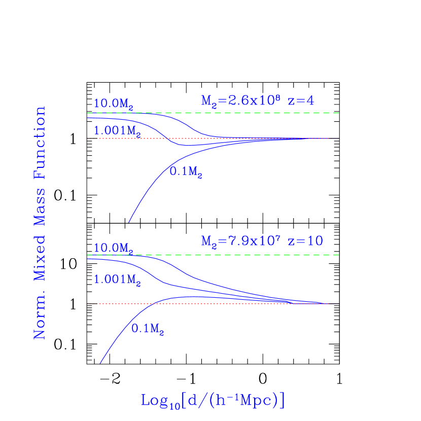
Figure 12: Bivariate Mixed-mass function. Upper panel:  each sold line shows ${\cal F}$ normalized by its uncorrelated value, as a function of $d$, for various values of $M_{1}$. The lines are labeled by their $M_{1}$ values and in all cases $z_{1}=z_{2}=4$, and $M_{2}$ is the cooling mass at this redshift, $2.6\times 10^{8}M_{\odot}$. For reference, the fully uncorrelated line is given by the dotted line and the fully correlated case in which $M_{1}>M_{2}$ is shown by the dashed line; if $M_{1}<M_{2}$ then the fully correlated case is zero. Lower panel:  Normalized ${\cal F}$ for a higher redshift case in which $z_{1}=z_{2}=10$, and $M_{2}$ is the (smaller) cooling mass at this redshift, $7.9\times 10^{7}M_{\odot}$, which corresponds to slightly rarer objects. The lines follow the same conventions as in the upper panel.

The figure shows that if $M_{1}$ is much smaller than $M_{2}$, then at small distances, the mass fraction above the cooling limit is zero, as no objects larger than $M_{1}$ form at this point. At intermediate values of the distance, however, the presence of a small object is able to either lower or raise the cooled mass fraction depending on how common or rare the objects are.

If $M_{2}$ is a generalized progenitor of $M_{1}$, however, so that $M_{1}>M_{2}$ and $z_{2}\geq z_{1}$, then we can compare ${\cal F}$ with the mixed mass function for two fully correlated points,

$${\rm erfc}\left[\frac{\nu_{2}-\nu_{1}}{\sqrt{2(S_{2}-S_{1})}}\right]\frac{\nu_{1}}{\sqrt{2\pi}S_{1}^{3/2}}\exp\left(-\frac{\nu_{1}^{2}}{2S_{1}}\right)\ ,$$ (54)

which corresponds to the dashed lines in the figure. In the case in which the two objects form at the same redshift, this is simply the mass function at a single point, as at short distances the presence of an object of a size larger than the cooling mass indicates that all the gas at this point has cooled. In general, the presence of a halo with $M_{1}>M_{2}$ can produce either a positive or negative overall bias in the amount of gas that cools within nearby halos, depending on $d$ and on $M_{1}$.

5 Conclusions

In this work, we have developed a simple but powerful extension of the Press & Schechter (1974) model that goes beyond Bond et al. (1991) and can be used to study inhomogeneous structure formation and correlation functions among halos. Although the linear excursion-set model represents the backbone of our modern analytical understanding of structure formation, it has previously only been able to predict the average number density of collapsed objects and has not supplied any information as to their relative positions. While many authors have derived approximate expressions for spatial correlations either analytically or from numerical simulations, each of these was grafted externally onto the underling formalism, leaving inhomogeneous structure formation on slippery theoretical ground.

Although a strict excursion set description of inhomogeneous structure formation can be constructed only by solving the diffusion equation numerically, we have shown in this work that such solutions can be matched to within $2\%$ accuracy using a simple approximation. By considering the trajectories of the overdensities at two points to be at first fully correlated and later fully uncorrelated as a function of decreasing filter scale, and by carefully choosing the cutoff value between these two regimes, we have developed an analytical formalism appropriate for studying problems in which a simple one-point approach is insufficient.

With this two-step approximation we are able to derive an approximation to the joint probability distribution for the overdensities of two points with arbitrary mass scales and collapse redshifts, separated by any comoving Lagrangian distance. This distribution leads directly to an analytical expression for the bivariate mass function of halos, given by eqs. (41) and (42), and for the bivariate cumulative mass fraction, given by eqs. (44) and (45). These expressions generalize a number of previous results, and also yield self-consistent expressions for the nonlinear biasing and correlation function of halos, given by eqs. (46) and (48). Our results also incorporate halo exclusion, i.e., the fact that if point $A$ belongs to a given halo, all nearby points $B$ are likely to belong to the same halo (see, e.g., Figure 7). We have also shown that the two-step approximation yields the right value in every limit where it must match a result derived from the one-point approach. We have provided Gemini  (see Appendix B), a publicly-available code that makes it easy to apply our formalism in specific cases.

Our results form an analytical framework that can be used in conjunction with numerical simulations to study inhomogeneous structure formation in a manner similar to the approach commonly adopted to study average quantities; analytical techniques are used to outline the overall physical picture and quantify model uncertainties, and numerical techniques are used to refine these results through a limited series of detailed tests. Likewise, these comparisons must take into account many of the issues that arise in a spatially averaged context, such as the best choice of collapse density $\delta_{c}$ (e.g., Kitayama & Suto, 1996; Sheth, Mo, & Tormen, 2001; Jenkins et al., 2001), possible corrections to the overall functional form of the mass function (e.g., Jenkins et al., 2001; Lee & Shandarin, 1998), and the relationship between the Eulerian coordinate system which is observed and the Lagrangian coordinates that are used in the excursion-set formalism (e.g., Mo & White, 1996; Catelan et al., 1998; Jing, 1999). While the study of such issues will sharpen the link between this formalism and more directly observable quantities, our method nevertheless already provides an important first step towards a better theoretical understanding of inhomogeneous structure formation. In this context the Lagrangian coordinate system intrinsic to an excursion-set description is a mixed blessing, for although it is more difficult to compare with simulations, it is usually much more important physically to have a measure of the total column depth of material separating two objects than their precise distance.

For many years the study of structure formation has centered on the formation of individual dark matter halos and their direct progenitors, yet many classes of problems that are now being studied can not be addressed in this context; and while it was once assumed that gravity alone controlled cosmic evolution, many more recent issues in structure formation are better described as an interplay between the IGM and the objects that form within it (e.g., Barkana & Loeb, 1999; Ciardi, Ferrara, & Abel, 2000; Scannapieco, Thacker & Davis, 2001). Each new generation of objects changes the state of the gas, and this state in turn affects the properties of the next generation to form.

¿From the dissociation of molecular hydrogen, to reionization and the resulting photoevaporation of halos, to the epoch of galactic winds, our universe has time after time undergone intense and inhomogeneous transformations. Although the intricacies of such processes will undoubtedly take years of observational and theoretical investigation to unravel, it is clear already that one’s answers will depend on one’s relative location.

Erratum

Immediately preceding the publication of this article we were alerted to the existence of a previous investigation into inhomogeneous structure formation from the point of view of excursion sets. In Porciani et al. (1998), the authors considered the simultaneous evolution of two points separated by a fixed initial comoving distance, but rather than approximate this evolution with a two-step procedure such as the one described in §3.3 of Scannapieco & Barkana (2002) they instead made use of the correlated two-point solution in the absence of barriers and imposed on this the same reflecting boundary conditions as in the fully uncorrelated case. In this way they were able to develop what amounts to an alternate approximation to our eq. (41) in the limited case of simultaneously collapsing halos.

While both approaches yield similar results at small values of $\xi/S$, the approximation proposed by Porciani et al. breaks down when the two points are highly correlated. In order to show this we consider the limit in which $\nu_{1}=\nu_{2}=\nu$, $S_{1}=S_{2}=S$ and $\xi\rightarrow S$, and restrict our attention to the physical range in which $\delta_{1},\delta_{2}\leq\nu$. In this case our two-step approximation simply reduces to the single absorbing barrier solution as given by eq. (28),

$$Q(\nu,\delta_{1},\delta_{2},S)=[G(\delta_{1},S)-G(2\nu-\delta_{1},S)]\,\delta_{D}(\delta_{1}-\delta_{2})\ ,$$ (55)

where $G(\delta,S)$ is a Gaussian of variance $S$ in the variable $\delta$ [as in eq. (4)], and $\delta_{D}$ is the one-dimensional Dirac delta function. In this notation, the correlated solution with uncorrelated boundary conditions as per eqs. (33) and (34) of Porciani et al. gives instead

$$Q(\nu,\delta_{1},\delta_{2},S)=[G(\delta_{1},S)+G(2\nu-\delta_{1},S)]\,\delta_{D}(\delta_{1}-\delta_{2}),$$ (56)

which amounts to an unphysical increase of probability density in the presence of absorbing barriers. This is because as $\xi\rightarrow S$, the double reflection as in the uncorrelated case becomes an increasingly poor approximation to the single reflection appropriate for correlated diffusion. Indeed, Figure 3 of Porciani et al. shows that their approximation fails to reproduce a numerical Monte Carlo solution when the two points are separated by a small distance; their approximation for the clustering properties of dark matter halos is accurate only for separations that are larger than the Lagrangian halo size by a factor of $\sim 3$–10, with the exact value depending on the power spectrum of density fluctuations and the halo mass.

Appendix A: Evaluation of the Bivariate Mass Function

In this Appendix we give various analytic expressions that are necessary for the explicit evaluation of eq. (41). Using eq. (31) to compute the derivatives, we find

$$\frac{\partial^{2}Q_{\pm}}{\partial\delta_{1}\partial\delta_{2}} = \frac{1}{4\pi(S_{1}S_{2}-\xi^{2})^{3/2}}\,\exp\left[-\,\frac{\delta_{1}^{2}S_{2}+\delta_{2}^{2}S_{1}-2\delta_{1}\delta_{2}\xi}{2(S_{1}S_{2}-\xi^{2})}\right]\ \times$$

$$\left\{\left[\frac{(\delta_{1}S_{2}-\delta_{2}\xi)(\delta_{2}S_{1}-\delta_{1}\xi)}{S_{1}S_{2}-\xi^{2}}+\xi\right]\,\left[{\rm erf}\left(\tilde{\nu}\sqrt{\frac{\tilde{S}}{2}}\right)\pm 1\right]\right.$$

$$-\left.\sqrt{\frac{2\tilde{S}}{\pi}}\exp\left(-\frac{\tilde{S}}{2}\tilde{\nu}^{2}\right)\left(\xi\frac{\nu_{\rm min}}{\tilde{S}}-\frac{\delta_{2}S_{1}}{S_{1}-\xi}-\frac{\delta_{1}S_{2}}{S_{2}-\xi}\right)\right\}\ ,$$

and

$$\frac{\partial^{2}Q_{\pm}}{\partial\delta_{2}^{2}} = \frac{1}{4\pi(S_{1}S_{2}-\xi^{2})^{3/2}}\,\exp\left[-\,\frac{\delta_{1}^{2}S_{2}+\delta_{2}^{2}S_{1}-2\delta_{1}\delta_{2}\xi}{2(S_{1}S_{2}-\xi^{2})}\right]\ \times$$

$$\left\{\left[\frac{(\delta_{2}S_{1}-\delta_{1}\xi)^{2}}{S_{1}S_{2}-\xi^{2}}-S_{1}\right]\,\left[{\rm erf}\left(\tilde{\nu}\sqrt{\frac{\tilde{S}}{2}}\right)\pm 1\right]\right.$$

$$-\sqrt{\frac{2\tilde{S}}{\pi}}\left.\exp\left(-\frac{\tilde{S}}{2}\tilde{\nu}^{2}\right)\left[\xi\frac{S_{1}-\xi}{S_{2}-\xi}\frac{\nu_{\rm min}}{\tilde{S}}+\frac{\delta_{1}\xi}{S_{2}-\xi}+\delta_{2}\frac{\xi^{2}+S_{1}(\xi-2S_{2})}{(S_{2}-\xi)^{2}}\right]\right\},$$

while to compute $\partial^{2}Q_{\pm}/\partial\delta_{1}^{2}$ we simply switch the 1 and 2 indices in all terms of the previous equation. Finally, we also require

$$\frac{\partial Q_{\pm}}{\partial\xi} = \frac{Q_{\pm}}{S_{1}S_{2}-\xi^{2}}\left[\delta_{1}\delta_{2}+\xi\left(1+\frac{2\delta_{1}\delta_{2}\xi-\delta_{1}^{2}S_{2}-\delta_{2}^{2}S_{1}}{S_{1}S_{2}-\xi^{2}}\right)\right]\ +$$ (59)

$$\frac{1}{4\pi\sqrt{S_{1}S_{2}-\xi^{2}}}\,\exp\left[-\,\frac{\delta_{1}^{2}S_{2}+\delta_{2}^{2}S_{1}-2\delta_{1}\delta_{2}\xi}{2(S_{1}S_{2}-\xi^{2})}\right]\ \times$$

$$\exp\left(-\frac{\tilde{S}}{2}\tilde{\nu}^{2}\right)\sqrt{\frac{\tilde{S}}{2\pi}}\left(2\frac{\partial\tilde{\nu}}{\partial\xi}+\frac{\tilde{\nu}}{\tilde{S}}\frac{\partial\tilde{S}}{\partial\xi}\right),$$

where

$$\frac{\partial\tilde{S}}{\partial\xi}=\frac{S_{1}S_{2}(S_{2}-2\xi)(S_{1}-2\xi)-\xi^{4}}{(S_{1}S_{2}-\xi^{2})^{2}}\ ,$$ (60)

and

$$\frac{\partial\tilde{\nu}}{\partial\xi}=-\frac{\nu_{\rm min}}{\tilde{S}^{2}}\frac{\partial\tilde{S}}{\partial\xi}-\frac{\delta_{1}}{(S_{1}-\xi)^{2}}-\frac{\delta_{2}}{(S_{2}-\xi)^{2}}\ ,$$ (61)

although in our standard cases this term is not needed as $\xi_{k}$ and $\xi_{r_{max}}$ are only functions of the smaller of any two given values $S_{1}$ and $S_{2}$ [see eq. (41)].

Appendix B: Gemini,  A Toolkit for Analytical Models of Inhomogeneous Structure Formation

In order to facilitate applications of the analytical model of inhomogeneous structure formation discussed in this paper, we have made public a program Gemini  that is intended to be a toolkit that can be used to quickly evaluate the most important quantities derived in this work. The program is divided into two main sections; the first, xiroutines,  contains routines that compute preliminary quantities including the mass correlation function, in an arbitrary cosmology, and the second, gemini,  uses these quantities to calculate the bivariate functions described in this work.

The routines that calculate $\xi(r,d),$ $\frac{d\xi}{d\sigma^{2}}(r,d),$ and $\sigma^{2}(r)$ need only be run once for any given cosmology, as xiroutines  constructs a table of such values indexed as functions of $\ln(r)$ and $\ln(d-r)$ with arbitrary resolution. Subsequent calls to xiroutines  then interpolate between these values using a cubic spline technique.

The routines contained in gemini,  on the other hand, are more fragmented, with the user determining which subroutines need to be included into the main program in order to calculate the quantities relevant to the problem at hand. In this case no tabulation is used and the bivariate mass function, $f$, is computed analytically. The cumulative mass fraction and mixed mass function, on the other hand, require a single numerical integration. These are carried out as a function of the following four variables,

$$s\equiv\frac{S_{1}-\xi}{\xi}\,,\,t\equiv\frac{\nu_{1}}{\sqrt{2(S_{1}-\xi)}}\,,\,u\equiv\frac{\nu_{2}-\nu_{1}}{\nu_{1}}\,,\,v\equiv\sqrt{\frac{S_{1}-\xi}{S_{2}-\xi}}\,,\,$$ (62)

which are chosen to have simple values in common limits such as $S_{1}=S_{2}$ or $\nu_{1}=\nu_{2}.$ In terms of these quantities and in the case in which $\nu_{1}\leq\nu_{2}$

$$F(\nu_{1},\nu_{2},S_{1},S_{2},\xi)=\sqrt{\frac{s}{\pi}}\ J(s,t,u,v)\ ,$$ (63)

where

$$J(s,t,u,v)=\int_{0}^{\infty}dx\,\left[e^{-s(t-x)^{2}}-e^{-s(t+x)^{2}}\right]\,{\rm erf}(x)\,{\rm erf}[v(tu+x)]\ ,$$ (64)

while the case in which $\nu_{1}\leq\nu_{2}$, is calculated by simply switching the 1 and 2 indices in eq. (63).

Finally, the $x$ integral for the mixed-mass function ${\cal F}$ can be written as

$$\frac{-1}{2\pi\sqrt{\xi}(S_{1}-\xi)^{1/2}}\ \left[(\nu_{1}-\nu_{2})\sqrt{\frac{2}{S_{1}-\xi}}\,K(s,t,u,v,w)+2L(s,t,u,v,w)\right]\ ,$$ (65)

where

$$K(s,t,u,v,w)=\int_{w}^{\infty}dx\,\left[e^{-s(t+tu-x)^{2}}-e^{-s(t+tu-2w+x)^{2}}\right]\,{\rm erf}(xv)\,e^{-(x-tu)^{2}}\ ,$$ (66)

and

$$L(s,t,u,v,w)=\int_{w}^{\infty}dx\,\left[e^{-s(t+tu-x)^{2}}-e^{-s(t+tu-2w+x)^{2}}\right]\,x\,{\rm erf}(xv)\,e^{-(x-tu)^{2}}\ .$$ (67)

In this case the lower bound on the integration is defined as $w\equiv\max(0,tu).$

Gemini  is available at the web address http://www.arcetri.astro.it/^∼evan/Gemini/ which also contains more detailed documentation regarding its use.

References

- Balbi et al. (2000) Balbi, A. et al. 2000, ApJ, 545, L1
- Barkana & Loeb (1999) Barkana, R. & Loeb, A. 1999, ApJ, 523, 54
- Bond et al. (1991) Bond, J. R., Cole, S., Efstathiou, G., & Kaiser, N. 1991, ApJ, 379, 440
- Catelan et al. (1998) Catelan, P., Lucchin, F., Matarrese, S., & Porciani, C. 1998, MNRAS, 297, 692
- Ciardi, Ferrara, & Abel (2000) Ciardi, B., Ferrara, A., & Abel, T. 2000, ApJ, 533, 594
- Cole & Kaiser (1989) Cole, S., & Kaiser, N. 1989, MNRAS, 237, 1127
- Efstathiou (1992) Efstathiou, G. 1992, MNRAS, 256, 43
- Efstathiou et al. (1988) Efstathiou, G., Frenk, C. S., White, S. D. M., & Davis, M. 1988, MNRAS, 235, 715
- Eisenstein & Hu (1999) Eisenstein, D. & Hu, W. 1999, ApJ, 511, 5
- Gnedin & Ostriker (1997) Gnedin, N. Y., & Ostriker, J. P. 1997, ApJ, 486, 581
- Haiman, Abel & Rees (2000) Haiman, Z., Abel, T., & Rees, M. J. 2000, ApJ, 534, 11
- Haiman, Rees & Loeb (1996) Haiman, Z., Rees, M. J., & Loeb, A. 1996, ApJ, 467, 522
- Jenkins et al. (2001) Jenkins, A. et al. 2001, MNRAS, 321, 372
- Jing (1998) Jing, Y. P. 1998, ApJ, 503, L9
- Jing (1999) Jing, Y. P. 1999, ApJ, 515, L45
- Kaiser (1984) Kaiser, N. 1984, ApJ, 284, L9
- Katz, Quinn, & Gelb (1993) Katz, N., Quinn, T., & Gelb, J. M. 1993, MNRAS, 265, 689
- Kitayama & Suto (1996) Kitayama, T. & Suto, Y. 1996, ApJ, 469, 480
- Knox, Scoccimarro, & Dodelson (1998) Knox, L., Scoccimarro, R., & Dodelson, S. 1998, Phys. Rev. Lett., 2004
- Komatsu & Kitayama (1999) Komatsu, E. & Kitayama, T. 1999, ApJ, 526, L1
- Lacey & Cole (1993) Lacey, C., & Cole, S. 1993, MNRAS, 262, 627
- Lee & Shandarin (1998) Lee J. & Shandarin, S. F. 1998, ApJ 500, 14
- Lee & Shandarin (1999) Lee J. & Shandarin, S. F. 1999, ApJ, 517, L5
- Ma & Fry (2000) Ma, C. & Fry, J. N. 2000, ApJ, 543, 503
- Menci (2001) Menci, N 2001, accepted to MNRAS, astro-ph/0111228
- Miralda-Escudé & Rees (1998) Miralda-Escudé, J. & Rees, M. J. 1998, ApJ, 497, 21
- Mo, Jing, & White (1996) Mo, H. J., Jing, Y. P., & White, S. D. M. 1996, MNRAS, 282, 1096
- Mo & White (1996) Mo, H. J. & White, S. D. M. 1996, MNRAS, 282, 347
- Monaco (1995) Monaco, P. 1995, ApJ, 447, 23
- Monaco (1997a) Monaco, P. 1997a, MNRAS, 287, 753
- Monaco (1997b) Monaco, P. 1997b, MNRAS, 290, 493
- Netterfield et al. (2001) Netterfield, C. B. et al. 2001, ApJ, submitted, (astro-ph/0104460)
- Peebles (1980) Peebles, P. J. E. 1980, The Large-Scale Structure of the Universe (Princeton: Princeton University Press)
- Press et al. (1992) Press, W. H., Teukolsky, S. A., Vetterling, W. T., & Flannery, B. P. 1992, Numerical Recipies in C: The Art of Scientific Computing, Second Ed. (Cambridge: Cambridge University Press)
- Press & Schechter (1974) Press, W. H., & Schechter, P. 1974, ApJ, 187, 425
- Pryke et al. (2001) Pryke, C. et al. 2001, ApJ, submitted (astro-ph/0104490)
- Scannapieco, Silk, & Tan (2000) Scannapieco, E., Silk, J. & Tan, J. C. 2000, ApJ, 529, 1
- Scannapieco & Broadhurst (2001) Scannapieco, E., & Broadhurst, T. 2001, ApJ, 549, 28
- Scannapieco, Thacker & Davis (2001) Scannapieco, E., Thacker, R. J., & Davis, M. 2001, ApJ, 557, 605
- Seljak (2000) Seljak, U. 2000, MNRAS, 318, 203
- Sheth, Mo, & Tormen (2001) Sheth, R. K., Mo, H. J., & Tormen, G. 2001, MNRAS, 323, 1