Measuring CMB Polarization with ESA PLANCK SubMM-Wave Telescope

Abstract

We analyze the polarization properties of the tilted off-axis dual-reflector submillimeter-wave telescope on the ESA PLANCK Surveyor designed for measuring the temperature anisotropies and polarization characteristics of the cosmic microwave background.

1 Introduction

The dual-reflector submillimeter-wave telescope on the ESA PLANCK Surveyor is being designed for measuring the temperature anisotropies and polarization characteristics of the cosmic microwave background (CMB).

Our research is concerned with one of its focal plane instruments, Far-IR High Frequency Instrument (HFI) [1], which will cover six frequency bands centered at $100$, $143$,$217$, $353$, $545$ and $857GHz$ providing the sensitivity of $\Delta T/T\sim 10^{-6}$ and the angular resolution down to $5$ arcminutes. The HFI consists of an array of $36$ horn antenna structures (Fig. 1, a) feeding the bolometric detectors which will be cryogenically cooled to a temperature of $100mK$.

One objective of the research is the optimization of the HFI optical design and the computation of the HFI beam patterns. The challenge of the problem is that the telescope is electrically large ($D/\lambda=4300$ at $\lambda=350\mu m$) and consists of two essentially defocused ellipsoidal reflectors providing a very large field of view at the focal plane.

Another objective is the characterization of the polarization properties of the multi-beam telescope system. The CMB polarization is expected to be at a level of only 10% of the temperature anisotropy quadrupole, and the success of the measurements will depend crucially on the precise knowledge of the polarization properties of the telescope.

2 Formulation of the problem

While the performance of the antenna structures can be thoroughly tested in terrestrial conditions, the coupling of the HFI with the telescope is, basically, optimized through the computer simulations.

Among various simulation techniques, physical optics (PO) is the most adequate one for the given purpose. However, conventional implementations of the technique [2, 3] do not fit the size of the problem. Commercially available packages are also very limited in their capacity to rigorously answer this sort of questions. For example, even the best commercial software requires many hours of the full-scale physical optics computation of the main beam of the telescope at the relatively low frequency of $143GHz$, while all conventional physical optics codes collapse at the highest frequencies of $545-857GHz$.

To solve the problem, we developed a special PO code [1] that allowed us to overcome the limitations of a generic approach for large multi-reflector systems and perform typical simulations of the telescope in the order of minutes. Generally, it requires only $1$ minute for a polarized Gaussian beam at the frequency of $143GHz$ and about $30$ minutes for the beam of $30$ modes at $857GHz$ using a PC Pentium III ($500MHz$) under the Linux operating system.

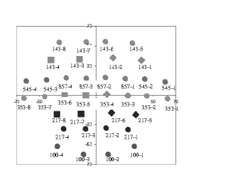
(a) (b)

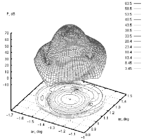
Figure 1: (a) Horn positions on the focal plane as seen from the telescope. (b) Total power of the telescope beam 143-1a computed for the clipped Gaussian feed model F3 with $a=3.9mm$, $w=2.8mm$, and $L=120mm$ ($f=143GHz$).

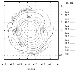
(a) (b)

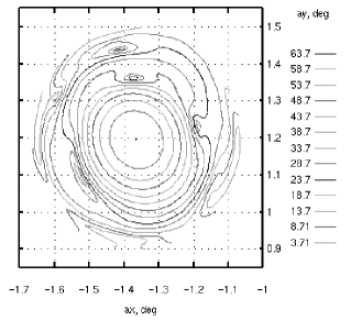
Figure 2: Power pattern of the telescope beam from the enhanced horn HFI-143-1a ($\psi_{a}=+45^{\circ}$, feed model F1) at the frequency (a) $121GHz$ and (b) $166GHz$.

We simulated the beams of twelve linearly polarized Gaussian horns operating in the transmitting mode at the nominal frequencies $143$, $217$, and $353GHz$. Each horn is designed for the simultaneous measurement of two orthogonal linear polarizations, ’a’ and ’b’, of the incoming radiation. The polarization is characterized by the tilt $\psi$ of the electric field at the beam axis in the sky with respect to the local vertical as defined below. The tilt is $\psi_{a}=+45^{\circ}$ and $\psi_{b}=-45^{\circ}$ for the horns 143-1, 143-2, 217-5, 217-6, 353-3, and 353-4 (see Fig. 1, a), while $\psi_{a}=0^{\circ}$ and $\psi_{b}=90^{\circ}$ for the other six polarized horns (the angle $\psi$ is measured clockwise from the upward vertical direction as seen from the telescope).

We compared three different models of the horn feed, F1, F2 and F3, when the source field is specified in different manner. The feed model F1 is represented by the far-field power and phase patterns of the actual corrugated horn in $0^{\circ}/45^{\circ}/90^{\circ}$ cuts which are used in a somewhat approximate manner for computing the incident complex-vector electromagnetic field on the secondary mirror. The feed F2 is specified by the ’clipped Gaussian’ model distribution of the horn aperture electric field which is accurately propagated to the secondary mirror and further through the system. Finally, the feed F3 is represented by the far-field patterns similar to the model F1 which, however, are computed precisely from the clipped Gaussian aperture field of the model F2 and then used in an approximate manner identical to the feed model F1.

The electric field at the aperture of the Gaussian horn in the feed models F2 and F3 is specified as

$$\vec{E}(r)=E_{0}\exp(-r^{2}/w_{a}^{2})\exp(-iqr^{2})\ \vec{e},\qquad 0\leq r\leq a\\$$ (1)

where $r$ is the radial coordinate, $w_{a}$ is the beam radius at the horn aperture, $a$ is the horn aperture radius, $q=\pi/\lambda L$, $L$ is the curvature radius of the wavefront at the aperture (approximately, $L$ is the horn slant length), and $\vec{e}=\vec{e}_{a,b}$ is the unit polarization vector ($\vec{E}(r)=0$ if $r>a$). The aperture model of this kind is quite accurate in representing the field of real Gaussian horns. In particular, both the power and phase patterns of such a horn computed at the frequency $100GHz$ coincide perfectly well with the experimental data available for the model Gaussian horn designed for this frequency. However, some discrepancies in the sidelobes at the level of about $-30dB$ appear for the horns specifically optimized for the higher angular resolution.

The comparison of the feed models F2 and F3 shows that the minor differences can only be observed in the polarization patterns at the periphery of the telescope beam while the power patterns of the main beam are identical for both models. The beams computed with the feed models F1 and F3 are also very similar when the parameters of the model F3 are properly adjusted. In this case, also, it is only the polarization at the periphery of the beam that differs slightly for different models while the power patterns are very similar even at the level below $-30dB$. Finally, the orientation of the polarization vector on the beam axis in the sky field is precisely the same for all the feed models, and the polarization pattern, in general, is rather independent of both the horn pattern and of the fine features of the propagation model used in the simulations. It proves that the far-field model F1 can safely be used for the simulation of the telescope beams from the real horns despite the approximations used in the model.

3 Polarization of the Gaussian beams

Fig. 1, b, shows the power pattern of the telescope beam H-143-1 as projected on the plane normal to the telescope line-of-sight at the $(0,0)$ point ($a_{x}$ and $a_{y}$ are the horizontal and vertical axes on the plane, respectively, measured in degrees). The beam axis is at the point $a_{x}=-1.3645^{\circ}$, $a_{y}=1.1975^{\circ}$ which is defined as the point of maximum power of the beam. The pattern is computed for the clipped Gaussian feed model F3 with adjusted parameters $a=3.9mm$, $w=2.8mm$, and $L=120mm$, simulating the enhanced horn operating at the frequency $f=143GHz$.

The beam is well shaped down to almost $-30dB$ below the maximum and can be approximated by a Gaussian function (at this level, the pattern does not depend on polarization) with the full beam width of $W_{min}=7.05$ arcmin and $W_{max}=7.50$ arcmin measured at $-3dB$. The polarization of the beam is generally elliptical except precisely at the beam axis where it remains linear. In order to achieve the required orientation of the polarization pattern in the sky, we should orient the polarization vector $\vec{e}$ properly on the horn aperture [1].

For immediate comparison of polarizations measured by different horns when scanning through the sky, we should use easily aligned directions in the sky as equivalent reference polarization axes for different beams. Such directions are the meridians in the spherical frame of the telescope, with the pole being the telescope spin axis tilted by $\eta=85^{\circ}$ with respect to the line-of-sight (the meridians define local verticals at various observation points while the parallels are local horizontals that constitute the orthogonal directions).

Now, we should define the reference axis for the polarization vector $\vec{e}$ of a tilted horn. We define the reference axis as the direction of $\vec{e}$ in the horn aperture plane that is projected on the vertical axis of the focal plane. The orientation of $\vec{e}$ is specified by the angle $\phi$ in the horn aperture plane measured from this reference in a clockwise direction when looking from the horn to the secondary mirror.

Using these definitions, we have found that the beam of the H-143-1 horn is polarized at its axis at the required angles of (a) $\psi_{a}=+45^{\circ}$ and (b) $\psi_{b}=-45^{\circ}$ if the horn polarization vector $\vec{e}$ is specified by the angle $\phi_{a}=+42.99^{\circ}$ and $\phi_{b}=-47.01^{\circ}$, respectively.

When the polarization vector $\vec{e}$ is properly oriented, the cross-polarized component of the far field measured along the respective orthogonal direction in the sky is minimized. In such a case, the power pattern of the cross-polarized component is, basically, determined by the power pattern of the semi-minor axis of the polarization ellipse at each observation point of the beam. This pattern is very much the same for any orientation of the polarization vector and can be approximated as follows

$$P_{cr}=P_{cr0}\ [(\theta/\theta_{0})\ \sin(\varphi-\varphi_{0})]^{p}\ \exp[(\theta/\theta_{0})^{q}]$$ (2)

where $P_{cr0},\ dB$, is the maximum power of the minor axis component achieved at the points specified by the polar angle $\theta_{0}$ and the azimuthal angles $\varphi_{0}\pm 90^{\circ}$ measured from the center of the pattern which is located at the beam axis (the values of the parameters in this approximation depend on the position of the horn considered but the magnitude of $P_{cr0}$ is, typically, more than $30dB$ below the maximum value of the total power of the beam).

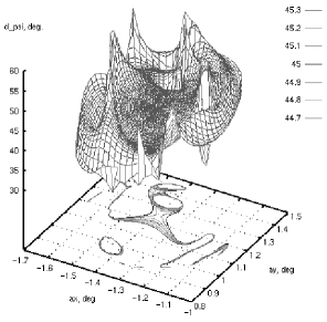
(a) (b)

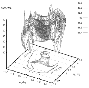
Figure 3: Deviation of the major axis of polarization ellipse from local vertical in the beam from the enhanced horn HFI-143-1a ($\psi_{a}=+45^{\circ}$, feed model F1) at the frequency (a) $121GHz$ and (b) $166GHz$.

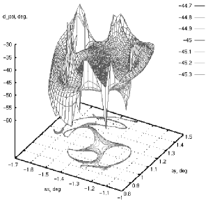
(a) (b)

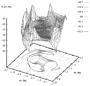
Figure 4: Deviation of the major axis of polarization ellipse from local vertical in the beam from the enhanced horn HFI-143-1b ($\psi_{b}=-45^{\circ}$, feed model F1) at the frequency (a) $121GHz$ and (b) $166GHz$

Since the actual frequency bands of the horns are rather wide ($121-166$, $182-252$, and $295-411GHz$), the far-field patterns of real horns differ essentially at the lower and upper frequencies of each band. It results in somewhat different power and polarization patterns of the telescope beam as shown in Figures 2 - 4. Nevertheless, despite these differences, the polarization angles at the beam axis are the same irrelevant of the horn patterns and of the operating frequency.

The values of the aperture polarization angle $\phi$ computed for all the HFI horns as well as the direction cosines (the Cartesian components of the unit vector) of the aperture electric field with respect to the coordinate frame $M1$ of the primary mirror are summarized in the Table 1.

Table 1: Orientation of the Polarization Vector $\vec{e}$ of the Aperture Electric Field

HFI horn	Aperture Angle		Unit Vector of the Aperture Electric Field
	$\phi$ [degrees]		$e_{X_{M1}}$		$e_{Y_{M1}}$		$e_{Z_{M1}}$
143-1-a	42.	99	0.	629015	0.	679549	0.	377562
143-1-b	-47.	01	0.	521115	-0.	728982	0.	443874
143-2-a	44.	17	0.	597142	0.	696388	0.	398076
143-2-b	-45.	83	0.	552563	-0.	716862	0.	425186
143-3-a	0.	82	0.	813844	0.	014303	0.	580907
143-3-b	-89.	18	0.	031357	-0.	999321	-0.	019324
143-4-a	2.	10	0.	812137	0.	036506	0.	582323
143-4-b	-87.	90	0.	080095	-0.	995568	-0.	049291
217-5-a	42.	99	0.	661010	0.	680077	0.	317114
217-5-b	-47.	01	0.	567397	-0.	729548	0.	381863
217-6-a	44.	11	0.	634880	0.	695677	0.	336097
217-6-b	-45.	89	0.	593249	-0.	717633	0.	364772
217-7-a	0.	89	0.	869188	0.	015525	0.	494238
217-7-b	-89.	11	0.	029397	-0.	999362	-0.	020308
217-8-a	2.	01	0.	867847	0.	034982	0.	495598
217-8-b	-87.	99	0.	066276	-0.	996754	-0.	045699
353-3-a	43.	70	0.	634926	0.	690048	0.	347422
353-3-b	-46.	30	0.	571370	-0.	722094	0.	390020
353-4-a	44.	70	0.	610581	0.	703339	0.	364012
353-4-b	-45.	30	0.	594981	-0.	710743	0.	375289
353-5-a	0.	58	0.	853206	0.	010120	0.	521476
353-5-b	-89.	42	0.	020092	-0.	999707	-0.	013472
353-6-a	1.	51	0.	852069	0.	026308	0.	522767
353-6-b	-88.	49	0.	052455	-0.	998000	-0.	035275

4 Conclusions

A fast physical optics code has been developed for the analysis of the dual-reflector submillimeter-wave telescope on the ESA PLANCK Surveyor. The code overcomes the limitations of a generic approach for large multi-reflector quasi-optical systems and can perform typical simulations of the telescope in the order of minutes.

Simulations of the telescope beams from the linearly polarized horns have shown that the far-field of the telescope is, generally, elliptically polarized except precisely at the beam axis where the linear polarization is preserved. The magnitude of the minor semi-axis of the polarization ellipse in the telescope beam remains at the level of $-30dB$ below the maximum total power of the beam even for the most tilted horns located at the edge of the HFI horn array.

When rotating the polarization vector of the horn field about the horn axis, the major axes of the polarization ellipses at the central part of the telescope beam rotate virtually by the same angle about the beam axis while the power patterns of both the co- and cross-polarized components of the far field remain basically unchanged.

Thus, the orthogonal polarization directions at the beam axis in the sky are transformed into the orthogonal directions in the focal plane of the telescope. Some deviations from this basic rule which occur mainly at the periphery of the beam are of minor importance since they virtually do not contribute to the measured total power of the polarized component.

5 Acknowledgments

The author is grateful to Bruno Maffei for the power and phase patterns of enhanced horns and to Yuying Longval for providing the updated positions and aiming angles of the HFI horns along with the map of the focal plane. The author would like to acknowledge the support of Enterprise Ireland.

References

- (1) Yurchenko, V., Murphy, J. A., and Lamarre, J. M., Int. J. Infrared and Millimeter Waves, 22, 173-184 (2001).
- (2) Diaz, L., and Milligan, T., Antenna Engineering Using Physical Optics: Practical CAD Techniques and Software, Artech House, London, 1996.
- (3) Scott, C., Modern Methods of Reflector Antenna Analysis and Design, Artech House, London, 1990.