Rotational velocities of A-type stars ^,

This work is the second part of the set of measurements of $v\sin i$ for A-type stars, begun by Royer et al. (2002). Spectra of 249 B8 to F2-type stars brighter than $V=7$ have been collected at Observatoire de Haute-Provence (OHP). Fourier transforms of several line profiles in the range 4200–4600 Å are used to derive $v\sin i$ from the frequency of the first zero. Statistical analysis of the sample indicates that measurement error mainly depends on $v\sin i$ and this relative error of the rotational velocity is found to be about 5 % on average.
The systematic shift with respect to standard values from Slettebak et al. (1975), previously found in the first paper, is here confirmed. Comparisons with data from the literature agree with our findings: $v\sin i$ values from Slettebak et al. are underestimated and the relation between both scales follows a linear law $v\sin i_{\mathrm{new}}=1.03\,v\sin i_{\mathrm{old}}+7.7$.
Finally, these data are combined with those from the previous paper (Royer et al. 2002), together with the catalogue of Abt & Morrell (1995). The resulting sample includes some 2150 stars with homogenized rotational velocities.

1 Introduction

This paper is a continuation of the rotational velocity study of A-type stars, initiated in Royer et al. (2002, hereafter Paper I). The main goals and motivations are described in the previous paper. The sample of A-type stars described and analyzed in this work is the counterpart of the one in Paper I, in the northern hemisphere.

In short, it is intended to produce a homogeneous sample of measurements of projected rotational velocities ($v\sin i$) for the spectral interval of A-type stars, and this without using any preset calibration.

This article is structured in a way identical to the precedent, except for an additional section (Sect. 5) where data from this paper, the previous one and the catalogue of Abt & Morrell (1995) are gathered, and the total sample is discussed in statistical terms.

2 Observational data

Spectra were obtained in the northern hemisphere with the AURÉLIE spectrograph (Gillet et al. 1994) associated with the 1.52 m telescope at Observatoire de Haute-Provence (OHP), in order to acquire complementary data to HIPPARCOS observations (Grenier & Burnage 1995).

The initial programme gathers early-type stars for which $v\sin i$ measurement is needed. More than 820 spectra have been collected for 249 early-type stars from January 1991 to May 1994. As shown in Fig. 1, B9 to A2-type stars represent the major part of the sample (70 %). Most of the stars are on the main sequence and only about one fourth are classified as more evolved than the luminosity class III-IV.

These northern stars are brighter than the magnitude $V=7$. Nevertheless, three stars are fainter than this limit and do not belong to the HIPPARCOS Catalogue (ESA 1997). Derivation of their magnitude from TYCHO observations turned out to be: HD 23643 $V=7.79$, HD 73576 $V=7.65$ and HD 73763 $V=7.80$. These additional stars are special targets known to be $\delta$ Scuti stars.

Figure 1: Distribution of the spectral type for the 249 programme stars.

AURÉLIE spectra were obtained in three different spectral ranges (Fig. 2):

• $\Lambda_{1}$: 4110–4310 Å. This domain was initially chosen to detect chemically peculiar stars by measuring equivalent widths of the lines Si ii 4128, Si ii 4131, Sr ii 4216, and Sc ii 4247.

• $\Lambda_{2}$: 4226–4432 Å or 4270–4475 Å. Centered around H$\gamma$, this spectral range allows the determination of the effective temperature.

• $\Lambda_{3}$: 4390–4600 Å, or 4400–4610 Å. This domain is dedicated to $v\sin i$ determination, although all the three ranges are used to measure the rotational velocity.

Two thirds of the sample have observations in each of the three ranges. The $\Lambda_{3}$ range is particularly aimed at $v\sin i$ measurement, and contains the largest number of lines selected for this purpose (twice as much as $\Lambda_{1}$ and $\Lambda_{2}$). Besides it is the only one which covers the magnesium doublet at 4481 Å. This line remains often alone for measurement in fast rotators. It is thus significant to note that among the 249 stars of the sample, three were observed only in the $\Lambda_{1}$ range, eight only in $\Lambda_{2}$ and eleven in both $\Lambda_{1}$ and $\Lambda_{2}$ only. Overall 22 stars have no observation in $\Lambda_{3}$. The reason is that these stars have already known $v\sin i$. Moreover they are effective temperature standard stars or reference stars for chemical abundances.

Some changes in the configuration of the instrument meant the central wavelengths of the $\Lambda_{2}$ and $\Lambda_{3}$ domains have been slightly modified during mission period.

The entrance of the slit is a 600 $\mu$m hole, i.e. 3″ on the sky, dedicated to the 1.52 m Coudé telescope. The dispersion of the collected spectra is 8.1  Å $\mathrm{mm}^{-1}$ and the resolving power is about 16 000.

The barrette detector is a double linear array TH 7832, made of 2048 photo-diodes. Reduction of the data has been processed using MIDAS procedures.

Flat field correction with a tungsten lamp and wavelength calibration with a Th-Ar lamp have been made with classical procedures. Nevertheless, a problem occurred when applying the flat-field correction with the tungsten calibration lamp. The division by the W lamp spectrum produced a spurious effect in the resulting spectrum at a given position in the pixels axis. This effect distorts the continuum, as it can be seen on the spectra of Vega (Fig. 2). This problem triggered the decision to change the instrumental configuration and central wavelengths of the spectral ranges.

Figure 2: Observed spectra of Vega are displayed for the different spectral ranges: top panel, range $\Lambda_{1}$; middle panel, range $\Lambda_{2}$; bottom panel, range $\Lambda_{3}$. Each domain covers nearly 200 Å.

• $\Lambda_{1}$: the first range extends from the red wing of H$\delta$ to the blue wing of H$\gamma$ which restricts the reliable normalization area. It contains seven of the selected lines.

• $\Lambda_{2}$: centered around H$\gamma$, this range only contains five selected lines.

• $\Lambda_{3}$: this range contains the largest number of selected lines, 16 in total, among which the doublet line Mg ii 4481.

The 23 selected lines (listed in Table 2) are indicated, and show up twice in the overlap areas.The instrumental feature coming from flat-fielding lamp is noticeable in the three spectra ($\sim 4280$ Å in $\Lambda_{1}$, $\sim 4390$ Å in $\Lambda_{2}$, $\sim 4560$ Å in $\Lambda_{3}$).

3 Measurement of the rotational velocity

The method adopted for $v\sin i$ determination is the computation of the first zero of Fourier transform (FT) of line profiles (Carroll 1933; Ramella et al. 1989). For further description of the method applied to our sample, see Paper I. The different observed spectral range induces some changes, which are detailed below.

3.1 Continuum tracing

The normalization of the spectra was performed using MIDAS: the continuum has been determined visually, passing through noise fluctuations. The procedure is much like the normalization carried out in Paper I, except for a different spectral window. For the ranges $\Lambda_{1}$ and $\Lambda_{2}$, the influence of the Balmer lines is important, and their wings act as non negligible contributions to the difference between true and pseudo-continuum, over the major part of the spectral domain, as shown in Paper I. On the other hand, the $\Lambda_{3}$ range is further from H$\gamma$. In order to quantify the alteration of continuum due to Balmer lines wings and blends of spectral lines, a grid of synthetic spectra of different effective temperatures (10 000, 9200, 8500 and 7500 K) and different rotational broadenings, computed from Kurucz’ model atmosphere (Kurucz 1993), is used to calculate the differences between the true continuum and the pseudo-continuum. The pseudo-continuum is represented as the highest points in the spectra. The differences are listed in Table 1, for different spectral 20 Å wide sub-ranges. This table is a continuation of the similar one in Paper I, considering the spectral range 4200–4500 Å.

Table 1: Differences between the true continuum and the highest points in different spectral bands for the set of synthetic spectra in the $\Lambda_{3}$ domain. Wavelength indicates the center of the 20 Å wide range.

$T_{\mathrm{eff}}$, $v\sin i$		central wavelength (Å)
(K, $\mathrm{km}\,\mathrm{s}^{-1}$)		4510	4530	4550	4570	4590
Data for wavelengths shorter than 4500 Å
are given in Table 1 of Paper I
10 000,	10	0.0005	0.0003	0.0002	0.0000	0.0000
10 000,	50	0.0008	0.0003	0.0003	0.0002	0.0003
10 000,	100	0.0011	0.0005	0.0016	0.0005	0.0013
9200,	10	0.0010	0.0006	0.0006	0.0006	0.0006
9200,	50	0.0017	0.0008	0.0010	0.0012	0.0012
9200,	100	0.0023	0.0012	0.0027	0.0012	0.0051
8500,	10	0.0017	0.0012	0.0010	0.0010	0.0010
8500,	50	0.0030	0.0020	0.0022	0.0025	0.0020
8500,	100	0.0042	0.0027	0.0062	0.0030	0.0093
7500,	10	0.0005	0.0005	0.0005	0.0005	0.0005
7500,	50	0.0032	0.0023	0.0036	0.0045	0.0032
7500,	100	0.0059	0.0050	0.0149	0.0059	0.0181

It is clear that the pseudo-continuum is much closer to the true continuum in $\Lambda_{3}$ than in both bluer ranges.

3.2 Set of lines

Put end to end, the spectra acquired with AURÉLIE cover a spectral range of almost 500 Å. It includes that observed with ECHELEC in Paper I. The choice of the lines for the determination of the $v\sin i$ in Paper I is thus still valid here. Moreover, in addition to this selection, were adopted redder lines in order to benefit from the larger spectral coverage.

The complete list of the 23 lines that are candidate for $v\sin i$ determination is given in Table 2.

Table 2: List of the 23 spectral lines used (when possible) for the $v\sin i$ measurement, and the corresponding spectral range(s) to which they belong.

range	wavelength	element	range
	4215.519	Sr ii
	4219.360	Fe i
	4226.728	Ca i
$\Lambda_{1}$	4227.426	Fe i
	4235.936	Fe i
	4242.364	Cr ii
	4261.913	Cr ii	$\Lambda_{2}$
	4404.750	Fe i
	4415.122	Fe i
	4466.551	Fe i
	4468.507	Ti ii
	4481${}^{.126}_{.325}$	Mg ii †
	4488.331	Ti ii
$\Lambda_{3}$	4489.183	Fe ii
	4491.405	Fe ii
	4501.273	Ti ii
	4508.288	Fe ii
	4515.339	Fe ii
	4520.224	Fe ii
	4522.634	Fe ii
	4563.761	Ti ii
	4571.968	Ti ii
	4576.340	Fe ii

† Wavelength of both components are indicated for the magnesium doublet line.

In order to quantify effects of blends in the selected lines for later spectral types, we use the skewness of synthetic line profiles, as in Paper I. The same grid of synthetic spectra computed using Kurucz’ model (Kurucz 1993), is used. Skewness is defined as $\gamma_{1}=m_{3}\,m_{2}^{-1.5}$, where $m_{k}$ is moment of $k$-th order equal to

$$\forall k,\;m_{k}={\displaystyle\sum_{i=1}^{L}\left[1-\mathscr{F}(\lambda_{i})\right]\left[\lambda_{i}-\lambda_{\mathrm{c}}\right]^{k}\over\displaystyle\sum_{i=1}^{L}1-\mathscr{F}(\lambda_{i})},$$ (1)

for an absorption line centered at wavelength $\lambda_{\mathrm{c}}$ and spreading from $\lambda_{1}$ to $\lambda_{L}$, where $\mathscr{F}(\lambda_{i})$ is the normalized flux corresponding to the wavelength $\lambda_{i}$. Ranges $[\lambda_{1},\lambda_{L}]$ are centered around theoretical wavelengths from Table 2 and the width of the window is taken to be 0.35, 0.90 and 1.80 Å for rotational broadening 10, 50 and 100 $\mathrm{km}\,\mathrm{s}^{-1}$ respectively (the width around the Mg ii doublet is larger: 1.40, 2.0 and 2.3 Å).

Table 3: Variation of the skewness $\gamma_{1}$ of the lines with $T_{\mathrm{eff}}$ and $v\sin i$ in the synthetic spectra.

	$v\sin i$	$T_{\mathrm{eff}}$ (K)
line	($\mathrm{km}\,\mathrm{s}^{-1}$)	10 000	9200	8500	7500
Data for wavelengths shorter than 4500 Å
are given in Table 3 of Paper I
Ti ii 4501	10	$-0.05$	$-0.06$	$-0.07$	$-0.12$
	50	$-0.02$	$-0.03$	$-0.04$	$-0.04$
	100	$-0.03$	$-0.04$	$-0.05$	$-0.07$
Fe ii 4508	10	$0.01$	$0.01$	$0.01$	$0.02$
	50	$-0.00$	$-0.00$	$-0.00$	$-0.00$
	100	$-0.01$	$-0.02$	$-0.03$	$-0.05$
Fe ii 4515	10	$0.00$	$-0.00$	$-0.01$	$-0.06$
	50	$0.02$	$0.02$	$0.01$	$-0.04$
	100	$0.01$	$0.01$	$0.02$	$0.03$
Fe ii 4520	10	$0.01$	$0.01$	$0.01$	$-0.01$
	50	$0.00$	$0.00$	$-0.00$	$-0.01$
	100	$-0.17$	$-0.19$	$-0.23$	$-0.30$
Fe ii 4523	10	$-0.06$	$-0.06$	$-0.06$	$-0.05$
	50	$-0.01$	$-0.01$	$-0.01$	$0.01$
	100	$-0.12$	$-0.09$	$-0.01$	$0.08$
Ti ii 4564	10	$0.04$	$0.04$	$0.05$	$0.06$
	50	$0.01$	$0.02$	$0.04$	$0.06$
	100	$0.03$	$0.04$	$0.08$	$0.16$
Ti ii 4572	10	$-0.00$	$-0.00$	$-0.01$	$-0.02$
	50	$0.01$	$0.00$	$-0.01$	$-0.09$
	100	$0.01$	$0.01$	$-0.00$	$-0.04$
Fe ii 4576	10	$0.01$	$0.01$	$0.02$	$0.05$
	50	$0.00$	$0.00$	$0.01$	$0.01$
	100	$0.01$	$0.02$	$0.04$	$0.07$

Table 3 lists the skewness of the lines for each element of the synthetic spectra grid and is a continuation of Table 3 from Paper I for the lines with wavelength longer than 4500 Å. These additional lines are rather isolated and free from blends. Major part of the computed $\gamma_{1}$ for the hotter spectrum (10 000 K) is far lower than the threshold 0.15 chosen in Paper I to identify occurrence of blends. The only case where a line must be discarded is the blend occurring with Fe ii 4520 and Fe ii 4523 for $v\sin i\gtrsim 100$ $\mathrm{km}\,\mathrm{s}^{-1}$. This non-blended behavior continues on the whole range of temperature, and the candidate lines remain reliable in most cases.

Figure 3: $v\sin i_{\mathrm{{Mg\textsc{ii}}}}$ derived from the 4481 Mg ii line versus $\langle v\sin i\rangle$ derived from other metallic lines for early A-type stars. The solid line stands for the one-to-one relation. The dashed line is the least-squares linear fit for $\langle v\sin i\rangle>30$ $\mathrm{km}\,\mathrm{s}^{-1}$.

Figure 4: Simulation of the doublet width behavior: $FWHM$ of the sum of two gaussian lines (separated with 0.2 Å) as a function of the $FWHM$ of the components.

The comparison between the rotational velocity derived from the weak lines and the one derived from the magnesium doublet was already approached in Paper I. It is here of an increased importance since the Mg ii line is not present in all spectra (i.e. $\Lambda_{1}$ and $\Lambda_{2}$ spectral ranges). Figure 3 shows this comparison between $\langle v\sin i\rangle$ and $v\sin i_{\mathrm{{Mg\textsc{ii}}}}$ using AURÉLIE data. The deviation from the one-to-one relation (solid line) in the low velocity part of the diagram is due to the intrinsic width of the doublet. This deviation is simulated by representing the Mg ii doublet as the sum of two identical gaussians separated by 0.2 Å. The full-width at half maximum ($FWHM$) of the simulated doublet line is plotted in Fig. 4 versus the $FWHM$ of its single-lined components. The relation clearly deviates from the one-to-one relation for single line $FWHM$ lower than 0.6 Å. Using the rule of thumb from Slettebak et al. (1975, hereafter SCBWP): $FWHM{\scriptstyle[\mathrm{\AA}]}\approx 0.025\,v\sin i{\scriptstyle[\mathrm{km}\,\mathrm{s}^{-1}]}$, this value corresponds to $v\sin i=24$ $\mathrm{km}\,\mathrm{s}^{-1}$. This limit coincides with what is observed in Fig. 3. For higher velocities ($\langle v\sin i\rangle>30$ $\mathrm{km}\,\mathrm{s}^{-1}$), $\langle v\sin i\rangle$ becomes larger than $v\sin i_{\mathrm{{Mg\textsc{ii}}}}$. A linear regression gives:

$$v\sin i_{\mathrm{{Mg\textsc{ii}}}}=0.88\,\langle v\sin i\rangle+2.2.$$ (2)

The effect is similar to the one found in Paper I, suggesting that blends in lines weaker than Mg ii produce an overestimation of the derived $v\sin i$ of about 10 %.

Figure 5: The average number of measured lines (running average over 30 points) is plotted as a function of the mean $\langle v\sin i\rangle$. Solid lines stands for the spectra collected with AURÉLIE ($\Lambda_{3}$ range) whereas dotted line represents ECHELEC spectra from Paper I.

The number of measurable lines among the 23 listed in Table 2 varies from one spectrum to another according to the wavelength window, the rotational broadening and the signal-to-noise ratio. The number of measured lines ranges from 1 to 17 lines. The $\Lambda_{3}$ range offers a large number of candidate lines. Fig. 5 shows the variation of this number with $v\sin i$ (solid line). Rotational broadening starts to make the number of lines decrease beyond about 70 $\mathrm{km}\,\mathrm{s}^{-1}$. Nevertheless additional lines in the spectral domain redder than 4500 Å makes the number of lines larger than in the domain collected with ECHELEC (Paper I; dotted line). Whereas with ECHELEC the number of lines decreases with $v\sin i$ from 30 $\mathrm{km}\,\mathrm{s}^{-1}$ to reach only one line (i.e. the Mg ii doublet) at 100 $\mathrm{km}\,\mathrm{s}^{-1}$, the number of lines with AURÉLIE is much sizeable: seven at 70 $\mathrm{km}\,\mathrm{s}^{-1}$, still four at 100 $\mathrm{km}\,\mathrm{s}^{-1}$ and more than two even beyond 150 $\mathrm{km}\,\mathrm{s}^{-1}$.

3.3 Precision

3.3.1 Effect of $v\sin i$

In Fig. 6, the differences between the individual $v\sin i$ values from each measured line in each spectrum and the associated mean value for the spectrum are plotted as a function of $\langle v\sin i\rangle$. In the same way the error associated with the $v\sin i$ has been estimated in Paper I, a robust estimate of the standard deviation is computed for each bin of 70 points. The resulting points (open grey circles in Fig. 6) are adjusted with a linear least squares fit (dot-dashed line). It gives:

$$\sigma_{v\sin i|v\sin i}=0.048{\scriptstyle\pm 0.010}\,\langle v\sin i\rangle+0.14{\scriptstyle\pm 0.19}.\\$$ (3)

This fit is carried out using GaussFit (Jefferys et al. 1998a, b), a general program for the solution of least squares and robust estimation problems. The resulting constant of the linear fit has an error bar of the same order than the value itself, and then the formal error is estimated to be 5 % of the $v\sin i$.

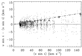
Figure 6: Differences between individual $v\sin i$ and mean over a spectrum $\langle v\sin i\rangle$. Variation of the standard deviation associated with the measure with the $\langle v\sin i\rangle$ is shown by the open circles. A linear least-square fit on these points (dot-dashed line) gives a slope of 0.05.

The slope is lower with AURÉLIE data than with ECHELEC spectra (Paper I): $4.8{\scriptstyle\pm 1.0}$ % against $5.9{\scriptstyle\pm 0.3}$ %. This trend can be explained by the average number of lines for the computation of the mean $v\sin i$. In the velocity range from 15 to 180 $\mathrm{km}\,\mathrm{s}^{-1}$, the number of measured lines (Fig. 5) is on average 2.4 times larger with AURÉLIE than with ECHELEC, which could lower the measured dispersion by a factor of $\sqrt{2.4}\approx 1.5$.

3.3.2 Effect of spectral range

As shown in Fig.1, the distribution of spectral types is mainly concentrated towards late-B and early-A stars, so that a variation of the precision as a function of the spectral type would not be very significant. On the other hand, as the observed spectral domain is not always the same, this could introduce an effect due to the different sets of selected lines, their quantity and their quality in terms of $v\sin i$ determination. For each of the three spectral domains, the residuals, normalized by $\sigma_{v\sin i|v\sin i}$ (Eq. 3), are centered around 0 with a dispersion of about 1 taking into account their error bars, as shown in Table 4. This suggests that no effect due to the measurement in one given spectral range is produced on the derived $v\sin i$.

Table 4: Mean of differences between individual $v\sin i$ and average $\langle v\sin i\rangle$ over a spectrum, normalized by the formal error due to $v\sin i$, are indicated for each spectral range as well as the standard deviations $\hat{\sigma}_{v\sin i|\Lambda}$ of these means.

Spectral range	$\left\langle{v\sin i-\langle v\sin i\rangle\over\sigma_{v\sin i|v\sin i}}\right\rangle$	$\hat{\sigma}_{v\sin i|\Lambda}$
$\Lambda_{1}$	$-0.04{\scriptstyle\pm 0.08}$	$1.00{\scriptstyle\pm 0.09}$
$\Lambda_{2}$	$-0.10{\scriptstyle\pm 0.12}$	$0.83{\scriptstyle\pm 0.13}$
$\Lambda_{3}$	$-0.03{\scriptstyle\pm 0.03}$	$0.92{\scriptstyle\pm 0.04}$

4 Rotational velocities data

4.1 Results

Table 5: (extract) Results of the $v\sin i$ measurements. Only the 15 first stars are listed below. The whole table is available electronically. Description of the columns is detailed in the text.

HD	HIP	Spect. type	$v\sin i$	$\sigma$	#	Remark
			($\mathrm{km}\,\mathrm{s}^{-1}$)
905	1086	F0IV	35	1	6
2421	2225	A2Vs	14	1	9
2628	2355	A7III	21	2	9
2924	2565	A2IV	31	2	16
3038	2707	B9III	184	–	1
4161	3572	A2IV	29	2	9
4222	3544	A2Vs	38	2	17
4321	3611	A2III	25:	4	14	SS
5066	4129	A2V	121	–	1
5550	4572	A0III	16	3	5
6960	5566	B9.5V	33	4	7
10293	7963	B8III	62	–	1
10982	8387	B9.5V	33	3	3
11529	9009	B8III	36	4	8
11636	8903	A5V…	73	2	11

In total, projected rotational velocities were derived for 249 B8 to F2-type stars, 86 of which have no rotational velocities in Abt & Morrell (1995).

The results of the $v\sin i$ determinations are presented in Table 5 which contains the following data: column (1) gives the HD number, column (2) gives the HIP number, column (3) displays the spectral type as given in the HIPPARCOS catalogue (ESA 1997), columns (4, 5, 6) give respectively the derived value of $v\sin i$, the associated standard deviation and the corresponding number of measured lines (uncertain $v\sin i$ are indicated by a colon), column (7) presents possible remarks about the spectra: SB2 (“SB”) and shell (“SH”) natures are indicated for stars showing such feature in these observed spectra, as well as the reason why $v\sin i$ is uncertain – “NO” for no selected lines, “SS” for variation from spectrum to spectrum and “LL” for variation from line to line (see Appendix A).

4.1.1 SB2 systems

Nine stars are seen as double-lined spectroscopic binary in the data sample. Depending on the $v\sin i$ of each component, their difference in Doppler shift and their flux ratio, determination of $v\sin i$ is impossible in some cases.

Figure 7: Part of the spectra are displayed for the six SB2 stars that have been observed only once: a) HD 35189, b) HD 40183, c) HD 42035, d) HD 181470, e) HD 203439, f) HD 203858. Three of them are well separated (b, d, f), allowing measurement of $v\sin i$ for both components. The three others (a, c, e) have low differential Doppler shift ($\leq 60$ $\mathrm{km}\,\mathrm{s}^{-1}$) which makes all the lines blended. No $v\sin i$ has been determined for these objects.

Figure 8: The three following SB2 stars have been observed twice, in $\Lambda_{1}$ (upper panels) and $\Lambda_{3}$ (lower panels): a) HD 79763 at HJD 2449025, b) HD 98353 at HJD 2448274, c) HD 119537 at HJD 2449025, d) HD 79763 at HJD 2449365, e) HD 98353 at HJD 2449413, f) HD 119537 at HJD 2449415. SB2 nature of these objects is not detected in $\Lambda_{1}$ spectral range, and the derived $v\sin i$ is a “combined” broadening. The triple system HD 98353 is observed close to conjunction, and lines remain blended. For HD 79763 (d) and HD 119537 (f), the difference in radial velocity is large enough to measure separately the rotational velocities.

Table 6 displays the results for the stars in our sample which exhibit an SB2 nature. Spectral lines are identified by comparing the SB2 spectrum with a single star spectrum. Projected rotational velocities are given for each component when measurable, as well as the difference in radial velocity $\Delta V_{\mathrm{r}}$ computed from a few lines in the spectrum.

Table 6: Results for stars seen as SB2. Rotational velocities are given for each component when measurable. $\Delta V_{\mathrm{r}}$ stands for the difference in radial velocity between the two components. Dash indicates a non possible measurement (either for $v\sin i$ or $\Delta V_{\mathrm{r}}$).

HD	HIP	Spect. type	$v\sin i$		$\Delta V_{\mathrm{r}}$	Fig.
			($\mathrm{km}\,\mathrm{s}^{-1}$)		($\mathrm{km}\,\mathrm{s}^{-1}$)
			A	B
35189	25216	A2IV	–		37	7a.
40183	28360	A2V	37	37	127	7b.
42035	29138	B9V	see text		12:	7c.
79763	45590	A1V	29		–	8a.
			34:	21:	67	8d.
98353	55266	A2V	44			8b.
			34		64:	8e.
119537	67004	A1V	20:		–	8c.
			17	18	98	8f.
181470	94932	A0III	15	20	229	7d.
203439	105432	A1V	–		56	7e.
203858	105660	A2V	14	15	106	7f.

• 110~Tau (HD 35189) is highly suspected to be a spectroscopic binary due to its spectra taken in the $\Lambda_{1}$ domain. As it can be seen in Fig. 7.a, core of the lines is double in most cases, corresponding to a difference in radial velocity of about 37 $\mathrm{km}\,\mathrm{s}^{-1}$. However, this case does not allow the measurement of the projected rotational velocity.

• $β$~Aur (HD 40183) is a well known early A-type eclipsing binary of Algol type. The derived $v\sin i$ corresponds well with the values of Nordström & Johansen (1994) (respectively 33 and 34 $\mathrm{km}\,\mathrm{s}^{-1}$) that indicate synchronous rotation. Knowing the time of minimum from Johansen & Sørensen (1997):

  $$\mathrm{HJD}_{\mathrm{min}}=2431076.7269+3.96004732\,E,$$

  where $E$ is an integer of phases, and the Julian date of observation (HJD 2449413.3301), the phase is equal to 0.4.

• HD~42035 has no indication of any binary status in the literature and it is flagged as a photometrically constant star from HIPPARCOS data. Nevertheless the observed line profiles in its spectrum tend to suggest that it is composite. The cross-correlation function (CCF) of the observed spectrum with a synthetic one ($T_{\mathrm{eff}}=10\,000$ K, $\log g=4.0$, $v\sin i=5$ $\mathrm{km}\,\mathrm{s}^{-1}$) has been computed. This CCF is not characteristic of a single star, and it is perfectly fitted by the sum of two gaussian components centered at 26 and 34 $\mathrm{km}\,\mathrm{s}^{-1}$ respectively and whose $FWHM$ are 30 and 120 $\mathrm{km}\,\mathrm{s}^{-1}$. This indicates that the system is composed of a low $v\sin i$ star and a faster rotator.

• HD~79763 is known as a SB2 system whose orbital period is $P=15.986$ d (Batten et al. 1989). Using the spectrum in $\Lambda_{3}$ range (Fig. 8.d), the difference in radial velocity is sufficient to estimate $v\sin i$ of both components.

• 55~UMa (HD 98353) is a triple system for which components are early A-type stars. Using tomographic separation, Liu et al. (1997) estimate the $v\sin i$ of each of them: $30\pm 4$ $\mathrm{km}\,\mathrm{s}^{-1}$, $45\pm 5$ $\mathrm{km}\,\mathrm{s}^{-1}$, $55\pm 5$ $\mathrm{km}\,\mathrm{s}^{-1}$. Knowing the orbital parameters: $P=2.5538380$ d and $T_{\mathrm{minRV}}=2449602.588$ (Horn et al. 1996) for the close pair, our spectra correspond to phases $\phi=0.99$ (Fig. 8.b, HJD 2448274.6233) and $\phi=0.02$ (Fig. 8.e, HJD 2449413.5500). This means that both observations were unfortunately made close to opposition, and the difference in radial velocity is not large enough to see separated lines. The measured $v\sin i$ corresponds to a blend.

• HD~119537 is indicated as SB in the Bright Star Catalogue (Hoffleit & Jaschek 1982) and was not detected as a double-lined system with the spectrum collected at ESO, within the context of the southern sample (Grenier et al. 1999; Royer et al. 2002). The rotational velocity derived in Paper I is $13\pm 1$ $\mathrm{km}\,\mathrm{s}^{-1}$, whereas it equals 23.9 $\mathrm{km}\,\mathrm{s}^{-1}$ in Ramella et al. (1989). The spectrum in the $\Lambda_{3}$ domain displays evidence of SB2 nature and Fig. 8.f shows perfectly the faint lines around Ti ii 4501, Fe ii 4508 and Ti ii 4515 which are usually well isolated in a single star with such a spectral type.

• HD~181470 is a close binary system first detected by speckle observations by Miura et al. (1993) and later confirmed by Hartkopf et al. (2000). The measured separation is $\rho=0\aas@@fstack{\prime\prime}13$ with a magnitude difference $\Delta m=1.6\pm 0.2$. In the observed spectrum, the difference in radial velocity is large: $229$ $\mathrm{km}\,\mathrm{s}^{-1}$.

• HD~203439 is known as a spectroscopic binary system in Batten et al. (1989).

• HD~203858 is a known spectroscopic binary. Abt & Morrell (1995) do not see the two components of the system and give a $v\sin i$ which is likely overestimated, 70 $\mathrm{km}\,\mathrm{s}^{-1}$, because of blend due to binarity. In this case, the components are well separated and each $v\sin i$ is measured.

4.2 Comparison with existing data

4.2.1 South versus North

Fourteen stars are common to both the southern sample from Paper I and the northern one studied here. Matching of both determinations allows us to ensure the homogeneity of the data or indicate variations intrinsic to the stars otherwise. Results for these objects are listed in Table 7.

Table 7: Comparison of the computed $v\sin i$ for the stars in common in the northern and southern samples (N $\equiv$ this work, S $\equiv$ Paper I). CFF is a flag indicating the shape of the cross-correlation function carried out by Grenier et al. (1999) using the ECHELEC spectra (0: symmetric and gaussian peak, 4: probable double, 5: suspected double, 6: probable multiple system).

HD	Sp. type	CCF	$v\sin i_{\mathrm{N}}$	$\sigma_{\mathrm{N}}$	$v\sin i_{\mathrm{S}}$	$\sigma_{\mathrm{S}}$
27962	A2IV	0	16	2	11	1
30321	A2V	4	132	4	124	–
33111	A3IIIvar	6	196	–	193	4
37788	F0IV	0	29	1	33	4
40446	A1Vs	–	27	5	27	5
65900	A1V	0	35	3	36	2
71155	A0V	4	161	12	137	2
72660	A1V	0	14	1	9	1
83373	A1V	0	28	–	30	2
97633	A2V	0	24	3	23	1
98664	B9.5Vs	–	57	1	61	5
109860	A1V	5	74	1	76	6
193432	B9IV	0	24	2	25	2
198001	A1V	0	130	–	102	–

Instrumental characteristics differ from ECHELEC to AURÉLIE data. First of all, the resolution is higher in the ECHELEC spectra, which induces a narrower instrumental profile and allows the determination of $v\sin i$ down to a lower limit. Taking the calibration relation from SCBWP as a rule of thumb ($FWHM{\scriptstyle[\mathrm{\AA}]}\approx 0.025\,v\sin i{\scriptstyle[\mathrm{km}\,\mathrm{s}^{-1}]}$), the low limit of $v\sin i$ is:

$$v\sin i_{\mathrm{lim}}={1\over 0.025}\,FWHM_{\mathrm{inst}}={1\over 0.025}\,{\lambda\over R},$$ (4)

where $R$ is the power of resolution, and $\lambda$ the considered wavelength. For ECHELEC spectra ($R\approx 28\,000$) this limit is 6.4 $\mathrm{km}\,\mathrm{s}^{-1}$ at 4500 Å, whereas for AURÉLIE data ($R\approx 16\,000$), it reaches 11.3 $\mathrm{km}\,\mathrm{s}^{-1}$. These limits correspond to the “rotational velocity” associated with the $FWHM$ of the instrumental profile. There is no doubt that in Fourier space, the position of the first zero of a line profile dominated by the instrumental profile is rather misleading and the effective lowest measurable $v\sin i$ may be larger. This effect explains the discrepancy found for slow rotators, i.e. HD 27962 and HD 72660 in Table 7. The $v\sin i$ determination using AURÉLIE spectra is 5 $\mathrm{km}\,\mathrm{s}^{-1}$ larger than using ECHELEC spectra. The two stars are slow rotators for which $v\sin i$ has already been derived using better resolution. HD 27962 is found to have $v\sin i=12$ and $11$ $\mathrm{km}\,\mathrm{s}^{-1}$ by Varenne & Monier (1999) and Hui-Bon-Hoa & Alecian (1998) respectively. HD 72660 has a much smaller $v\sin i$, lower than the limit due to the resolution of our spectra: 6.5 $\mathrm{km}\,\mathrm{s}^{-1}$ in Nielsen & Wahlgren (2000) and 6 $\mathrm{km}\,\mathrm{s}^{-1}$ in Varenne (1999).

Second of all, one other difference lies in the observed spectral domain. HD 198001 has no observation in the $\Lambda_{3}$ domain using AURÉLIE, so that $v\sin i_{\mathrm{N}}$ in Table 7 is not derived on the basis of the Mg ii line. The overestimation of $v\sin i_{\mathrm{N}}$ reflects the use of weak metallic lines instead the strong Mg ii line for determining rotational velocity.

Using the same ECHELEC data, Grenier et al. (1999) flagged the stars according to the shape of their cross-correlation function with synthetic templates. This gives a hint about binary status of the stars. Three stars in Table 7 are flagged as “probable binary or multiple systems” (CCF: 4 and 6).

When discarding low rotators, probable binaries and data of HD 198001 that induce biases in the comparison, the relation between the eight remaining points is fitted using GaussFit by:

$$v\sin i_{\mathrm{S}}=1.05{\scriptstyle\pm 0.04}\,v\sin i_{\mathrm{N}}-0.2{\scriptstyle\pm 1.5}.$$ (5)

Although common data are very scarce, they seem to be consistent. It suggests that both data sets can be merged as long as great care is taken for cases detailed above, i.e. extremely low rotators, high rotators with no $v\sin i$ from Mg ii line, spectroscopic binaries.

4.2.2 Standard stars

Figure 9: Comparison of $v\sin i$ data for the 163 common stars between this work and Abt & Morrell (1995). The solid line stands for the one-to-one relation.

Figure 10: Comparison between $v\sin i$ data from this work and from Slettebak et al. (1975). The solid line stands for the one-to-one relation. The 21 standard stars are plotted with error bar on both axes (see text). HD number of the stars that deviate most from the one-to-one relation are indicated and these stars are listed in Table 8 and detailed in Appendix B.

A significant part of the sample is included in the catalogue of Abt & Morrell (1995). The intersection includes 163 stars. The comparison of the $v\sin i$ (Fig. 9) shows that our determination is higher on average than the velocities derived by Abt & Morrell (AM). The linear relation given by GaussFit is:

$$v\sin i_{\mathrm{this\;work}}=1.18{\scriptstyle\pm 0.04}\,v\sin i_{\mathrm{AM}}+3.8{\scriptstyle\pm 0.8}.$$ (6)

Abt & Morrell use the standard stars of SCBWP to calibrate the relation $FWHM$–$v\sin i$. There are 21 stars in common between our sample and these standard stars. Figure 10 displays the $v\sin i$ derived in this paper versus the $v\sin i$ from SCBWP for these 21 common stars. The solid line represents the one-to-one relation. A clear trend is observed: $v\sin i$ from SCBWP are on average 20 % lower. A linear least squares fit carried out with GaussFit on these values makes the systematic effect explicit:

$$v\sin i_{\mathrm{this\;work}}=1.11{\scriptstyle\pm 0.07}\,v\sin i_{\mathrm{SCBWP}}+7.1{\scriptstyle\pm 1.7}.$$ (7)

The relation is computed taking into account the error bars of both sources. The error bars on the values of SCBWP are assigned according to the accuracy given in their paper (10 % for $v\sin i<200\,\mathrm{km}\,\mathrm{s}^{-1}$ and 15 % for $v\sin i\geq 200\,\mathrm{km}\,\mathrm{s}^{-1}$). Our error bars are derived from the formal error found in section 3.3 (Eq. 3).

Table 8: Highlight of the discrepancy between $v\sin i$ values from SCBWP and ours (standard deviation of our measurement is indicated; dash “–” stands for only one measurement). Comparison with data from the literature for the twelve stars that exhibit the largest differences. $v\sin i$ are classified in three subgroups according to the way they are derived: by-product of a spectrum synthesis, frequency analysis of the lines profiles or infered from a $FWHM$-$v\sin i$ relation independent from SCBWP’s one. Flags from HIPPARCOS catalogue are indicated: variability flag H52 (C: constant, D: duplicity-induced variability, M: possibly micro-variable, U: unsolved variable, –: no certain classification) and double annex flag H59 (O: orbital solution, G: acceleration terms, –: no entry in the Double and Multiple Systems Annex).

Name	HD	Sp. type	$v\sin i$ ($\mathrm{km}\,\mathrm{s}^{-1}$)						hipparcos
			scbwp	this work		literature			H52	H59
						spec. synth.	freq. analysis	$FWHM$
$\gamma$ Gem	47105	A0IV	$<10$	$15$	${\scriptstyle\pm 1}$	$11.2^{(1)}$	$10.2{\scriptstyle\pm 0.2}^{(2)}$, $19.0^{(3)}$		–	X
30 Mon	71155	A0V	$125$	$161$	${\scriptstyle\pm 12}$				C	–
$\beta$ UMa	95418	A1V	$35$	$47$	${\scriptstyle\pm 3}$	$44.8^{(1)}$, $39^{(4)}$	$44.3^{(3)}$		–	–
$\theta$ Leo	97633	A2V	$15$	$24$	${\scriptstyle\pm 3}$	$21^{(5)}$, $22.1^{(1)}$	$24^{(6)}$, $27.2^{(3)}$	$23^{(7)}$	–	–
$\gamma$ UMa	103287	A0V SB	$155$	$178$	${\scriptstyle\pm 9}$		$154{\scriptstyle\pm 4}^{(8)}$		M	–
$\alpha$ Dra	123299	A0III SB	$15$	$25$	${\scriptstyle\pm 2}$		$27^{(9)}$		M	O
$\sigma$ Boo	128167	F3Vwvar	$10$	$15$	${\scriptstyle\pm 1}$	$7.5{\scriptstyle\pm 1}^{(10)}$	$7.5^{(11)}$	$7.8^{(12)}$, $8.1^{(13)}$	–	–
$\alpha$ CrB	139006	A0V	$110$	$139$	${\scriptstyle\pm 10}$		$127{\scriptstyle\pm 4}^{(8)}$		U	O
$\tau$ Her	147394	B5IV	$30$	$46$	${\scriptstyle\pm 3}$		$32^{(6)}$		P	–
$\alpha$ Lyr	172167	A0Vvar	$<10$	$25$	${\scriptstyle\pm 2}$	$22.4^{(1)}$, $23.2^{(14)}$	$23.4{\scriptstyle\pm 0.4}^{(16)}$, $24^{(6)}$		U	–
						$21.8{\scriptstyle\pm 0.2}^{(15)}$	$29.9^{(3)}$
$\gamma$ Lyr	176437	B9III	$60$	$72$	${\scriptstyle\pm 2}$				M	–
$\epsilon$ Aqr	198001	A1V	$85$	$130$	–	$95^{(17)}$, $108.1^{(1)}$			–	–

(1) Hill (1995)	(6) Smith & Dworetsky (1993)	(11) Gray (1984)	(16) Gray (1980b)
(2) Scholz et al. (1997)	(7) Fekel (1998)	(12) Fekel (1997)	(17) Dunkin et al. (1997)
(3) Ramella et al. (1989)	(8) Gray (1980a)	(13) Benz & Mayor (1984)
(4) Holweger et al. (1999)	(9) Lehmann & Scholz (1993)	(14) Erspamer & North (2002)
(5) Lemke (1989)	(10) Soderblom (1982)	(15) Gulliver et al. (1994)

The standard stars for which a significant discrepancy occurs between our values and those derived by SCBWP – i.e. their error box does not intersect with the one-to-one relation – have their names indicated in Fig. 10. They are listed with data from the literature in Table 8 and further detailed in Appendix B.

5 Merging the samples

Homogeneity and size are two crucial characteristics of a sample, in a statistical sense. In order to gather a $v\sin i$ sample obeying these two criteria, $v\sin i$ derived in this paper and in Paper I can be merged with those of Abt & Morrell (1995). The different steps consist of first joining the new data, taking care of their overlap; then considering the intersection with Abt & Morrell, carefully scaling their data to the new ones; and finally gathering the complete homogenized sample.

5.1 Union of data sets from Paper I and this work (I $\cup$ II)

Despite little differences in the observed data and the way $v\sin i$ were derived for the two samples, they are consistent. The gathering contains 760 stars. Rotational velocity of common stars listed in Table 7 are computed as the mean of both values, weighted by the inverse of their variance. This weighting is carried on when both variances are available (i.e. $\sigma_{\mathrm{N}}^{2}$ and $\sigma_{\mathrm{S}}^{2}$), except for low rotators and HD 198001, for which $v\sin i_{\mathrm{S}}$ is taken as the retained value.

5.2 Intersection with Abt & Morrell and scaling

In order to adjust by the most proper way the scale from Abt & Morrell’s data to the one defined by this work and the Paper I, only non biased $v\sin i$ should be used. The common subsample has to be cleaned from spurious determinations that are induced by the presence of spectroscopic binaries, the limitation due to the resolution, uncertain velocities of high rotators with no measurement of the Mg ii doublet, etc. The intersection gathers 308 stars, and Fig. 11 displays the comparison.

We have chosen to adjust the scaling from Abt & Morrell’s data (AM) to ours (I $\cup$ II) using an iterative linear regression with sigma clipping. The least-squares linear fit is computed on the data, and the relative difference

$$\Delta=\left(v\sin i_{\mathrm{I}\cup\mathrm{II}}-(A\,v\sin i_{\mathrm{AM}}+B)\right)/v\sin i_{\mathrm{I}\cup\mathrm{II}},$$

where $A$ and $B$ are the coefficients of the regression line, is computed for each point. The standard deviation $\sigma_{\Delta}$ of all these differences is used to reject aberrant points, using the criterion :

$$|\Delta|>1.1\,\sigma_{\Delta}.$$

Then, the least-squares linear fit is computed on retained points and the sigma-clipping is repeated until no new points are rejected. One can see in previous section that points lying one sigma beyond their expected value are already significantly discrepant, this reinforces the choice of the threshold $1.1\,\sigma_{\Delta}$.

The 23 points rejected during the sigma-clipping iterations are indicated in Fig. 11 by open symbols. They are listed and detailed in Appendix C. Some of them are known as spectroscopic binaries. Moreover, using HIPPARCOS data, nine of the rejected stars are indicated as “duplicity induced variable”, micro-variable or double star. Half a dozen stars are low $v\sin i$ stars observed with AURÉLIE, and the resolution limitation can be the source of the discrepancy

Figure 11: Comparison of $v\sin i$ data for the 308 common stars between Abt & Morrell (1995) and the union of data from this work and from Paper I. Filled circles stand for stars from the “cleaned” intersection, that are used in the fit of Eq. 8, whereas open symbols represent stars discarded from the scaling fit (see text). The different open symbols indicate the possible reason why the corresponding stars are discarded: open square: known spectral binary system; open triangle: variability flag (H52) or binary flag (H59) in HIPPARCOS; open diamond: very low $v\sin i$ from AURÉLIE data; open circle: no reason. The solid line stands for the one-to-one relation. The dashed line is the fit carried on filled circles. All the discarded objects (open symbols) are listed and detailed in Appendix C.

The “cleaned” intersection, gathering 285 stars, is represented in Fig. 11 by filled circles. The solid line is the one-to-one relation and the dashed line represents the relation given by the iterative linear fit:

$$v\sin i_{\mathrm{I}\cup\mathrm{II}}=1.05\,v\sin i_{\mathrm{AM}}+7.5.$$ (8)

Rotational velocities from Abt & Morrell are scaled to the $v\sin i$ derived by Fourier transform (union of data sets from Paper I and this work), according to Eq. 8, in order to merge homogeneous data.

5.3 Final merging

Table 9 lists the 2151 stars in the total merged sample. It contains the following data: column (1) gives the HD number, column (2) gives the HIP number, column (3) displays the spectral type as given in the HIPPARCOS catalogue (ESA 1997), column (4) gives the derived value of $v\sin i$ (uncertain $v\sin i$, due to uncertain determination in either one of the source lists, are indicated by a colon).

Table 9: (extract) Results of the merging of $v\sin i$ samples. Only the 15 first stars are listed below. The whole table is available electronically. $\in$ stands for the membership and flags which sample stars belong to: 1, sample from Paper I; 2, sample from this work; 4, sample from Abt & Morrell (1995). This flag is set bitwise, so multiple membership is set by adding values together.

HD	HIP	Spect. type	$v\sin i$	$\in$
			($\mathrm{km}\,\mathrm{s}^{-1}$)
3	424	A1Vn	228	4
203	560	F2IV	170	4
256	602	A2IV/V	241	5
315	635	B8IIIsp…	81	4
319	636	A1V	59	5
431	760	A7IV	97	4
560	813	B9V	249	1
565	798	A6V	149	1
905	1086	F0IV	36	6
952	1123	A1V	75	4
1048	1193	A1p	28	4
1064	1191	B9V	128	1
1083	1215	A1Vn	233	4
1185	1302	A2V	128	4
1280	1366	A2V	102	4

The $v\sin i$ are attributed as the mean of available values weighted by the inverse of their variance. Trace of the membership to the different subsamples is kept and listed in column (5). The composition in terms of proportions of each subsample is represented as a pie chart in Fig. 12. The catalogue of Abt & Morrell contributes to the four fifths of the sample, and the remaining fifth is composed of new measurements derived by Fourier transforms.

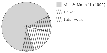
Figure 12: Pie chart of the subsample membership of the stars in the total $v\sin i$ sample. Multiple membership is represented by superimposed patterns.

The total sample is displayed in Fig. 13.a, as a density plot in equatorial coordinates. This distribution on the sky partly reflects the distribution in the solar neighborhood, and the density is slightly higher along the galactic plane (indicated by a dashed line). Note that the cell in equatorial coordinates with the highest density (around $\alpha=5$ h, $\delta=23\,\degr$) in Fig. 13.a corresponds to the position of the Hyades open cluster. The lower density in the southern hemisphere is discussed hereafter in terms of completeness of the sample.

5.4 Completeness

Except for a handful of stars, all belong to the HIPPARCOS catalogue. The latter is complete up to a limiting magnitude $V_{\mathrm{lim}}$ which depends on the galactic latitude $b$ (ESA 1997):

$$V_{\mathrm{lim}}=7.9+1.1\,\sin|b|.$$ (9)

This limit $V_{\mathrm{lim}}$ is faint enough for counts of A-type stars among the HIPPARCOS catalogue to allow the estimate of the completeness of the $v\sin i$ sample. This sample is north-south asymmetric because of the way it is gathered. Abt & Morrell observed A-type stars from Kitt Peak, and the range of declinations is limited from $\delta=-30\,\degr$ to $\delta=+70\,\degr$, and these limits can be seen in Fig. 13.a. Whereas the northern part of the sample benefits from the large number of stars in the catalogue from Abt & Morrell, the southern part mainly comes from Paper I. Thus the completeness is derived for each equatorial hemisphere. Figures 13.b and 13.c display the histograms in $V$ magnitude of the $v\sin i$ sample compared to the HIPPARCOS data, for $\delta>0\,\degr$ and $\delta<0\,\degr$ respectively. For both sources, only the spectral interval from B9 to F0-type stars is taken into account. Moreover data are censored, taking $V=8.0$ as the faintest magnitude.

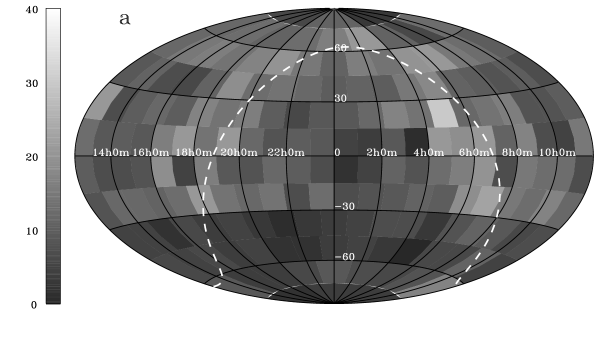
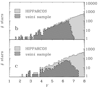
Figure 13: a) Density of the $v\sin i$ sample on the sky. Counts over 15°$\times$15° bins in equatorial coordinates are indicated by the grey scale. The dashed line stands for the galactic equator. b) and c) represent the counts in magnitude bins of the $v\sin i$ sample compared to the A-type stars in the HIPPARCOS catalogue for the northern and southern hemisphere respectively.

The completeness of the northern part is 80 % at $V=6.5$ mag. This reflects the completeness of the Bright Star Catalogue (Hoffleit & Jaschek 1982) from which stars from Abt & Morrell are issued. In the southern part, it can be seen that the distribution of magnitudes goes fainter, but the completeness is far lower and reaches 50 % at $V=6.5$ mag. These numbers apply to the whole spectral range from B9 to F0-type stars, and they differ when considering smaller spectral bins. For the A1-type bin for instance, the completeness reaches almost 90 % and 70 % for the northern and southern hemispheres respectively, at $V=6.5$ mag.

6 Summary and conclusions

The determination of projected rotational velocities is sullied with several effects which affect the measurement. The blend of spectral lines tends to produce an overestimated value of $v\sin i$, whereas the lowering of the measured continuum level due to high rotation tends to lower the derived $v\sin i$. The solution lies in a good choice of candidate lines to measure the rotational velocity. The use of the additional spectral range 4500–4600 Å, compared to the observed domain in Paper I, allows for the choice of reliable lines that can be measured even in case of high rotational broadening and reliable anchors of the continuum, for the considered range of spectral types. The $v\sin i$ is derived from the first zero of Fourier transform of line profiles chosen among 23 candidate lines according to the spectral type and the rotational blending. It gives resulting $v\sin i$ for 249 stars, with a precision of about 5 %.

The systematic shift with $v\sin i$ standard stars from SCBWP, already detected in Paper I, is confirmed in this work. SCBWP’s values are underestimated, smaller by a factor of 0.8 on average, according to common stars in the northern sample. When joining both intersections of northern and southern samples with standard stars from SCBWP, the relation between the two scales is about $v\sin i=1.03\,{v\sin i}_{\mathrm{SCBWP}}+7.7$, using these 52 stars in common. This is approximately our findings concerning the catalogue made by Abt & Morrell (1995). They derive their $v\sin i$ from the calibration built by SCBWP, and reproduce the systematic shift.

In the aim of gathering a large and homogeneous sample of projected rotational velocities for A-type stars, the new data, from the present paper and from Paper I, are merged with the catalogue of Abt & Morrell. First, the $v\sin i$ from the latter catalogue are statistically corrected from the above mentioned systematic shift. The final sample contains $v\sin i$ for 2151 B8- to F2-type stars.

The continuation of this work will consist in determining and analyzing the distributions of rotational velocities (equatorial and angular) for different sub-groups of spectral type, starting from the $v\sin i$.

Appendix A notes on stars with uncertain rotational velocity

A.1 Stars with no selected line

In a few cases, the selected lines are all discarded either from their Fourier profile or from their skewness (Table 3). For these stars, an uncertain value of $v\sin i$ is derived from the lines that should have been discarded. They are indicated by a colon and flagged as “NO” in Table 5. These objects are listed below. It is worth noticing that none of them have spectra collected in $\Lambda_{3}$ spectral range:

• HD~27459 and HD~27819 are early-F and late-A type stars from Hyades open cluster. Due to their rotational broadening and their late spectral type, no lines are retained in $\Lambda_{1}$. Their uncertain $v\sin i$ are respectively 78: and 41: $\mathrm{km}\,\mathrm{s}^{-1}$. Varenne & Monier (1999) measure their rotational velocity and find 78 and 47 $\mathrm{km}\,\mathrm{s}^{-1}$.

• HD~32537 is a early-F type star, whose $v\sin i$ derived from discarded line in $\Lambda_{1}$ is 27: $\mathrm{km}\,\mathrm{s}^{-1}$. The rotational velocity measured by Hui-Bon-Hoa (2000) is 21 $\mathrm{km}\,\mathrm{s}^{-1}$.

• HD~53929 is a late-B giant star, its spectra in $\Lambda_{1}$ exhibit very few lines. The $v\sin i$ is derived from Fe ii 4233 that is usually discarded because blended. For this spectral type, blend of the iron line is less pronounced, and the $v\sin i$ is 25: $\mathrm{km}\,\mathrm{s}^{-1}$. Dworetsky et al. (1998) find the same value.

• Following stars are high rotators whose only measurable line in $\Lambda_{1}$ is the blended line Fe ii 4233.

  • HD~59059, 260: $\mathrm{km}\,\mathrm{s}^{-1}$

  • HD~77104, 183: $\mathrm{km}\,\mathrm{s}^{-1}$

  • HD~111469, 197: $\mathrm{km}\,\mathrm{s}^{-1}$

  • HD~224404, 190: $\mathrm{km}\,\mathrm{s}^{-1}$

A.2 Stars with high external error

A few stars of the sample exhibit an external error higher than the estimation carried on in Sect. 3.3. It can be the signature of a multiple system. The following stars have variable $v\sin i$ from spectrum to spectrum and are labeled as “SS” in Table 5:

• HD~4321 has a mean $v\sin i=25\pm 4$ $\mathrm{km}\,\mathrm{s}^{-1}$, but for its different spectra, this value is respectively 38, $22\pm 3$ and $25\pm 1$ $\mathrm{km}\,\mathrm{s}^{-1}$.

• HD~40446 has a mean $v\sin i=27\pm 5$ $\mathrm{km}\,\mathrm{s}^{-1}$ (respectively 27, 32 and 22 $\mathrm{km}\,\mathrm{s}^{-1}$). The HIPPARCOS solution for this object is flagged “suspected non single”.

• HD~40626 has a mean $v\sin i=18\pm 3$ $\mathrm{km}\,\mathrm{s}^{-1}$  ($16\pm 1$ and $20\pm 1$ $\mathrm{km}\,\mathrm{s}^{-1}$). The $v\sin i$ found by Ramella et al. (1989) is 10.8 $\mathrm{km}\,\mathrm{s}^{-1}$.

• HD~103578 has a mean $v\sin i=16\pm 4$ $\mathrm{km}\,\mathrm{s}^{-1}$  ($14\pm 1$, $19\pm 1$ $\mathrm{km}\,\mathrm{s}^{-1}$). It is a SB2 system, and Hummel et al. (2001) who study its orbital motion, find $11.03\pm 0.14$ $\mathrm{km}\,\mathrm{s}^{-1}$ and $8.12\pm 0.27$ $\mathrm{km}\,\mathrm{s}^{-1}$ for the $v\sin i$ of each component.

Appendix B notes on $v\sin i$ standard stars with discrepant rotational velocity

The common stars, among SCBWP’s data and this sample, which exhibit the largest differences in $v\sin i$ between both studies, are listed in Table 8. They are detailed below.

• Alhena ($\gamma$ Gem, HD 47105) is a single-lined spectroscopic binary with a solar-type companion (Scholz et al. 1997). Hill (1995) carries out spectral synthesis on some A-type stars in the aim of deriving abundances and finds $v\sin i=11.2$ $\mathrm{km}\,\mathrm{s}^{-1}$ for $\gamma$ Gem. Scholz et al. measure the velocity using Fourier techniques on three spectral lines around 6 150 Å and derived $v\sin i=10.2\,\mathrm{km}\,\mathrm{s}^{-1}\,\pm 0.2\,\mathrm{km}\,\mathrm{s}^{-1}$. These two measurements are close to the value given by SCBWP: $<10$ $\mathrm{km}\,\mathrm{s}^{-1}$.

• 30~Mon (HD 71155) has no determination of $v\sin i$ in the literature, independent from Slettebak’s systems. It is nevertheless a common star between this work and Paper I, as described in Sect. 4.2.1. The “probable binarity” of 30 Mon, detected by Grenier et al. (1999) could explain the discrepancy in $v\sin i$. It is worth noticing that discrepancy is also observed with the $v\sin i$ determined in Paper I for this same object (Table 7).

• Merak ($\beta$ UMa, HD 95418) is known as a “Vega-type” star, supposed to be surrounded by protoplanetary material (Aumann 1985). Hill derives its $v\sin i$ as a sub-product of its abundance analysis. The value of 44.8 $\mathrm{km}\,\mathrm{s}^{-1}$ is significantly larger than the one found by SCBWP and is well in agreement with ours.

• $θ$~Leo (HD 97633) is studied by Fekel (1998), Lemke (1989) and Hill (1995), who give $v\sin i$ quite in agreement with our derived value, as already pointed out in Paper I. Smith & Dworetsky (1993) apply Fourier method to IUE spectra to derive $v\sin i$ for B and early A-type stars. Their finding for $\theta$ Leo is 24 $\mathrm{km}\,\mathrm{s}^{-1}$.

• Phecda ($\gamma$ UMa, HD 103287) is a spectroscopic binary. Gray (1980a) uses FT of the Mg ii line profile and derives $v\sin i=154\,\pm 4\,\mathrm{km}\,\mathrm{s}^{-1}$.

• Thuban ($\alpha$ Dra, HD 123299) is a well-known single-lined spectroscopic binary. Lehmann & Scholz (1993) use Bessel functions on the profile of Mg ii 4481 and derive a $v\sin i=27$ $\mathrm{km}\,\mathrm{s}^{-1}$ almost identical to the value found in this paper. Adelman et al. (1987) derive a lower velocity, but still larger than 15 $\mathrm{km}\,\mathrm{s}^{-1}$ given by SCBWP.

• $σ$~Boo (HD 128167) is a slowly rotating F-type star. Fitting the line profiles with synthetic ones, Soderblom (1982) derives $v\sin i=7.5$ $\mathrm{km}\,\mathrm{s}^{-1}$. Gray (1984), using Fourier method, finds an identical value. From the width of the CORAVEL cross-correlation function, Benz & Mayor (1984) derive $v\sin i=8.1\,\pm 0.8$ $\mathrm{km}\,\mathrm{s}^{-1}$ and from the width of the spectral lines, Fekel (1997) finds 7.8 $\mathrm{km}\,\mathrm{s}^{-1}$.

• Alphecca ($\alpha$ CrB, HD 139006) is an Algol-type eclipsing binary. The primary component is an A0V-type star and its projected rotational velocity is estimated at 110 $\mathrm{km}\,\mathrm{s}^{-1}$ by SCBWP. Gray (1980a) finds $v\sin i=127\,\mathrm{km}\,\mathrm{s}^{-1}\,\pm 4\,\mathrm{km}\,\mathrm{s}^{-1}$ from Fourier analysis.

• $τ$~Her (HD 147394) is a slowly pulsating B star whose period derived from HIPPARCOS data is $P=1.25$ d. Masuda & Hirata (2000) detect the line-profile variation by studying He i 4471 and Mg ii 4481. These variations could imply changes in the derived rotational velocity as both SCBWP’s and ours rely partly on Mg ii 4481. Smith & Dworetsky (1993) derive, using Fourier method, $v\sin i=32$ $\mathrm{km}\,\mathrm{s}^{-1}$.

• Vega ($\alpha$ Lyr, HD 172167) used to serve as a zero rotation standard, when limited spectral resolution prevented detection of low $v\sin i$. The rotational velocity given by SCBWP is $<10$ $\mathrm{km}\,\mathrm{s}^{-1}$. Gray (1980b) disagrees with this “distinctly too small” value and finds with Fourier techniques a larger value: 23.4 $\mathrm{km}\,\mathrm{s}^{-1}$ $\pm 0.4$ $\mathrm{km}\,\mathrm{s}^{-1}$. Vega is now suspected to be a rapid rotator nearly seen pole-on, and Hill (1995), Gulliver et al. (1994) and Erspamer & North (2002) using synthetic spectra, derive its $v\sin i$ and respectively give 22.4, 21.8 $\mathrm{km}\,\mathrm{s}^{-1}$ $\pm 0.2$ $\mathrm{km}\,\mathrm{s}^{-1}$, and 23.2 $\mathrm{km}\,\mathrm{s}^{-1}$.

• $γ$~Lyr (HD 176437) has no indication of $v\sin i$ determination or spectral peculiarity in the literature.

• $ϵ$~Aqr (HD 198001) has a $v\sin i=85$ $\mathrm{km}\,\mathrm{s}^{-1}$ according to SCBWP, smaller than the value in this work. As already mentioned in Sect. 4.2.1, this star has not been observed in $\Lambda_{3}$ spectral range, so that the derived $v\sin i$ is probably overestimated. Nevertheless, $\epsilon$ Aqr also belongs to the sample measured in Paper I and was already found discrepant, with a $v\sin i$ rather in agreement with those derived by Hill and Dunkin et al. (1997).

Appendix C notes on common stars with Abt & Morrell (1995) rejected by sigma-clipping

When merging the sample from Abt & Morrell (1995) with the new measurements using Fourier transforms, common data are compared in order to compute the scaling law between both samples. Aberrant points are discarded using a sigma-clipping algorithm. These stars are listed and discussed, and their $v\sin i$ are indicated in $\mathrm{km}\,\mathrm{s}^{-1}$ ($v\sin i_{\mathrm{I}\cup\mathrm{II}}/v\sin i_{\mathrm{AM}}$):

• HD~18778 (26 / 43) is a spectroscopic binary whose period is measured by Abt (1961): $P_{\mathrm{orb}}=11\aas@@fstack{d}665$. Its $v\sin i$ is found to be 20 $\mathrm{km}\,\mathrm{s}^{-1}$ by Dobrichev (1985).

• HD~27962 (11 / 15) is a binary star from HIPPARCOS data.

• HD~29573 (26 / 31) is detected as variable from HIPPARCOS observations, with unsolved solution.

• HD~32115 (12 / 15).

• HD~33204 (160 / 45) is an Am star in Hyades and is the primary component of the triple system ADS 3730. It is detected as a binary star by HIPPARCOS. Debernardi et al. (2000) compute the orbital parameters of this SB1 star, and derive its $v\sin i=24.0\pm 2.4$ $\mathrm{km}\,\mathrm{s}^{-1}$.

• HD~37594 (14 / 15)^⋆.

• HD~43760 (9 / 15) is suspected to be variable in radial velocity (Hui-Bon-Hoa 2000), and its $v\sin i$ is found to be 13 $\mathrm{km}\,\mathrm{s}^{-1}$.

• HD~50644 (12 / 13)^⋆ is indicated as micro-variable in the HIPPARCOS catalogue. Speckle observations (Hartkopf et al. 1997) allow the measurement of the separation of the system components $\rho=0\aas@@fstack{\prime\prime}159$.

• HD~71297 (11 / 13)^⋆ is a suspected binary from HIPPARCOS data.

• HD~72660 (9 / 10)^⋆ is a low rotator $v\sin i=6.5$ $\mathrm{km}\,\mathrm{s}^{-1}$ in Nielsen & Wahlgren (2000) and 6 $\mathrm{km}\,\mathrm{s}^{-1}$ in Varenne (1999).

• HD~111786 (45 / 135) is a periodic variable star in the HIPPARCOS catalogue. Its spectrum is composite (Faraggiana et al. 2001) and HD 111786 appears to be a multiple system.

• HD~115604 (15 / 15)^⋆.

• HD~132145 (15 / 30) has also been observed by Ramella et al. (1989) who find $v\sin i=16.6$ $\mathrm{km}\,\mathrm{s}^{-1}$.

• HD~158716 (15 / 35) has also been observed by Ramella et al. (1989) who find $v\sin i=19.6$ $\mathrm{km}\,\mathrm{s}^{-1}$.

• HD~159082 (21 / 30) has also been observed by Ramella et al. (1989) who find $v\sin i=19.6$ $\mathrm{km}\,\mathrm{s}^{-1}$. SB $P_{\mathrm{orb}}=6.79750$ (Stickland & Weatherby 1984)

• HD~159480 (28 / 40) is analyzed by Lemke (1989) who derives a $v\sin i$ from spectral synthesis: 27 $\mathrm{km}\,\mathrm{s}^{-1}$. HD 159480 has a negative result in speckle interferometry (McAlister et al. 1987).

• HD~159834 (18 / 28).

• HD~160839 (40 / 51).

• HD~175687 (10 / 10)^⋆.

• HD~187340 (15 / 33).

• HD~192640 (86 / 35) is an unsolved variable star in the HIPPARCOS catalogue.

• HD~203858 (14 / 70) is a spectroscopic binary. Miura et al. (1993), using speckle interferometry, estimate the separation between components $\rho<0\aas@@fstack{\prime\prime}039$.

• HD~208108 (28 / 35) has also been observed by Ramella et al. (1989) who find $v\sin i=29.0$ $\mathrm{km}\,\mathrm{s}^{-1}$.

^⋆: these stars show very coherent values between both samples, but these low $v\sin i$ are considered “discrepant” with respect to the scaling law (Eq. 8).

References

- Abt (1961) Abt, H. A. 1961, ApJS, 6, 37
- Abt & Morrell (1995) Abt, H. A. & Morrell, N. I. 1995, ApJS, 99, 135
- Adelman et al. (1987) Adelman, S. J., Bolcal, C., Kocer, D., & Inelmen, E. 1987, PASP, 99, 130
- Aumann (1985) Aumann, H. H. 1985, PASP, 97, 885
- Batten et al. (1989) Batten, A. H., Fletcher, J. M., & MacCarthy, D. G. 1989, 8th Catalogue of the orbital elements of spectroscopic binary systems (Victoria: Dominion Astrophysical Observatory)
- Benz & Mayor (1984) Benz, W. & Mayor, M. 1984, A&A, 138, 183
- Carroll (1933) Carroll, J. A. 1933, MNRAS, 93, 478
- Debernardi et al. (2000) Debernardi, Y., Mermilliod, J.-C., Carquillat, J.-M., & Ginestet, N. 2000, A&A, 354, 881
- Dobrichev (1985) Dobrichev, V. 1985, Astrofizicheskie Issledovaniya Sofia, 4, 40
- Dunkin et al. (1997) Dunkin, S. K., Barlow, M. J., & Ryan, S. G. 1997, MNRAS, 286, 604
- Dworetsky et al. (1998) Dworetsky, M. M., Jomaron, C. M., & Smith, C. A. 1998, A&A, 333, 665
- Erspamer & North (2002) Erspamer, D. & North, P. 2002, A&A, 383, 227
- ESA (1997) ESA. 1997, The Hipparcos and Tycho Catalogues, ESA-SP 1200
- Faraggiana et al. (2001) Faraggiana, R., Gerbaldi, M., Bonifacio, P., & François, P. 2001, A&A, 376, 586
- Fekel (1997) Fekel, F. C. 1997, PASP, 109, 514
- Fekel (1998) Fekel, F. C. 1998, in Precise stellar radial velocities, IAU Colloquium 170, ed. J. B. Hearnshaw & C. D. Scarfe, E64
- Gillet et al. (1994) Gillet, D., Burnage, R., Kohler, D., et al. 1994, A&AS, 108, 181
- Gray (1980a) Gray, D. F. 1980a, PASP, 92, 771
- Gray (1980b) —. 1980b, PASP, 92, 154
- Gray (1984) —. 1984, ApJ, 281, 719
- Grenier & Burnage (1995) Grenier, S. & Burnage, R. 1995, in De l’utilisation des données Hipparcos, ed. M. Frœschlé & F. Mignard, GDR 051, 177
- Grenier et al. (1999) Grenier, S., Burnage, R., Faraggiana, R., et al. 1999, A&AS, 135, 503
- Gulliver et al. (1994) Gulliver, A. F., Hill, G., & Adelman, S. J. 1994, ApJ Lett., 429, L81
- Hartkopf et al. (2000) Hartkopf, W. I., Mason, B. D., McAlister, H. A., et al. 2000, AJ, 119, 3084
- Hartkopf et al. (1997) Hartkopf, W. I., McAlister, H. A., Mason, B. D., et al. 1997, AJ, 114, 1639
- Hill (1995) Hill, G. M. 1995, A&A, 294, 536
- Hoffleit & Jaschek (1982) Hoffleit, D. & Jaschek, C. 1982, The Bright Star Catalogue, 4th edn. (New Haven, Conn.: Yale University Observatory)
- Holweger et al. (1999) Holweger, H., Hempel, M., & Kamp, I. 1999, A&A, 350, 603
- Horn et al. (1996) Horn, J., Kubát, J., Harmanec, P., et al. 1996, A&A, 309, 521
- Hui-Bon-Hoa (2000) Hui-Bon-Hoa, A. 2000, A&AS, 144, 203
- Hui-Bon-Hoa & Alecian (1998) Hui-Bon-Hoa, A. & Alecian, G. 1998, A&A, 332, 224
- Hummel et al. (2001) Hummel, C. A., Carquillat, J.-M., Ginestet, N., et al. 2001, AJ, 121, 1623
- Jefferys et al. (1998a) Jefferys, W. H., Fitzpatrick, M. J., & McArthur, B. E. 1998a, Celest. Mech., 41, 39
- Jefferys et al. (1998b) Jefferys, W. H., Fitzpatrick, M. J., McArthur, B. E., & McCartney, J. E. 1998b, GaussFit: A System for least squares and robust estimation, User’s Manual, Dept. of Astronomy and McDonald Observatory, Austin, Texas
- Johansen & Sørensen (1997) Johansen, K. T. & Sørensen, H. 1997, Inf. Bull. Variable Stars, 4533, 1
- Kurucz (1993) Kurucz, R. L. 1993 (Kurucz CD-ROM, Cambridge, Smithsonian Astrophysical Observatory)
- Lehmann & Scholz (1993) Lehmann, H. & Scholz, G. 1993, in ASP Conf. Ser. 44: IAU Colloq. 138: Peculiar versus Normal Phenomena in A-type and Related Stars, 612
- Lemke (1989) Lemke, M. 1989, A&A, 225, 125
- Liu et al. (1997) Liu, N., Gies, D. R., Xiong, Y., et al. 1997, ApJ, 485, 350
- Masuda & Hirata (2000) Masuda, S. & Hirata, R. 2000, A&A, 356, 209
- McAlister et al. (1987) McAlister, H. A., Hartkopf, W. I., Hutter, D. J., Shara, M. M., & Franz, O. G. 1987, AJ, 93, 183
- Miura et al. (1993) Miura, N., Ni-Ino, M., Baba, N., Iribe, T., & Isobe, S. 1993, Publ. Natl. Astron. Obs. Jpn., 3, 153
- Nielsen & Wahlgren (2000) Nielsen, K. & Wahlgren, G. M. 2000, A&A, 356, 146
- Nordström & Johansen (1994) Nordström, B. & Johansen, K. T. 1994, A&A, 291, 777
- Ramella et al. (1989) Ramella, M., Böhm, C., Gerbaldi, M., & Faraggiana, R. 1989, A&A, 209, 233
- Royer et al. (2002) Royer, F., Gerbaldi, M., Faraggiana, R., & Gómez, A. E. 2002, A&A, 381, 105, (Paper I)
- Scholz et al. (1997) Scholz, G., Lehmann, H., Harmanec, P., Gerth, E., & Hildebrandt, G. 1997, A&A, 320, 791
- Slettebak et al. (1975) Slettebak, A., Collins, I. G. W., Boyce, P. B., White, N. M., & Parkinson, T. D. 1975, ApJS, 29, 137, (SCBWP)
- Smith & Dworetsky (1993) Smith, K. C. & Dworetsky, M. M. 1993, A&A, 274, 335
- Soderblom (1982) Soderblom, D. R. 1982, ApJ, 263, 239
- Stickland & Weatherby (1984) Stickland, D. J. & Weatherby, J. 1984, A&AS, 57, 55
- Varenne (1999) Varenne, O. 1999, A&A, 341, 233
- Varenne & Monier (1999) Varenne, O. & Monier, R. 1999, A&A, 351, 247