Estimating Fixed Frame Galaxy Magnitudes in the SDSS¹

Abstract

Broad-band measurements of flux for galaxies at different redshifts measure different regions of the rest-frame galaxy spectrum. Certain astronomical questions, such as the evolution of the luminosity function of galaxies, require transforming these inherently redshift-dependent magnitudes into redshift-independent quantities. To prepare to address these astronomical questions, investigated in detail in subsequent papers, we fit spectral energy distributions (SEDs) to broad band photometric observations, in the context of the optical observations of the Sloan Digital Sky Survey (SDSS). Linear combinations of four spectral templates can reproduce the five SDSS magnitudes of all galaxies to the precision of the photometry. Expressed in the appropriate coordinate system, the locus of the coefficients multiplying the templates is planar, and in fact nearly linear. The resulting reconstructed SEDs can be used to recover fixed frame magnitudes over a range of redshifts. This process yields consistent results, in the sense that within each sample the intrinsic colors of similar type galaxies are nearly constant with redshift. We compare our results to simpler interpolation methods and galaxy spectrophotometry from the SDSS. The software that generates these results is publicly available and easily adapted to handle a wide range of galaxy observations.

1 Motivation

In the future, observations of galaxies (and indeed of any astronomical sources) will be performed using devices which combine high spatial resolution and high spectral resolution. By that time, the phenomena of broad band filters and the quaint terminology surrounding their usage — magnitudes, $K$-corrections, color terms, etc. — will have long since been forgotten. However, until such time as wide field spatially-resolved spectroscopy is cheaply available, virtually all observations of galaxies will be made through broad band filters, and special care has to be taken to recover knowledge of galaxy spectral energy distributions (SEDs) from these observations. Reconstructing galaxy SEDs is nontrivial because SEDs of galaxies contain important information on scales considerably smaller than the width of typical broad band filters. Furthermore, SEDs of distant galaxies are redshifted such that the more distant the galaxy, the further the observed bandpass is blueshifted relative to the rest-frame spectral energy distribution of the object observed. This paper focuses on a solution to these problems which (in the optical wavelength regime) is fast, robust, and consistent over a large range of redshifts.

In the past, people have accounted for these effects using “$K$-corrections” applied to the observed magnitudes. In these analyses, a function $K(z)$ is added to the standard cosmological bolometric distance modulus $\mathrm{DM}(z)$ to obtain the relationship between the apparent magnitude $m_{R}$ of band $R$ and the absolute magnitude $M$ of (in general different) band $Q$:

$$m_{R}=M_{Q}+\mathrm{DM}(z)+K_{QR}(z)$$ (1)

The traditional definition of the $K$-correction takes $Q=R$; however, we note that in practice many surveys do perform $K$-corrections from one bandpass to another when comparing high redshift and low redshift observations.

Sometimes a single function $K(z)$ has been applied regardless of the galaxy type, though more recently it has become standard to use a discrete set of $K(z)$ functions depending on galaxy type (based either on morphology or spectral features). As described in Oke & Sandage (1968) and later papers, the function is based on the projection of an assumed galaxy SED redshifted to $z$ onto the measured instrument response as a function of wavelength (including the effects of the atmosphere, the reflectivity of the mirrors, the filter transmission, and the response of the CCD device or photographic emulsion). For example, for the Sloan Digital Sky Survey (SDSS) filter system, Frei & Gunn (1994) and Fukugita, Shimasaku, & Ichikawa (1995) have both presented results for the $K$-corrections of galaxies. Each of these papers tabulates $K(z)$ (called $k(z)$ by Frei & Gunn 1994) for galaxies of various morphological types, based on galaxy spectrophotometry.

However, galaxies do not all have the same SED, nor are they selected from some discrete set of SEDs. For this reason, these schemes for applying the $K$-corrections can fail to be self-consistent: the SED assumed for the $K$-corrections can be significantly inconsistent with the observed galaxy colors! As we demand more precision from our astronomical data analysis in new, large multi-band surveys, and in particular as we try to quantify the evolution of galaxies, we must take a more sophisticated approach to approximating fixed frame observations of galaxies.

Our approach here is to use a method for inferring the underlying SEDs of a set of galaxies at a range of redshifts by requiring that their SEDs all be drawn from a similar population. For each galaxy, we will recover a model SED, which can be used to synthesize the galaxy’s magnitude in any bandpass. Although the operation we are performing on the magnitudes is not a “$K$-correction” in the historical sense of the term, we will refer to it as such in this and subsequent papers. Our approach is equivalent (nearly identical) to the photometric redshift estimation methods of Csabai et al. (2000), except we use slightly different coordinate systems for our SED template space. In fact, the software includes a fast and relatively accurate photometric redshift estimator based on their method.

We implemented this system and are publishing it in order to lay the groundwork for upcoming papers which will rely heavily on the reliability of the fixed frame magnitudes determined here. Because the SDSS is one of the largest astronomical surveys to date, our method will be useful to a large number of other investigators, both inside and outside the SDSS collaboration. Thus, this paper also serves the purpose of describing the release of a piece of software. The computer software we distribute builds itself into a C shared object library, around which we have written both stand-alone C programs and IDL routines. We have made the source code available publicly, through a web page and through a public CVS repository. Improvements or ports to other languages implemented by users may be incorporated into the code upon request. The conditions of use for the code are that this paper be cited in any resulting refereed journal article and that the version of the code used is specified in any such paper. The version of the code used to make the figures for this paper is kcorrect v1_11.

We refer throughout this paper to $AB$ magnitudes, first defined by Oke & Gunn (1983) to measure the ratio of the number of photons included in the signal of the detector relative to that number for a flat spectrum source with $g(\nu)=3.631\times 10^{-20}$ ergs cm^-2 s^-1 Hz^-1. For a source with a spectrum $f(\nu)$ the $AB$ magnitude should be (for a perfectly calibrated $AB$ system)

$$m_{AB} = -2.41-2.5\log_{10}\left[\frac{\int_{0}^{\infty}d\lambda\lambda f(\lambda)R(\lambda)}{\int_{0}^{\infty}d\lambda\lambda^{-1}R(\lambda)}\right]$$ (2)

$$= -48.60-2.5\log_{10}\left[\frac{\int_{0}^{\infty}d\nu\nu^{-1}f(\nu)R(\nu)}{\int_{0}^{\infty}d\nu\nu^{-1}R(\nu)}\right],$$ (3)

where $R(\lambda)$ is the fraction of photons entering the Earth’s atmosphere which are included in the signal as a function of wavelength (a unitless quantity). Note that $R(\lambda)$ can be defined even for devices which do not count photons directly (such as bolometers). This equation is written such that $f(\lambda)$ is in units of ergs cm^-2 s^-1 Å^-1 and $f(\nu)$ is in units of ergs cm^-2 s^-1 Hz^-1, while $\lambda$ is expressed in Å and $\nu$ is expressed in Hz. The normalizations defined here mean that an object with $f(\nu)=g(\nu)=3631\mathrm{~{}Jy}=3.631\times 10^{-20}$ ergs cm^-2 s^-1 Hz^-1 has all its AB magnitudes equal to zero. The $\lambda^{-1}$ appears in the integrand of the denominator of the first equation because $g(\lambda)=c/\lambda^{2}$ for a “flat spectrum” source with $g(\nu)=1$. The difference in the zeropoints of the two equations simply corresponds to the factor of the speed of light $c$ (expressed in Å s^-1) in that expression for $g(\lambda)$.

Section 2 describes our method of fitting galaxy SEDs to broad band photometry and how to calculate $K$-corrections. Section 3 applies the method to galaxies in the SDSS, showing that the fits are robust. Section 4 concludes and discusses future development of the method described here.

2 Calculating Fixed Frame Galaxy Magnitudes

First, we describe how we reconstruct galaxy SEDs from broad band magnitude measurements. Second, we describe how we convert these SEDs into estimates of fixed frame galaxy magnitudes.

2.1 Fitting SEDs to Galaxy Broad-band Magnitudes

Our task is to recover a model for the galaxy SED from broad band photometric measurements. Since a set of broad band galaxy fluxes does not correspond uniquely to a particular SED, and because galaxy SEDs are known to have significant structure over wavelength ranges small compared to our bandpass, the inverse problem of reconstructing SEDs from broad band fluxes is ill-posed. The task is made yet more difficult by the fact that the separation of the filters are large compared to their widths; the SEDs are thus not well-sampled in the Nyquist sense of that term. However, we are not completely ignorant about the forms which galaxy SEDs take, so we can attempt to use what we know about galaxy SEDs to appropriately regularize our fits. The method described here for doing so follows closely the method of estimating photometric redshifts used by Csabai et al. (2000). It is designed to take advantage of what we already understand about galaxy spectral energy distributions.

Begin with an SED space defined by $N_{b}$ template galaxy SEDs ${\bf v}_{i}(\lambda)$ (for example from Bruzual & Charlot 1993), where $N_{b}$ is large. In principle, this should be a complete set of galaxy SEDs if we want all galaxy SEDs to be in the space spanned by the ${\bf v}_{i}(\lambda)$; in practice, this property is not necessary. Given a set of ${\bf v}_{i}(\lambda)$, one can find an orthonormal set of spectra ${\bf b}_{i}(\lambda)$ spanning the same space. To be more precise, we define the dot-product in the space of galaxy spectra to be:

$${\bf v}_{i}\cdot{\bf v}_{j}=\int_{\lambda_{\mathrm{min}}}^{\lambda_{\mathrm{max}}}d\lambda v_{i}(\lambda)v_{j}(\lambda),$$ (4)

where $\lambda_{\mathrm{min}}$ and $\lambda_{\mathrm{max}}$ define the wavelength range used to define orthogonality. These limits are defined not over the full range covered by the ${\bf v}_{i}(\lambda)$ spectra, but instead over a smaller range which is within observable wavelengths over most of the redshift range of the sample. We then define the basis of the SED space such that the $N_{b}$ template SEDs, ${\bf v}_{i}$, are linear combinations of $N_{b}$ basis spectra ${\bf b}_{i}$ and that ${\bf b}_{i}\cdot{\bf b}_{j}=\delta_{ij}$ (where $\delta_{ij}$ represents the Kronecker delta). These conditions do not fully specify the ${\bf b}_{i}$, which naturally may be rotated arbitrarily within our $N_{b}$-dimensional subspace of spectral space.

In our case the number of observed bands is less than $N_{b}$, so we cannot determine an individual galaxy’s position in this $N_{b}$-dimensional space from its broad band colors alone. However, as outlined by Csabai et al. (2000), one can find a lower dimensional space defined by $N_{t}$ vectors ${\bf e}_{k}$ which best fits the set of galaxies, as follows. The SED of galaxy $i$ may be reconstructed from a linear combination of the basis spectra in this lower dimensional space:

$$f_{\mathrm{rec},i}(\lambda)d\lambda=\sum_{k}a_{i,k}\sum_{j}e_{k,j}b_{j}(\lambda)d\lambda,$$ (5)

where $a_{k}$ are the components of the galaxy projected in the low-dimensional space. From this SED it is easy to determine the reconstructed flux $F_{\mathrm{rec},il}$ in each survey bandpass by projecting the model SED onto the bandpass $l$:

$$F_{\mathrm{rec},il}=\int_{0}^{\infty}d\lambda f_{\mathrm{rec},i}(\lambda)S_{l}(\lambda),$$ (6)

where $S_{l}(\lambda)$ is the response of the instrument in band $l$. We define

$$\chi^{2}=\sum_{i}\sum_{l}\frac{(F_{\mathrm{obs},il}-F_{\mathrm{rec},il})^{2}}{\sigma_{il}^{2}},$$ (7)

where $\sigma_{il}$ is the estimated error in the observed flux $F_{\mathrm{obs},il}$ in bandpass $l$ for galaxy $i$. Taking derivatives of $\chi^{2}$ with respect to $a_{i,k}$ and $e_{k,j}$ results in a set of equations bilinear in $a_{i,k}$ and $e_{k,j}$. Csabai et al. (2000) describe how to iteratively solve this bilinear equation by first fixing $e_{k,j}$ and fitting for $a_{i,k}$, then fixing $a_{i,k}$ and fitting for $e_{k,j}$, and iterating that procedure.

We define the “total flux” $f_{k}$ of each template as the flux in the range $\lambda_{\mathrm{min}}<\lambda<\lambda_{\mathrm{max}}$; then an estimate of the flux in this range is $F_{{t}}=\Sigma_{k}a_{k}f_{k}$. Galaxies of some fixed $F_{t}$ clearly lie on a plane in the component space $a_{k}$. Therefore, a natural choice for the orientation of the axes ${\bf e}_{k}$ is to let ${\bf e}_{0}$ be perpendicular to the planes of constant $F_{t}$; in this manner, the coefficient $a_{0}$ in Equation (5) is directly proportional to $F_{t}$ and is thus purely a measure of the object’s flux (in the wavelength range $\lambda_{\mathrm{min}}<\lambda<\lambda_{\mathrm{max}}$), while the parameters $a_{i}/a_{0}$ (where $i>0$) primarily measure the shape of the galaxy SED in the wavelength range $\lambda_{\mathrm{min}}<\lambda<\lambda_{\mathrm{max}}$. $F_{t}$ can be trivially related to $L_{t}$, the total luminosity in this range, by the inverse square of the luminosity distance (from, for example, Hogg 1999). As it turns out, the parameters $a_{i}/a_{0}$ tend to be distributed approximately in an ellipsoid, with not much curvature within the space defined by the template SEDs. Thus, we transform the axes such that $a_{i}/a_{0}=0$ is the mean of the distribution and rotate the axes ${\bf e}_{i}$ (for $i>0$) such that they are aligned with the principal axes of the ellipsoid. Furthermore, we normalize the vectors ${\bf e}_{i}$ such that the zeroth component $a_{0}=F_{t}$ is output by the code in units of ergs cm^-2 s^-1 (within the range $\lambda_{\mathrm{min}}<\lambda<\lambda_{\mathrm{max}}$).

In this way, we can reconstruct SEDs based on the broad band magnitudes of galaxies. From these reconstructed SEDs one can estimate $K$-corrections, develop a measure of galaxy spectral type, or synthesize other measurements of galaxy flux. The templates determined during the procedure can, of course, be used to estimate photometric redshifts, as Csabai et al. (2000) describes.

2.2 Applying Direct Constraints on $a_{i}/a_{0}$

Sometimes we will want to apply direct constraints on the coefficients $a_{i}/a_{0}$ of the galaxy we are fitting. For example, in this paper we fit our templates to a set of galaxies with high quality photometry in all bands. However, we would like to use these templates to fit for the SEDs of other galaxies, which might have much worse photometry in one or more bands. Since the errors in the photometry can be catastrophic (that is, non-gaussian), when we fit the SEDs of the lower signal-to-noise galaxies it makes sense to at least weakly constrain these galaxies to have reasonable SEDs, in the sense that the $a_{i}/a_{0}$ ought not to be too different than those for well-measured galaxies. We can assume a gaussian prior probability distribution with a mean ${\langle{a_{c,j}/a_{c,0}}\rangle}$, a variance matrix $V_{c,jl}$, and a weight $A_{c}$. We calculate a preliminary value of ${\hat{a}}_{c,0}$, assuming $a_{i}=0$. Then we constrain our fit by adding a term to $\chi^{2}$ as follows:

$$\sum_{j}\sum_{l}A_{c}V^{-1}_{jl}\left(\frac{a_{l}}{{\hat{a}}_{c,0}}-{\left\langle{\frac{a_{c,l}}{a_{c,0}}}\right\rangle}\right)\left(\frac{a_{j}}{{\hat{a}}_{c,0}}-{\left\langle{\frac{a_{c,j}}{a_{c,0}}}\right\rangle}\right)$$ (8)

The resulting $\chi^{2}$ can still be minimized linearly, so we have sacrificed very little in speed. Note that with such a constraint, one can calculate $K$-corrections even for galaxies with only one or two bands measured, and still obtain sensible results.

2.3 Calculating $K$-corrections

To characterize $K$-corrections, consider again Equation (1):

$$m_{R}=M_{Q}+\mathrm{DM}(z)+K_{QR}(z).$$ (9)

The definition of an apparent AB magnitude is given by Equation (2). An absolute AB magnitude is defined to be the apparent AB magnitude which would be measured for a galaxy 10 pc distant, at rest. In the restricted case of AB magnitudes, the resulting $K$-correction is given by:

$$K_{QR}(z)=-2.5\log_{10}\left[\frac{\int_{0}^{\infty}\frac{d\nu}{\nu}f(\nu)R(\nu)}{\int_{0}^{\infty}\frac{d\nu}{\nu}f(\nu/(1+z))/(1+z)Q(\nu)}\right]$$ (10)

A more general expression holds for other magnitude systems (such as the Vega-relative magnitude system).

In practice, we will be concerned here primarily with transforming the apparent magnitudes in band $R$ to a band $Q$ which is just the $R$ band shifted by a factor $(1+z_{0})$, which we will denote

$${}^{{z_{0}}}\!{R}(\nu)\equiv R(\nu/(1+z_{0}))$$ (11)

read, “$R$-band shifted to $z_{0}$.”

In the case of transforming $R$ to ${}^{{z_{0}}}\!{R}$

$$K_{{}^{{z_{0}}}\!{R}R}(z)=-2.5\log_{10}\left[\frac{\int_{0}^{\infty}\frac{d\nu}{\nu}f(\nu)R(\nu)}{\int_{0}^{\infty}\frac{d\nu}{\nu}f(\nu/(1+z))/(1+z)R(\nu/(1+z_{0}))}\right]$$ (12)

In the special case that $z=z_{0}$, one is transforming the magnitude of an observed galaxy at $z_{0}$ to its rest-frame magnitude in a band shifted by $z_{0}$. For that case

$$K_{{}^{{z_{0}}}\!{R}R}(z_{0})=-2.5\log_{10}(1+z_{0})$$ (13)

independent of $f(\nu)$ (which is natural, since both magnitudes sample the same region of $f(\nu)$). The fact that one’s uncertainties in $f(\nu)$ do not matter makes the use of the fixed frame magnitudes shifted to the redshift of the object in question useful, when it is possible. We note in passing that Oke & Sandage (1968) state that the $K$-correction “would disappear if intensity measurements of redshifted galaxies were made with a detector whose spectral acceptance band was shifted by $1+z$ at all wavelengths;” here we have just shown this statement to be untrue for an AB system (though one could define a magnitude system in which this were true).

In practice, one can calculate the fixed frame magnitudes in one of two ways:

1. Simply reconstruct ${}^{{z_{0}}}\!{R}$ from the model $f_{\mathrm{rec}}(\nu)$

2. Calculate the $K$-correction above and apply it to the observed $R$ magnitude

If the reconstructions of the observed magnitudes $R$ are very similar to the actual observations (as we will show is the case for our fits), there is very little difference between these two methods. However, if the reconstructions are poor, there will be large differences between the methods; in particular, method (1) will yield a color distribution of galaxies with artificially low dimensionality. Having estimated ${}^{{z_{0}}}\!{m}$, you can then calculate the luminosity by simply applying to the calculated magnitude the cosmological distance modulus (that is, the luminosity distance-squared law, as tabulated by, e.g., Hogg 1999).

We want to emphasize here that, while $K$-correcting to a fixed frame bandpass is sometimes necessary in order to achieve a scientific objective, it is not always necessary or appropriate. Because $K$-corrections are inherently uncertain (the broad band magnitudes do not uniquely determine the SED) they should be avoided or minimized when possible. For example, if one were calculating the evolution of clustering of red and blue galaxies separately, it would perhaps be wise to perform the separation not on the $K$-corrected colors of the galaxies but on the median color of $M_{\ast}$ galaxies as a function of redshift. Similarly, in situations where $K$-corrections cannot be ignored, such as the calculation of the evolution of the luminosity function, their effect should be minimized by, for example, correcting to a band shifted to the median redshift of galaxies in the sample.

Typically one’s measurements will be difficult to connect to solar luminosities in ${}^{{z}}\!{b}$ (unless $z=0$), simply because nobody has projected the appropriate stellar spectrophotometry onto these bandpasses. However, it is our position that stars are better understood than galaxies, and that it is therefore simpler in the end to stay as close as possible to the system in which the galaxies are observed. In any case, astronomy is quickly reaching a level of precision for which the exact nature of the bandpasses used has to be known and considered in most analyses of observational data.

The reader may ask why, if we are basing our $K$-corrections on a full model of the galaxy SED, we do not correct to bandpasses with simpler shapes (for example, top hats). The reason is that we want the effective bandpasses to actually have been observed for some galaxies in the sample, so that the $K$-correction for those galaxies are independent of the galaxy SED. This property is desirable because, as noted above, there are inherent uncertainties in the $K$-corrections due to our lack of knowledge of the SEDs. Nevertheless, we note that synthesizing top hat magnitudes may be appropriate in certain situations, as they have the virtue (similarly to the $AB$ magnitude system) that they are very easy to comprehend and synthesize from theory.

2.4 Public Access to the Code

The version of the $K$-correction code (v1_11) implementing the calculations described here, along with eigentemplates and filter curves, is publicly available on the World Wide Web at http://physics.nyu.edu/~mb144/kcorrect. The whole of the code can be used through the Research Systems, Incorporated, IDL language; everything except for the template-fitting also exists in stand-alone C programs (which call the same routines, guaranteeing consistency).

3 Application to SDSS Data

In this section we describe how we applied the above method to the SDSS data set.

3.1 SDSS Spectroscopic Data

The SDSS (York et al. 2000) is producing imaging and spectroscopic surveys over $\pi$ steradians in the Northern Galactic Cap. A dedicated 2.5m telescope (Siegmund et al., in preparation) at Apache Point Observatory, Sunspot, New Mexico, images the sky in five bands between 3000 and 10000 Å ($u$, $g$, $r$, $i$, $z$; Fukugita et al. 1996) using a drift-scanning, mosaic CCD camera (Gunn et al. 1998), detecting objects to a flux limit of $r^{\prime}\sim 22.5$. The ultimate goal is to spectroscopically observe Main Sample galaxies 900,000 galaxies (down to $r_{\mathrm{lim}}\approx 17.77$; Strauss et al. 2002), 100,000 Luminous Red Galaxies (LRGs; Eisenstein et al. 2001), and 100,000 QSOs (Fan 1999; Newberg et al., in preparation). This spectroscopic follow up uses two digital spectrographs on the same telescope as the imaging camera. Many of the details of the galaxy survey are described in a description of the galaxy target selection paper (Strauss et al. 2002). Other aspects of the survey are described in the Early Data Release (EDR; Stoughton et al. 2002).

The results of the photometric pipeline for all of the galaxies were extracted from the SDSS Operational Database. The photometry used here for the bulk of these objects was the same as that used when the objects were targeted. However, for those objects which were in the EDR photometric catalog, we used the better calibrations and photometry from the EDR. The versions of the SDSS pipeline PHOTO used for the reductions of these data ranged from v5_0 to v5_2. The treatment of relatively small galaxies, which account for most of our sample, did not change substantially throughout these versions. As described in Smith et al. (2002), magnitudes are calibrated to a standard star network approximately in the $AB$ system, described in Section 1.

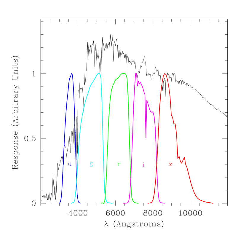
Figure 1: Estimated response for all five bands in the SDSS (accounting for the atmosphere, the mirrors, the filters, and the CCDs), as a function of observed wavelength, as measured by Mamoru Doi. The predicted spectrum $f(\lambda)$ for a 4 Gyr old instantaneous burst using the models of Bruzual & Charlot (1993) (and observed at $z=0$) is shown for reference.

The response functions $R(\lambda)$ of the filter-CCD combinations have been measured using a monochrometer by Mamoru Doi. Using a model for the atmospheric transmission and the reflectivity of the primary and secondary mirrors, one can then model the response of the entire system. For each bandpass in the SDSS, there are six different CCDs; it has been shown that the differences are small between these CCD and filter responses for each bandpass. The resulting set of filter curves is shown in Figure 1, in comparison to a model of a galaxy spectral energy distribution observed at $z=0$ (a 4 Gyr old instantaneous burst from the models of Bruzual & Charlot 1993).

The results of the spectroscopic observations are treated as follows. We extract one-dimensional spectra from the two-dimension images using a pipeline (specBS v4_8) created specifically for the SDSS instrumentation (Schlegel et al. 2002), which also fits for the redshift of each spectrum. The official SDSS redshifts are obtained from a different pipeline (SubbaRao et al. 2002). The two independent versions provide a consistency check on the redshift determination, and for galaxies they agree on more than 99% of the objects.

We use two types of magnitudes determined by the SDSS. First, the SDSS Petrosian magnitudes, a modified form of the magnitude described by Petrosian (1976), as described in Strauss et al. (2002). Petrosian magnitudes are circular aperture magnitudes with an aperture size which is determined by the shape of the radial profile (not its amplitude). The resulting apertures are empirically nearly constant in metric size as a function of redshift; in addition, all the bands use the same aperture, so the measured SED corresponds (to within the effects of seeing) to the SED of an identifiable region of the galaxy. However, for faint objects, the Petrosian magnitudes tend to become noisy. Thus, for galaxies with $z>0.25$ we instead use the higher signal-to-noise “model magnitudes.” Model magnitudes are calculated in all bands using a single weighted aperture convolved with the point spread function; thus, the measured colors again correspond to an identifiable region of the galaxy, though a different one than would be measured by the Petrosian magnitude. The weighted aperture is the better fitting model (pure exponential or pure de Vaucouleurs) to the galaxy image in the $r$-band. Thus, the model magnitudes weight the centers of galaxies more strongly than do Petrosian magnitudes. In Stoughton et al. (2002) we are explicitly warned not to mix Petrosian and model magnitudes in a single analysis, since they measure galaxies in very different ways. Nevertheless, for the purposes of contraining galaxy template SEDs, it is perfectly acceptable to use any well-defined part of any galaxy. For our purposes, it is more important to have high signal-to-noise measurements of galaxy colors than to measure exactly the same regions of galaxies at low and high redshift. We extinction-correct both types of magnitudes using the dust maps of Schlegel, Finkbeiner & Davis (1998).

3.2 Fitting SEDs to SDSS Data

For the purposes of using the SDSS data to constrain our template set, we take a subsample of the data consisting of around 30,000 objects in the range $0.0<z<0.5$. The sample includes both the main sample and the LRGs, and is designed such that there is an approximately even distribution over redshift within our range of redshifts. In addition, we add results from galaxies in several spectroscopic plates (totalling about 1,000 objects) which were selected by a photometric redshift algorithm (Csabai et al., in preparation) to be at around $z\sim 0.3$–$0.4$, and subsequently observed spectroscopically. These objects are invaluable for tying down the blue end of the templates. Finally, we exclude galaxies in the redshift range $0.28<z<0.32$ from the fit for the templates, for reasons which we will explain more fully below (nevertheless, we still can and do use the resulting templates to analyze galaxies in this range).

Some of the objects have missing or poorly constrained data. For example, the $u$- or $z$-band fluxes for some objects are swamped by the photon noise of the sky. We identify such cases as magnitude errors greater than 2.0 or magnitudes fainter than 24.0 in any band. We ignore these objects entirely when fitting for the templates.

In addition, the photometric errors for most objects in the spectroscopic galaxy sample of the SDSS are not dominated by the estimated errors on the photometry listed in the catalog. Instead, the errors are dominated by local calibration errors and other systematic effects, which are poorly known. To account for these errors, we add extra error terms in quadrature with the errors listed in the catalog (0.05 mags, 0.02 mags, 0.02 mags, 0.02 mags, and 0.03 mags for $ugriz$, respectively). The choice of these values is based on a qualitative sense of the photometric errors present in the data. Not accounting for this extra source of errors can cause the fits to be ill-behaved.

For the SED space (our ${\bf v}_{i}(\lambda)$), we use the subspace defined by ten Bruzual-Charlot instantaneous burst models with ages ranging from $3\times 10^{7}$ to $2\times 10^{10}$ years, five with metallicity $Z=0.02$ and five with $Z=0.004$, all assuming a Salpeter Initial Mass Function. Since we cannot recover information about the SED below a certain wavelength resolution, we smooth most of the wavelength regime of the templates using a Gaussian with a standard deviation of $\sigma=300$Å; for the region of the spectrum which contains the sharpest gradients, around 4000Å, we smooth only with $\sigma=150$Å. None of our results change dramatically if we vary our smoothing procedure or if we add reddened templates to our allowed SED space.

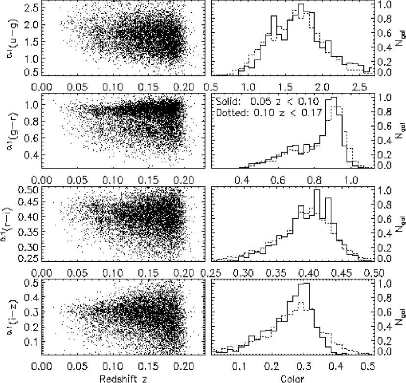
Figure 6: Similar to Figure 5, but now the colors are $K$-corrected to $z=0.1$. There is very little dependence of the colors on redshift, even for the ${}^{{0.1}}\!{u}$ band, where the low-redshift end is an extrapolation of the data.

We choose to fit for $N_{t}=4$ eigentemplates, the maximum one can use and still allow freedom to fit for the templates themselves. Simply using five templates (which obviously reproduces all the magnitudes exactly) tends to yield unphysical trends of galaxy SED versus redshift (cf. Figure 6 below). Using three templates does nearly as well as four templates in the sense that the resulting templates reproduce the $griz$ magnitudes nearly as well. However, the fourth template is necessary to recover the $u$-band flux to better than about 15%. In addition, since one of the applications of these SED determinations is the distribution of galaxy colors in fixed frame magnitudes, we don’t want to artificially reduce the dimensionality of the color space to only two.

One more choice needs to be made, the wavelength regime over which to orthogonalize the templates and over which to calculate the flux. We choose the range defined by $\lambda_{\mathrm{min}}=3500$Å and $\lambda_{\mathrm{max}}=7500$Å, since this rest frame range is observed for almost all galaxies in the sample. We refer here and in other papers to the flux and luminosity in this range as the “visual flux” $f_{v}$ and the “visual luminosity” $L_{v}$.

Once we have finished fitting for the templates, we still want to determine a best-fit SED for each object. Thus, after the templates have been determined, we fit for the coefficients $a_{i}$ for each galaxy, including those excluded from the template-fitting procedure because of large errors. In order to accommodate the presence of errors, we constrain all the SED fits to all galaxies using the method described in Section 2.2. As a constraint, we use the covariance matrix and mean value (essentially zero, by design) of the coefficients of the well-measured set of galaxies used to determine the templates; we multiply all the elements of the covariance matrix by a factor of four to weaken our constraint (which is appropriate, since the actual distribution of coefficients is not well described by a single gaussian). Thus, we account for any missing information by simply requiring that the object SED have “reasonable” properties. The constraint does not affect the results for galaxies which have well-measured magnitudes in all bands.

3.3 The $g$/$r$ Gap

In Figure 1, there is clearly a gap between the $g$ and $r$ bands. Linear fits to the data allow considerable freedom in the resulting reconstructed SEDs. As it happens, one of the directions in our best fit coefficient space $a_{i}/a_{0}$ corresponds to a large spike at around 4000 Å; that this direction is important is not surprising, since one of the most variable quantities of galaxy SEDs is the size of the 4000 Å break. However, the gap between the $g$ and $r$ bands corresponds to the 4000 Å break at around $z=0.3$. The existence of this spike in one direction in our four-dimensional space means that galaxies at $z=0.3$ can vary along this direction in order to better fit $u$, $i$, and $z$, with little effect on the $g-r$ color of the fit. This results in unphysical SED fits to galaxies near $z=0.3$. One really only needs to worry about this effect in the SDSS when one is dealing with the LRGs, for galaxies in the range about $0.27<z<0.33$. The Main Sample results are not significantly affected at all (since few Main Sample galaxies are at $z>0.25$. Furthermore, one can still observe a galaxy at $z=0.1$ and reliably infer what it would look like at $z=0.3$; it is only the reverse process which is difficult.

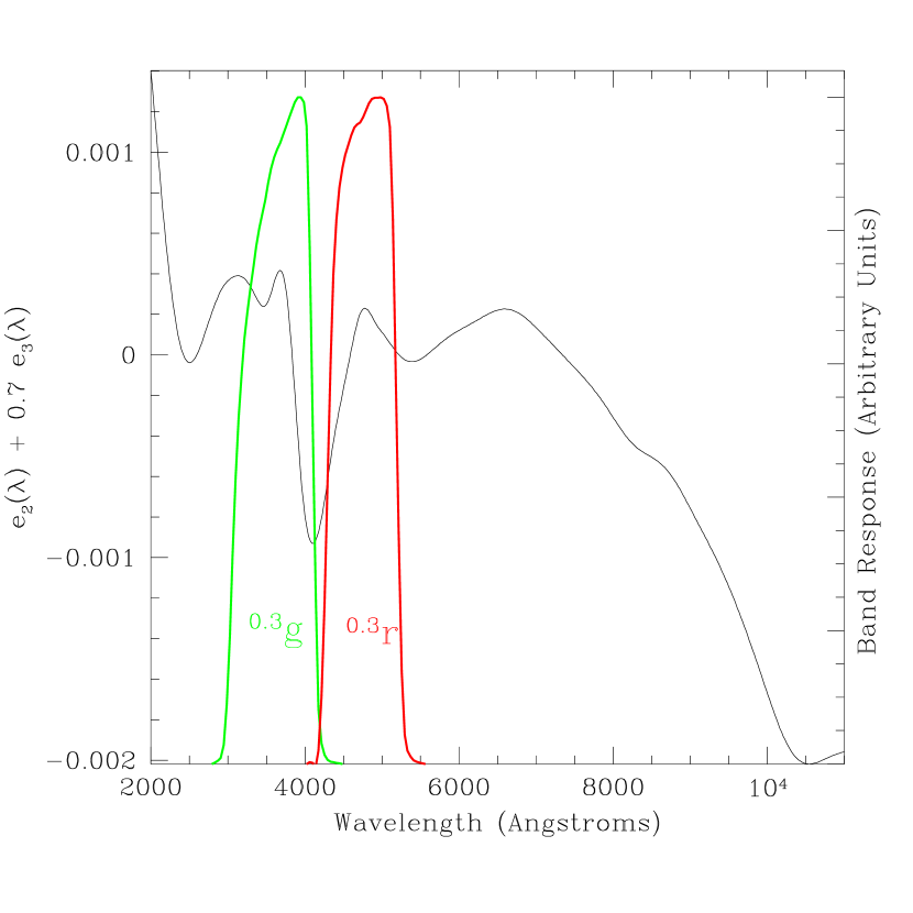
Figure 2: The spectrum corresponding to the direction of the spur in the upper right panel of Figure 3. Note the strong feature near 4000 Å. Overplotted are the bandpasses for ${}^{{0.3}}\!{g}$ and ${}^{{0.3}}\!{r}$. The strong features fall in the gap between the bandpasses. Thus, in a linear fit to a galaxy at $z=0.3$, this component can be used to fit the observed magnitudes without being constrained to have reasonable behavior around 4000 Å.

To demonstrate this degeneracy, Figure 2 shows the spectrum corresponding to the direction represented by the vector ${\bf e}_{2}+0.7{\bf e}_{3}$, for our best fit templates. We overplot the ${}^{{0.3}}\!{g}$ and ${}^{{0.3}}\!{r}$ bands. This direction has a strong peak in the gap between the two bands at $z=0.3$. This difficulty is why, in Section 3, we exclude the regime around $z\sim 0.3$; otherwise the templates became distracted by the degeneracies in this range.

We have explored using a larger set of input spectra, by including reddened versions of all our templates, to test whether a more complete space of SEDs would cause our fit to choose a more realistic subspace. In addition, we have tried removing the increased resolution of the template SEDs around the 4000 Å break. Neither of these tests yielded better results.

Our opinion is that the ideal regularization which would solve this problem would be to minimize $\chi^{2}$ under the constraint that none of the original Bruzual-Charlot spectra defining our SED space contribute negatively to the SED fit. Such a solution would almost certainly have better properties than our linear approach here: it would almost certainly avoid the degeneracies, it would yield reasonable fit SED over a larger wavelength range, it would associate a reasonable star-formation history with each object (which could be used to evolution-correct the magnitudes).

However, we have not tackled this approach yet. As it happens, the direct constraint on the coefficients described in the previous section is sufficient to suppress the $g$/$r$ gap problem for many purposes, as long as one $K$-corrects the magnitudes to $z=0.3$. In this way, one minimizes the $K$-corrections for the galaxies which one is least certain of.

3.4 Results

The top two panels of Figure 3 show the pairwise joint distributions of $a_{1}/a_{0}$, $a_{2}/a_{0}$, and $a_{3}/a_{0}$ for a random subset of about 10,000 of the galaxies in the SDSS sample (not only the ones which we used to fit the templates). In the bottom panel, three spectra taken from a one-dimensional sequence along the galaxy locus are shown, showing that the spectra become progressively bluer along that sequence. Note that constraints on the SED become poor at the bluest and reddest edges of this diagram (the peak of the $z$-band response is at 8700 Årest frame for a galaxy observed at $z=0$). Therefore, the odd behavior near the edges should not be taken too seriously. In addition, note the small spur extending from lower left to upper right through the right edge of the ($a_{3}/a_{0}$)-($a_{2}/a_{0}$) plane. Many of the objects in this spur are at around $z=0.3$, and this spur is the result of the degeneracy due to the $g$/$r$ gap.

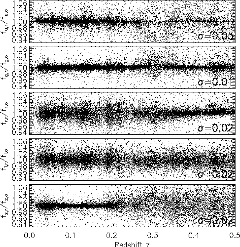
Figure 4: Reconstructed galaxy fluxes relative to the observed galaxy fluxes, for all five SDSS bands, shown for a random subsample consisting of around 10,000 of the SDSS galaxies. The residuals are shown against redshift. There is no systematic trend with redshift in any band. The 5-$\sigma$ clipped estimate of the scatter around the observed fluxes is listed for each band. In $u$, $g$, $r$, and $i$ the scatter is consistent with the expected photometric errors in the survey at all redshifts. At high redshift the scatter in $z$ becomes large, most likely due to increasing photometric errors.

These reconstructed spectra do an excellent job of reproducing the observed galaxy fluxes. Figure 4 shows the differences between the observed and reconstructed fluxes as a function of redshift. There are no systematic trends with redshift, and the standard deviations of the differences between the observed and the reconstructed fluxes (shown on the right bottom corner of each panel) are of order the photometric errors in the sample. In particular, for our 30,000 galaxies (and thus approximately 30,000 degrees of freedom) we find $\chi^{2}\sim 55,000$, indicating that our fit is reasonable.

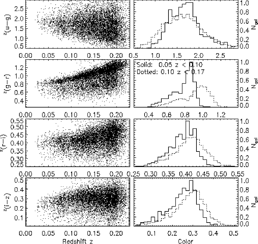
Figure 5: Color distributions in the observed frame for SDSS Main Sample galaxies in the luminosity range $-21.5<M_{{}^{{0.1}}\!{r}}<-21.2$. This sample is complete (that is, volume limited) for $0.05<z<0.17$. Left panels show the colors as a function of redshift. Right panel shows the distributions of each color at high and low redshift within the volume-limited subsample. The observed colors clearly depend strongly on redshift.

An important test of the consistency of the fits is to check that for a fixed type of galaxy, the distribution of the fixed frame colors depends only weakly on redshift. Because the galaxies shown in Figures 3 and 4 are inhomogeneously selected — some are Main Sample galaxies, some are LRGs, and some are selected from the photometric redshift plates — we will split our sample into two well-defined sets of objects to perform this test. First, we choose a set of Main Sample galaxies in the luminosity range $-21.5<M_{{}^{{0.1}}\!{r}}<-21.2$. Figure 5 shows the observed-frame colors of all the galaxies as a function of redshift. The right-hand panels show the distribution for redshifts $0.05<z<0.10$ (solid histogram) and $0.10<z<0.17$ (dotted histogram). A trend exists in all colors, most strongly in ${}^{{z}}\!{(g-r)}$. Figure 6 shows the $K$-corrected colors ${}^{{0.1}}\!{(u-g)}$, ${}^{{0.1}}\!{(g-r)}$, ${}^{{0.1}}\!{(r-i)}$, and ${}^{{0.1}}\!{(i-z)}$ in the same manner. The plots show a general consistency in the fixed frame color distribution of these objects with redshift. Small changes are discernible in the distributions, mostly attributable to the increased errors at higher redshift. Note that for $z<0.1$ the ${}^{{0.1}}\!{(u-g)}$ color depends on an extrapolation of the SED in the blue, while for $z>0.1$ the ${}^{{0.1}}\!{(i-z)}$ color depends on an extrapolation of the SED in the red.

Second, we choose a set of Cut I LRGs (see Eisenstein et al. 2001 for details) with $-22.8<M_{{}^{{0.3}}\!{r}}<-22.5$. Figure 7 shows the observed colors as a function of redshift for these objects. Again, there is a strong redshift dependence. Figure 8 shows the colors $K$-corrected to $z=0.3$, which appear approximately constant with redshift. ${}^{{0.3}}\!{(g-r)}$ (which is very similar to ${}^{{0.0}}\!{(u-g)}$) experiences a blueward shift of about 0.1 magnitudes between $z=0.1$ and $z=0.45$, which is attributable to passive evolution, though it could also be due to the LRG selection procedure.

In short, these fits to galaxy SEDs provide estimates which reproduce the galaxy photometry nearly to the level of the errors in the photometry itself, seem physically reasonable, and are consistent over the range of redshifts we consider ($0.0<z<0.5$).

3.5 $K$-corrections in the SDSS

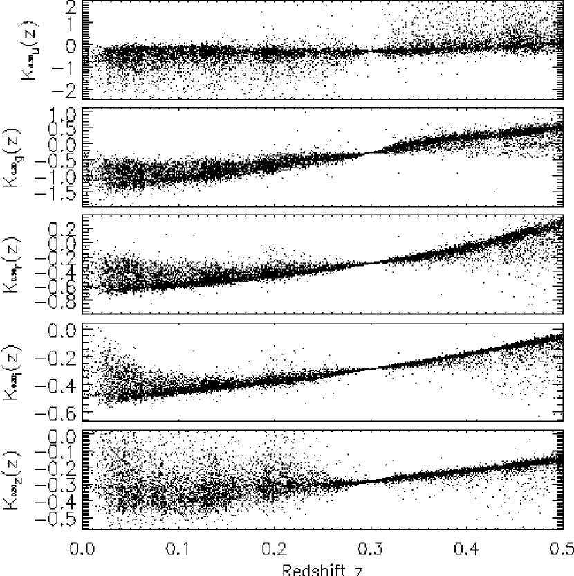
Figure 9: $K$-corrections to $z=0.3$ as a function of redshift in all five bands for a random subsample consisting around 10,000 of the SDSS galaxies. The range of $K$-corrections at each redshift reflects the range of galaxy types at each redshift. The $K$-corrections are largest, and therefore the most uncertain, for the ${}^{{0.3}}\!{u}$ and ${}^{{0.3}}\!{g}$ bands. While we show the $K$-corrections for ${}^{{0.3}}\!{u}$ at $z<0.3$ and for ${}^{{0.3}}\!{z}$ at $z>0.3$, and indeed these $K$-corrections are fairly well-behaved, we do not recommend using these extrapolated results for scientific purposes.

We show, in Figure 9, the resulting $K$-corrections to $z=0.3$ inferred from this method, for all five SDSS bands. Note that the $K$-corrections are largest (and thus most uncertain) in ${}^{{0.3}}\!{u}$ and ${}^{{0.3}}\!{g}$. Remember that the $K$-corrections to ${}^{{0.3}}\!{u}$ are extrapolations for $z<0.3$ and that the $K$-corrections to ${}^{{0.3}}\!{z}$ are extrapolations for $z>0.3$, so those results should not be taken too seriously. (Although the $K$-corrections given are not too unreasonable).

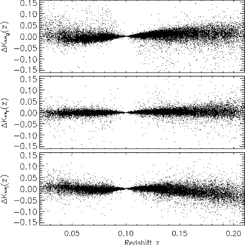
Figure 10: Difference between the $K$-corrections to $z=0.1$ determined from the spectroscopy and those determined from the analysis of broad-band magnitudes synthesized from the same spectra.

An important test of our method is to synthesize broad band photometry from spectra, and then try to recover the $K$-corrections in a case where we know the spectrum completely. For this purpose, we use as example spectra the spectra of galaxies in the SDSS. Since we cannot synthesize the observed $u$ and $z$ bands from these spectra, we simply base them on the synthesized $g$ and $i$ band magnitudes plus the actual $u-g$ and $z-i$ colors. (This procedure is unlikely to make the photometric estimations of the $K$-corrections better). Finally, we added 2% random errors to all of the measurements. Figure 10 compares the $K$-corrections from the synthesized photometry to that calculated from the spectrum itself:

$$\Delta K=K_{\mathrm{spec}}-K_{\mathrm{photo}}$$ (14)

Since all of the photometry used in this test is actually synthesized from the spectra, this is not a comparison of photometric and spectroscopic $K$-corrections; it is only a test of how well our method recovers $K$-corrections. The agreement in FIgure 10 is very good, suggesting that our method can indeed recover the correct $K$-corrections based only on broad band magnitudes.

To test how robust these $K$-correction results are to our model assumptions, we compare them to other methods of calculating fixed frame galaxy magnitudes. An extremely simple method is to calculate the flux in any desired bandpass by fitting a power-law slope and amplitude to the fluxes in the two adjacent bandpasses (extrapolating when necessary). Figure 11 shows the differences in the $K$-corrections inferred from this method and those inferred from the method of Figure 9, as a function of redshift. $r$, $i$, and $z$ are all reasonably similar in either method; $u$ and $g$, however, have distinct trends with redshift, mostly due to the non-power law nature of the template galaxy spectra (and probably actual galaxy spectra) in this regime. To show this fact, we perform a similar power-law fit, only this time including a break in the spectrum at 4000 Å. We use the $u$-$g$ color to fit the break, assuming that the slope blueward of 4000 Å is $f(\lambda)\propto\lambda^{2}$. Figure 12 shows the results of this fit; the redshift trend in $g$ is greatly reduced, as is the trend in $u$, but a large amount of scatter remains in the $u$ band. This results from the fact that you can either fit the slope of the SED below the 4000 Å break or the size of the 4000 Å break itself; it is not possible with this data to constrain both in an individual spectrum, which is a limitation of our determination of fixed frame $u$-band magnitudes.

Finally, it is possible to use the galaxy spectra obtained with the spectrograph to estimate the $K$-correction for each object. However, this procedure requires trusting the spectrophotometry over a wide wavelength range. In addition, the region of the galaxy which the spectra cover is not completely well defined. The small scale wavelength features are set by the fiber aperture ($3^{\prime\prime}$ in diameter) while large scale wavelength features are constrained by a short “smear exposure” which covers a larger area. The smear exposure corrections are clearly the correct approach for point sources, but for galaxies it causes the small scale and large scale features of the spectrum to be determined by somewhat different regions of the galaxy.

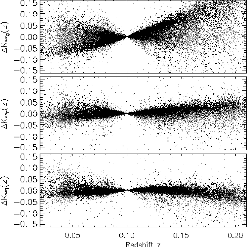
Figure 13: Difference between the $K$-corrections to $z=0.1$ determined from the spectroscopy and those determined from the analysis of the broad-band Petrosian magnitudes, for Main Sample galaxies.

Nevertheless, in Figure 13, we compare the $K$-corrections to $z=0.1$ of Main Sample galaxies calculated based on the spectra to those of Figure 9, finding that they are quite similar. There is a trend with redshift in the $g$-band, which is due to the fact that on average the $g-r$ color is about 0.1 magnitudes redder in the fiber aperture than in the Petrosian aperture. The implication is that the $K$-corrections are stronger for the aperture which corresponds to the spectrum than for the Petrosian aperture. This indicates that for work which requires precision, it is best to avoid using the $K$-corrections determined from the spectra. (Note that in the second paragraph of this section we used the SDSS spectra as example spectra to validate the method as applied to synthesized photometry; in this paragraph we have evaluated whether to rely on fiber spectra to calculate $K$-corrections for the Petrosian photometry).

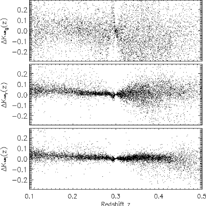
Figure 14: Difference between the $K$-corrections to $z=0.3$ determined from the spectroscopy and those determined from the analysis of the broad-band model magnitudes, for LRGs.

For completeness, Figure 14 compares the spectroscopic and photometric $K$-corrections to $z=0.3$ of LRGs. The ${}^{{0.3}}\!{r}$ and ${}^{{0.3}}\!{i}$ bands agree very well. However, there is considerable scatter in the ${}^{{0.3}}\!{g}$ band (nearly equivalent to the ${}^{{0.0}}\!{u}$ band), at around 20%. Because the LRGs tend to have small color gradients, the issues of fiber sizes and smear exposures are not important in this context.

4 Conclusions and Future Work

We have presented a method and an implementation for estimating galaxy SEDs for the purpose of calculating fixed frame galaxy magnitudes over a range of redshifts. We have demonstrated that it gives sensible and consistent results. We will be using this method in future papers which will describe the joint distribution of luminosities and colors of galaxies, as well as the evolution of the luminosity function of galaxies. Furthermore, we plan to incorporate observations of objects in bands other than the SDSS bands to further describe the nature of galaxy SEDs.

We have not discussed in detail the question of error analysis. There is no answer to this question which is simple, general, and realistic. The photometric errors can of course be propagated to the errors on the reconstructed magnitudes, but these estimates do not describe the errors associated with the restriction to a three-dimensional space of SED shapes. An idea of the level of errors can be gleaned from the comparison of our method to other methods of $K$-correction. Clearly, $r$, $i$ and $z$ can be reconstructed to the level of the photometry. Judging from Figure 10, the $g$ band can be reconstructed to about 5% accuracy. The $u$ band is more difficult to evaluate. Judging from the poor reconstructions of the ${}^{{0.3}}\!{g}$ band (nearly equal to the ${}^{{0.0}}\!{u}$ band, the reconstructions may be as bad as 20% accuracy.

Topics we have not discussed here are dust- and evolution-correction of the magnitudes. Some of the scatter in the three-dimensional space describing the shape of the galaxy SED is probably due to dust. It may be possible to evaluate the effects of reddening in this space and, by assuming that galaxies corrected for internal reddening live in an even lower dimensional space, perform a reddening correction. We will be investigating this question in the near future. One can perform a similar exercise with evolution estimates, relating the position of a galaxy along the $a_{1}$ axis in Figure 3 to a particular star-formation history, and estimating the evolution of the object from that history.

The distribution of galaxies in the three-dimensional space of galaxy SEDs described here may be useful for other purposes, as well. For example, you can calculate photometric redshifts using the method described here. kcorrect v1_11 has a simple (and very fast) photometric redshift estimator with very tight core of residuals ($\sigma\sim 0.05$) in a comparison to SDSS galaxies with redshifts. However, we warn the reader that before this code can be used as a reliable photometric redshift indicator, more work has to be done (which the reader is invited to do using the released code) to identify galaxies which are likely to be redshift outliers and to handle galaxies at $z>0.5$ (which have photometric observations which are bluer in the rest frame than for any galaxies in our training set). Until this method is perfect and our templates are better constrained, we recommend the photometric redshift method and results of Csabai et al., in preparation. Another use of the three-dimensional space of galaxy SEDs is to create mock samples of galaxies observed in any bandpass at any redshift. We are working on quantifying the correlations between these coefficients and luminosity, surface-brighntess and radial profile in order to create mock catalogs which truly reflect the correlations between galaxy properties found in the data.

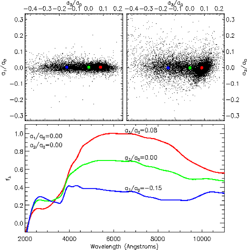
Figure 3: Top panels: Distribution of the components of the four-parameter fit to the five-band SDSS photometry for a random subsample consisting of 10,000 of the SDSS galaxies. $a_{0}$ is linearly proportional to the flux between 3500 Åand 7500 Å, while $a_{1}$, $a_{2}$, and $a_{3}$ contribute no flux in this range. Thus, the ratios $a_{1}/a_{0}$, $a_{2}/a_{0}$, and $a_{3}/a_{0}$ describe the spectral type of the galaxy. $a_{3}/a_{0}$ is the most variable parameter and thus is the best separator of galaxy type. The spur extending from the lower left to the upper right from the red dot in the $(a_{3}/a_{0})$-$(a_{2}/a_{0})$ plane is due to a degeneracy for galaxies at $z\sim 0.3$, described in detail in Section 3.3. Bottom panel: At fixed $a_{1}/a_{0}$ and $a_{2}/a_{0}$, the inferred spectra corresponding to various values of $a_{3}/a_{0}$. Near $a_{3}/a_{0}=-0.20$, the spectrum is similar to that of an elliptical galaxy. For higher values, the spectrum becomes bluer.

Figure 7: Similar to Figure 5, now showing LRG galaxies (Cut I) in the luminosity range $-22.8<M_{{}^{{0.3}}\!{r}}<-22.5$. Again, there is a strong dependence on redshift.

Figure 8: Same as Figure 7, now $K$-correcting the LRG galaxies to $z=0.3$. The redshift dependence is greatly reduced for the LRGs in comparison to Figure 7; on the other hand, there are distinct trends of restframe color with redshift. In ${}^{{0.3}}\!{(g-r)}$ an overall trend is apparent; LRGs at $z=0.4$ are about 0.1 magnitudes bluer than LRGs at $z=0.2$. A change of this magnitude is attributable to passive galaxy evolution, though considerably more work needs to be done to show that this is occurring. In ${}^{{0.3}}\!{(r-i)}$, a blueward shift also occurs, though at a much smaller level.

Figure 11: Difference in the $K$-corrections to $z=0.1$ in each band between the method used in Figure 9 and the method of simply interpolating between adjacent bands fitting a power-law SED. The differences are small in ${}^{{0.1}}\!{r}$, ${}^{{0.1}}\!{i}$, and ${}^{{0.1}}\!{z}$, where galaxy SEDs have simple shapes. There are large systematic differences in ${}^{{0.1}}\!{u}$ and ${}^{{0.1}}\!{g}$, for which the 4000 Å break is important in the spectral templates used.

Figure 12: Same as Figure 11, now comparing to a method of interpolating the bandpasses using power-laws, and fitting for the 4000 Å break. The systematic trends in ${}^{{0.1}}\!{u}$ and ${}^{{0.1}}\!{g}$ are gone (though there is considerable scatter in ${}^{{0.1}}\!{u}$).

References

- Binney & Merrifield (1998) Binney, J., & Merrifield, M. 1998, Galactic Astronomy (Princeton: Princeton University Press)
- Bruzual & Charlot (1993) Bruzual, A. G., & Charlot, S. 1993, ApJ, 405, 538
- Budávari et al. (2000) Budavári, T.; Szalay, A. S.; Connolly, A. J.; Csabai, I.; Dickinson, M. (2000), AJ, 120, 1588
- Csabai et al. (2000) Csabai, I., Connolly, A. J., Szalay, A. S., & Budavári, T. 2000, AJ, 119, 69
- Eisenstein et al. (2001) Eisenstein, D. J., et al. SDSS Collaboration 2001, 122, 2267
- Fan (1999) Fan, X. 1999, AJ, 117, 2528
- Frei & Gunn (1994) Frei, Z., & Gunn, J. E. 1994, AJ, 108, 1476
- Fukugita et al. (1996) Fukugita, M., Ichikawa, T., Gunn, J. E., Doi, M., Shimasaku, K., & Schneider, D. P. 1996, AJ, 111, 1748
- Fukugita, Shimasaku, & Ichikawa (1995) Fukugita, M., Shimasaku, K., & Ichikawa, T. 1995, PASP, 107, 945
- Gunn et al. (1998) Gunn, J. E., Carr, M. A., Rockosi, C. M., Sekiguchi, M., et al. 1998, AJ, 116, 3040
- Hogg (1999) Hogg, D. W. 1999, astro-ph/9905116
- Oke & Gunn (1983) Oke, J. B., & Gunn, J. E. 1983, ApJ, 266, 713
- Oke & Sandage (1968) Oke, J. B., & Sandage, A. 1968, ApJ, 154, 21
- Petrosian (1976) Petrosian, V. 1976, ApJ, 209, L1
- Press et al. (1992) Press, W. H., Teukolsky, S. A., Vetterling, W. T., & Flannery, B. P. 1992, Numerical Recipes (Cambridge: Cambridge Univ. Press)
- Schlegel, Finkbeiner & Davis (1998) Schlegel, D. J., Finkbeiner, D. P., & Davis, M. 1998, ApJ, 500, 525
- Schlegel et al. (2002) Schlegel, D. J., et al. 2002, in preparation
- Smith et al. (2002) Smith, J. A., et al. SDSS Collaboration 2002, AJ, 123, 2121
- Stoughton et al. (2002) Stoughton, C., et al. 2002, AJ, 123, 485
- Strauss et al. (2002) Strauss, M. A., et al. 2002, submitted to AJ
- SubbaRao et al. (2002) SubbaRao, M., et al. 2002, in preparation
- York et al. (2000) York, D., et al. 2000, AJ, 120, 1579