The Physical Properties of the Ly$\alpha$ Forest at $z>1.5$^,

Abstract

Combining a new, increased dataset of 8 QSOs covering the Ly$\alpha$ forest at redshifts $1.5<z<3.6$ from VLT/UVES observations with previously published results, we have investigated the properties of the Ly$\alpha$ forest at $1.5<z<4$. With the 6 QSOs covering the Ly$\alpha$ forest at $1.5<z<2.5$, we have extended previous studies in this redshift range. In particular, we have concentrated on the evolution of the line number density and the clustering of the Ly$\alpha$ forest at $z\leq 2.5$, where the Ly$\alpha$ forest starts to show some inhomogeneity from sightline to sightline. We have fitted Voigt profiles to the Ly$\alpha$ absorption lines as in previous studies, and have, for two QSOs with $z_{\mathrm{em}}\sim 2.4$, fitted Ly$\alpha$ and higher order of Lyman lines down to 3050 Å simultaneously. This latter approach has been taken in order to study the Ly$\beta$ forest at $z\sim 2.2$ and the higher H i column density Ly$\alpha$ forest in the Ly$\beta$ forest region.

For a given $N_{\mathrm{H\,\mathsc{i}}}$ range, the Ly$\alpha$ forest at $1.5<z<4$ shows the monotonic evolution, which is governed mainly by the Hubble expansion at this redshift range. In general, the Ly$\alpha$ forest line number density ($dn/dz$) is best approximated with $dn/dz=6.1\,(1+z)^{2.47\pm 0.18}$ for the H i column density $N_{\mathrm{H\,\mathsc{i}}}=10^{13.64-17}\ {\mathrm{cm}}^{-2}$ at $1.5<z<4$. When the results at $0<z<1.5$ from HST observations are combined, the slow-down in the number density evolution occurs at $z<1.5$. For higher column density clouds at $N_{\mathrm{H\,\mathsc{i}}}>10^{14}\ {\mathrm{cm}}^{-2}$, there is a variation in the line number density from sightline to sightline at $z<2.5$. This variation is stronger for higher column density systems, probably due to more gravitationally evolved structures at lower $z$. The mean H i opacity $\overline{\tau}_{\mathrm{H\,\mathsc{i}}}$ is $\overline{\tau}_{\mathrm{H\,\mathsc{i}}}(z)=0.0032\,(1+z)^{3.37\pm 0.20}$ at $1.5<z<4$. HST observations show evidence for slower evolution of $\overline{\tau}_{\mathrm{H\,\mathsc{i}}}$ at $z<1$. For $N_{\mathrm{H\,\mathsc{i}}}=10^{12.5-15}\ {\mathrm{cm}^{-2}}$, the differential column density distribution function, $f(N_{\mathrm{H\,\mathsc{i}}})$, can be best fit by $f(N_{\mathrm{H\,\mathsc{i}}})\propto N_{{\mathrm{H\,\mathsc{i}}}}^{-\beta}$ with $\beta\approx 1.5$ for $1.5<z<4$. When combined with HST observations, the exponent $\beta$ increases as $z$ decreases at $0<z<4$ for $N_{\mathrm{H\,\mathsc{i}}}=10^{13-17}\ {\mathrm{cm}^{-2}}$. The correlation strength of the step optical depth correlation function shows the strong evolution from $<\!z\!>\ =3.3$ to $<\!z\!>\ =2.1$, although there is a large scatter along different sightlines. The analyses of the Ly$\beta$ forest at $z\sim 2.2$ are, in general, in good agreement with those of the Ly$\alpha$ forest.

1 Introduction

The redshift evolution of the Ly$\alpha$ forest imprinted in the spectra of high-$z$ QSOs provides a powerful tool to probe the distribution and evolution of baryonic matter, and hence the formation and evolution of galaxies and the large scale structure, over a wide range of redshifts up to $z\sim 6$ (Sargent et al. 1980; Schaye et al. 1999; Kim, Cristiani & D’Odorico 2001, hereafter KCD).

The evolution of the Ly$\alpha$ forest is mainly governed by two physical processes. One is the Hubble expansion and another is the ionizing ultraviolet background flux (Theuns, Leonard & Efstathiou 1998; Davé et al. 1999; Schaye et al. 2000; Bianchi, Cristiani & Kim 2001). At higher $z$, the Hubble expansion and the non-decreasing ultraviolet background cause a rapid evolution of the line number density per unit redshift, $dn/dz$. At lower $z$, the number of photons available to ionize the Ly$\alpha$ forest becomes smaller, due to the decrease of the number of QSOs at $z<2$, which is generally assumed to be the main source of the ionizing photons. As a result the rate of change of $dn/dz$ with redshift is smaller.

Studies on the forest at $z>2$ have shown the rapid evolution of the line number density (Lu, Wolfe & Turnshek 1991; Bechtold 1994; Kim et al. 1997; KCD). Weymann et al. (1998) from the HST QSO absorption line key project, however, have shown that the redshift evolution of the line number density is much more gradual at redshifts below $z\sim 1.5$ than above. These results suggest that the transition between the two different evolutionary rates occur somewhere in the range $z\sim 1.3\to 1.7$. From numerical simulations, Theuns et al. (1998) and Davé et al. (1999) have demonstrated that the change in the evolutionary slope occurs at $z\sim 1.7$ due to the decreasing UV background at $z<2$, assuming a QSO-dominated background. Recently, from the study of the Ly$\alpha$ forest at $1.5<z<2.4$, KCD conclude that the Ly$\alpha$ forest at $1.5<z<4$ shows a monotonic, continuous evolution with $z$, in terms of the line number density, the mean H i opacity and the correlation strength, both from the profile fitting analysis and from the optical depth analysis. KCD also show that the change in the number density evolution occurs at $z\sim 1.2$, suggesting that a QSO-dominated UV background used in numerical simulations underestimates the UV background and/or the enhanced structure formation at $z<2.5$ (Theuns et al. 1998; Weymann et al. 1998; Davé et al. 1999; Bianchi et al. 2001). Therefore, it is of importance to investigate the redshift range where $dn/dz$ starts to change and to study any variations from sightline to sightline from larger statistical sample in order to constrain the results from numerical simulations and the nature of the ionizing sources.

Here, we present the analysis of six QSOs covering the Ly$\alpha$ forest at $1.5<z_{\mathrm{Ly\alpha}}<2.4$ as well as two QSOs at $3<z_{\mathrm{Ly\alpha}}<3.6$ from high resolution ($R\sim 45\,000$), high S/N ($\sim$ 35–50) spectra obtained with the VLT/UVES. This analysis is an extension of the one by KCD with a larger uniform sample. We consider the evolutionary behavior of the Lyman forest systems over the redshift range $1.5<z<2.4$, in particular the line number density evolution and the clustering, and compare the results with those found by others at higher and lower redshifts. We have adopted the traditional Voigt profile fitting method to analyse the absorption lines in two ways. In the first approach, we have fitted the Ly$\alpha$ forest region using the Ly$\alpha$ lines only, since most previous studies have adopted this approach. In the second approach, we have fitted the Ly$\alpha$ forest with the higher order lines of Lyman series (predominantly Ly$\beta$) at wavelengths down to the observational limit, 3050 Å, for two QSOs at $z_{\mathrm{em}}\sim 2.4$ among 8 QSOs presented in this study. This analysis includes the Ly$\alpha$ forest from lower $z$ in the regions where these higher order lines are present. In Section 2, we describe the UVES observations, data reduction and the Voigt profile fitting. In Section 3, we present the analysis of the Ly$\alpha$ forest from the fitted line parameters, such as the number density. The Ly$\beta$ forest region is discussed in Section 4. The conclusions are summarized in Section 5.

Table 1: Observation log

QSO	$B^{a}$	$z_{\mathrm{em}}$	Wavelength	Exp. time	Observing Date
			(Å)	(sec)
HE0515–4414	14.9	1.719	3050–3860	19000	Dec. 14, 18, 1999
Q1101–264	16.0	2.145	3050–3870	23400	Feb. 10–16, 2000
J2233–606	17.5	2.238	3050–3860	16200	Oct. 8-12, 1999
			3770–4980	12300	Oct. 10-16, 1999
HE1122–1648	17.7	2.400	3050–3870	26400	Feb. 10–16, 2000
			3760–4975	27000	Feb. 10–16, 2000
HE2217–2818	16.0	2.413	3050–3860	16200	Oct. 5–6, 1999
			3288–4522	10800	Sep. 27–28, 1999
HE1347–2457	16.8	2.617	3760–4975	18000	Feb. 10–16, 2000
Q0302–003	18.4	3.281	4806–5771	20000	Oct. 12–16, 1999
Q0055–269	17.9	3.655	4634–5600	18100	Sep. 20–22, 2000
			4790–5729	17000	Sep. 20–22, 2000

• Taken from the SIMBAD astronomical database. The magnitude of HE1347–2457 is from NED.

Table 2: Analyzed QSOs

QSO	$\lambda\lambda$	$z_{\mathrm{Ly\alpha}}$	$dX^{\mathrm{a}}$	# of linesb	$\overline{\tau}_{\mathrm{H\,\mathsc{i}}}$	$<\!z\!>$
Sample A
HE0515–4414	3080–3270	1.53–1.69	0.408	63	0.086${}^{0.049}_{-0.051}$	2.1
Q1101–264c	3230–3400	1.66–1.80	0.381	62	0.085${}^{0.049}_{-0.051}$
	3500–3778	1.88–2.08	0.685	99	0.106${}^{0.049}_{-0.051}$
	3230–3400, 3500–3778	1.66–2.08	1.066	161	0.096${}^{0.049}_{-0.051}$	2.1
J2233–606d	3400–3890	1.80–2.20	1.209	166	0.156${}^{0.049}_{-0.051}$	2.1
HE1122–1648	3500–4091	1.88–2.37	1.518	234	0.146${}^{0.049}_{-0.051}$	2.1
HE2217–2818	3510–4100	1.89–2.37	1.519	214	0.130${}^{0.049}_{-0.051}$	2.1
HE1347–2457	3760–4335	2.09–2.57	1.575	233	0.149${}^{0.049}_{-0.051}$	2.1
Q0302–003	4808–5150	2.96–3.24	1.152	167	0.334${}^{0.049}_{-0.051}$	3.3
Q0055–269	4852–5598	2.99–3.60	2.638	419	0.421${}^{0.049}_{-0.051}$	3.3
Q0000–263e	5450–6100	3.48–4.02	2.540	312	0.733${}^{0.049}_{-0.051}$	3.8
Sample B
HE1122–1648	3200–3500f	1.63–1.88	0.680		0.084${}^{0.049}_{-0.051}$
	3100–3500	1.55–1.88	0.893	21g
HE2217–2818	3200–3510f	1.63–1.89	0.704		0.142${}^{0.049}_{-0.051}$
	3100–3510	1.63–1.89	0.917	34g
The Ly$\beta$ forest
HE1122–1648	3674–4091	2.02–2.37	1.09	195
HE2217–2818	3674–4100	2.02–2.37	1.12	190

• For $q_{\mathrm{0}}=0$.

• Over the column density range, $N_{{\mathrm{H\,\mathsc{i}}}}=10^{12.5-17}\ {\mathrm{cm}}^{-2}$.

• There is a damped Ly$\alpha$ system at $z$ = 1.8386. The Ly$\alpha$ forest regions closer to the damped Ly$\alpha$ system by less than 50 Å at each side have been excluded in the study.

• See also Cristiani & D’Odorico (2000).

• Lu et al. (1996).

• For the spectral region 3100–3200 Å, the UVES spectra show a sharp decrease in S/N, so the continuum level is difficult to determine there. Consequently we exclude this region from the mean optical depth determination. Line counting applies for higher ${\mathrm{H\,\mathsc{i}}}$ column densities, where such uncertainties are less important.

• For $N_{\mathrm{H\,\mathsc{i}}}=10^{13.64-17}\ \mathrm{cm}^{-2}$.

2 Observations and Data Reductions

Table 1 lists the observation log for the QSOs observed with the VLT/UVES. In addition to HE0515–4414, J2233–606 and HE2217–2818 from KCD, we have included five more QSOs. Note that we extended the wavelength coverage for the Ly$\alpha$ forest towards J2233–606 and HE2217–2818 in this study compared to those from KCD. The spectra were reduced with MIDAS/UVES and the resolution is about $R\sim 45\,000$. The S/N varies across the spectrum and the typical S/N in the Ly$\alpha$ forest is $\sim$ 40–50 for all the QSOs except for HE1347–2457, which is somewhat lower, $\sim 35$. The spectra were normalized locally with the 5th and 7th-order polynomial fitting. In order to avoid the proximity effect, we only include the Ly$\alpha$ forest $3\,000$ km s^-1 shortward the Ly$\alpha$ emission in this study. See KCD for the details of the data reduction.

Traditionally, the Ly$\alpha$ forest has been thought of as originating in discrete clouds and has thus been analyzed as a collection of individual lines. These absorption lines are generally fitted by Voigt profiles. From the Voigt profile fits, three line parameters (the absorption redshift, $z$, the H i column density, $N_{\mathrm{H\,\mathsc{i}}}$ in cm^-2, and the Doppler parameters, $b$ in km s^-1) are derived for each cloud. We have used the VPFIT program (Carswell et al.: http://www.ast.cam.ac.uk/$\sim$rfc/vpfit.html) to fit the lines, and for blended systems we have added the minimum number of component clouds to ensure that the reduced $\chi^{2}$ is below an adopted threshold value of $1.3$. Voigt profile fitting is not unique (cf. Kirkman & Tytler 1997; KCD), but we have fitted all the absorption lines in a consistent manner here to allow comparisons of the properties between different redshifts and sight-lines.

We have adopted two approaches to define a sample of line parameters from VPFIT. Most previous studies have analysed the Ly$\alpha$ forest longward the Ly$\beta$ emission line to avoid the confusion with the Ly$\beta$ forest from higher redshift absorbers. Thus, for comparison with other studies, we have used only the Ly$\alpha$ absorption lines longward the Ly$\beta$ emission, in our first approach. All the QSOs in Table 1 have been fitted in this way, without considering their Ly$\beta$ absorption profiles. The line parameters fitted with only the Ly$\alpha$ profiles define Sample A. We restrict our analysis to systems with $N_{\mathrm{H\,\mathsc{i}}}\geq 10^{12.5}\mathrm{cm}^{-2}$, the greatest value for the detection limit for all the quasars studied. At $N_{\mathrm{H\,\mathsc{i}}}=10^{12.5}\ {\mathrm{cm}}^{-2}$, the $b$ values in general span from 15 to 45 km s^-2 where the larger value is effectively set by the detection limit. In addition, we have excluded the absorption lines with $N_{\mathrm{H\,\mathsc{i}}}\geq 10^{17}\mathrm{cm}^{-2}$ in order to avoid Lyman limit systems (Note that KCD analyses the forest at $N_{\mathrm{H\,\mathsc{i}}}=10^{12.5-16}\mathrm{cm}^{-2}$. Since there are very few lines with $N_{\mathrm{H\,\mathsc{i}}}=10^{16-17}\mathrm{cm}^{-2}$, their results would be very similar even if the $N_{\mathrm{H\,\mathsc{i}}}$ range were changed to $N_{\mathrm{H\,\mathsc{i}}}=10^{12.5-17}\mathrm{cm}^{-2}$).

Note that there is one high column density system with $N_{\mathrm{H\,\mathsc{i}}}=10^{17.46}\ \mathrm{cm}^{-2}$ at $z=3.192$ towards Q0055–269 from the Ly$\alpha$ absorption profile. There is, however, no corresponding Lyman limit, indicating that this high-$N_{\mathrm{H\,\mathsc{i}}}$ value is not real. In fact, the Ly$\beta$ and the Ly$\gamma$ absorption profiles corresponding to this system show a complex of at least 2 lower-$N_{\mathrm{H\,\mathsc{i}}}$ clouds, which is difficult to de-blend due to severe line blending from lower-$z$ Ly$\alpha$ forest. However, since we define Sample A from the results of fitting Ly$\alpha$ absorption profiles only, we treat this system as one with high $N_{\mathrm{H\,\mathsc{i}}}$ and so have omitted it from the sample.

Note also that for the optical depth analysis we have used all the available wavelength ranges between the Ly$\alpha$ and Ly$\beta$ emission lines without excluding any high-$N_{\mathrm{H\,\mathsc{i}}}$ regions, except for Q1101–264. There is a damped Ly$\alpha$ system at $z=1.8386$ towards this QSO, and in this case we exclude the regions within 50 Å of the central wavelength of this feature.

In the another second approach, we have used the entire spectrum down to 3050Å, fitting the Ly$\alpha$ lines with the higher orders of Lyman series and adding the lower-$z$ Ly$\alpha$ lines simultaneously. The S/N at the Ly$\beta$ forest is usually much lower than that at the Ly$\alpha$ forest and the continuum fitting becomes more uncertain. It is of not useful to include the weaker Ly$\alpha$ forest lines shortward the Ly$\beta$ emission since its lower S/N would degrade the results from the statistical analysis. It is of importance, however, to include the corresponding Ly$\beta$ lines to determine $N_{\mathrm{H\,\mathsc{i}}}$ and $b$ of saturated Ly$\alpha$ lines at $N_{\mathrm{H\,\mathsc{i}}}\geq 10^{14.5}\ \mathrm{cm}^{-2}$ more reliably. Some of saturated lines are found to break into several lower-$N_{\mathrm{H\,\mathsc{i}}}$ lines. Including these newly recognized lines of the Ly$\alpha$ forest at $N_{\mathrm{H\,\mathsc{i}}}\geq 10^{14.5}\ \mathrm{cm}^{-2}$ is important if we are considering the absorbers as individual entities for line counting and clustering analyses.

During this process, it was found that sometimes the continuum needed to be re-adjusted by small amounts to obtain a satisfactory fit for all Lyman series including all the identified metal lines. Since fitting the Ly$\beta$ forest region requires a higher S/N to determine a reliable continuum, not all the QSOs in Table 1 are suitable for this fitting method. In addition, the rapidly increasing numbers of the forest lines with $z$ makes it difficult to fit all the spectral regions simultaneously at $z>3$. For these reasons, we have selected two QSOs, HE1122–1648 and HE2217–2818, out of 8 QSOs in the sample. Both QSOs have S/N of 30–40 at 3200–3500 Å and of 10–30 at 3100–3200 Å, suitable to explore the Ly$\beta$ forest at $2<z<2.4$.

In addition to the Ly$\beta$ forest, this second fitting approach provides the Ly$\alpha$ forest at lower $z$, i.e. $z\leq(1+z_{\mathrm{em}})\times(1025.72/1215.67)-1$. Since the Ly$\alpha$ forest in the Ly$\beta$ regions have a lower S/N, we have restricted this Ly$\alpha$ forest in the Ly$\beta$ forest region only for the study of higher $N_{\mathrm{H\,\mathsc{i}}}$ forest at $N_{\mathrm{H\,\mathsc{i}}}\geq 10^{13}\ \mathrm{cm}^{-2}$, i.e. the line number density and the mean H i opacity, in order to increase our statistics on $z<2.5$. This Ly$\alpha$ forest in the Ly$\beta$ regions defines Sample B in this study.

Keep in mind that all the analyses of the Ly$\alpha$ forest here are from Sample A only, except the line number density and the mean H i opacity. In any figures in subsequent sections filled circles represent Sample A, while filled squares are for Sample B. Table 2 lists the QSOs defined Sample A, Sample B and the Ly$\beta$ forest.

Metal lines were identified and removed as described in KCD. Different transitions of identified metal lines were fully taken into account when fitting the Ly$\alpha$ forest. Metal lines could be assumed to be almost fully identified at $z<2.5$, especially towards HE1122–1648 and HE2217–2818 where the analyses cover the full wavelength range down to 3050 Å. The only possible exception is for HE1347–2457, where incomplete coverage of the Ly$\alpha$ forest may have resulted in some heavy element lines being missed. At higher-$z$, the identification of metal lines becomes more problematic due to severe line blending. Metal contaminations, however, should be less than 5 per cent at all redshifts.

Figs. 1, 2, 3, 4 and 5 show the Ly$\alpha$ forest used in Sample A: Q1101–264, HE1122–1648, HE1347–2457, Q0302–003 and Q0055–269, respectively. The spectra are superposed with the fitted spectrum from the Voigt profile analysis (the sample A fitted line lists from the Voigt profile analysis with their errors are available electronically at the CDS via anonymous ftp to cdsarc.u-strasbg.fr (130.79.128.5). An example of the line lists is shown in Appendix in case of Q1101–264. The line lists of HE1122–1648 and HE2217-2818, including the Ly$\beta$ and Ly$\gamma$ lines down to 3050Å, i.e. Sample B, will be published elsewhere). The tick marks indicate the center of the lines fitted with VPFIT and the numbers above the bold tick marks indicate the number of the fitted line in the line lists.

Figure 1: The spectrum of Q1101–264 superposed with the fitted spectrum from the Voigt profile fitting. The residuals (the differences between the observed and the fitted flux) shown in the bottom part of each panel are shifted by $-0.25$.

Figure 2: The spectrum of HE1122-1648 superposed with the fitted spectrum from the Voigt profile fitting. The residuals (the differences between the observed and the fitted flux) shown in the bottom part of each panel are shifted by $-0.25$.

Figure 3: The spectrum of HE1347–2457 superposed with the fitted spectrum from the Voigt profile fitting. The residuals (the differences between the observed and the fitted flux) shown in the bottom part of each panel are shifted by $-0.25$.

Figure 4: The spectrum of Q0302–003 superposed with the fitted spectrum from the Voigt profile fitting. The residuals (the differences between the observed and the fitted flux) shown in the bottom part of each panel are shifted by $-0.25$.

Figure 5: The spectrum of Q0055–269 superposed with the fitted spectrum from the Voigt profile fitting. The residuals (the differences between the observed and the fitted flux) shown in the bottom part of each panel are shifted by $-0.25$.

Figure 6: continued

3 The Ly$\alpha$ forest

3.1 The evolution of the line number density

The line number density per unit redshift is defined as the number of the forest above a given $N_{\mathrm{H\,\mathsc{i}}}$ per unit redshift. It is empirically described by $dn/dz=(dn/dz)_{\mathrm{0}}(1+z)^{\gamma}$, where $(dn/dz)_{\mathrm{0}}$ is the local comoving number density of the forest. For a non-evolving forest in the standard Friedmann universe with the cosmological constant $\Lambda=0$ and the constant UV background, $\gamma=1$ and 0.5 for $q_{\mathrm{0}}=0$ and 0.5, respectively. Note that the measured $\gamma$ is dependent on the chosen column density thresholds, the redshift ranges and the spectral resolution (Kim et al. 1997; KCD).

Fig. 7 shows the number density evolution of the Ly$\alpha$ forest in the interval $N_{\mathrm{H\,\mathsc{i}}}=10^{13.64-17}\ {\mathrm{cm}}^{-2}$ from Sample A (filled circles) and Sample B (filled squares). This threshold has been chosen to be comparable to the equivalent width threshold of 0.24 Å from the HST QSO absorption line key project (Weymann et al. 1998), assuming $N_{\mathrm{H\,\mathsc{i}}}=1.33\times 10^{20}W/\lambda_{\mathrm{0}}^{2}f$, where $W$ is the equivalent width in angstrom, $\lambda_{\mathrm{0}}$ is the wavelength of Ly$\alpha$ in angstrom, and $f$ is the oscillator strength of Ly$\alpha$.

The dashed line represents the maximum-likelihood fit to the UVES and the HIRES data at $z>1.5$. The line number density of HE2217–2818 at $z\sim 1.8$ (Sample B) is higher than that of HE1122–1648 at the same $z$ range. On the other hand, the triangle at $z\sim 1.55$ from the HST observation of UM18 (which is considered as an outlier by Weymann et al. 1998) is well fit to the power-law derived at $z>1.5$. As pointed out by KCD, $(dn/dz)$ decreases as $z$ decreases at $1.5<z<4$ with a consistent pattern and the change in $dn/dz$ occurs at $z<1.5$.

The lower resolution ($R\sim 1,000$) of the HST/FOS data, however, makes it difficult to compare the results by Weymann et al. (1998) to the results from higher resolution ground-based observations. In addition, it should also be noted that there is no reliable conversion from the equivalent width, $W$, to $N_{\mathrm{H\,\mathsc{i}}}$, without knowing the Doppler parameter, $b$, of the absorption lines. The conversion law between $W$ and $N_{\mathrm{H\,\mathsc{i}}}$ used in Fig. 7 is correct only if $\tau_{\mathrm{H\,\mathsc{i}}}<1$. Due to the low resolution and to the large uncertainty in the continuum fitting, many absorption lines from the HST QSO absorption line key project are unresolved and so $N_{\mathrm{H\,\mathsc{i}}}$ may be underestimated. In the literature, $b$ of 25 km s^-1 is often assumed, under which the 0.24 Å threshold corresponds to $N_{\mathrm{H\,\mathsc{i}}}=10^{14}{\mathrm{cm}}^{-2}$ (cf. Savaglio et al. 1999; Penton, Shull & Stocke 2000; but see also Davé & Tripp 2001).

Table 3: The line number density evolution

$N_{\mathrm{H\,\mathsc{i}}}$ range	Median $N_{\mathrm{H\,\mathsc{i}}}$	$(dn/dz)_{\mathrm{0}}$	$\gamma$
$({\mathrm{cm}}^{-2})$	$({\mathrm{cm}}^{-2})$
$10^{13.1-14,\,{\mathrm{a}}}$	$10^{13.5}$	$50.0$	$1.18\pm 0.14$
$10^{13.1-14,\,{\mathrm{b}}}$	$10^{13.5}$	$35.0$	$1.42\pm 0.16$
$10^{13.64-17}$	$10^{14.0}$	$6.1$	$2.47\pm 0.18$
$10^{14-17}$	$10^{14.3}$	$1.8$	$2.90\pm 0.25$
$10^{14.5-17}$	$10^{15.0}$	$0.5$	$3.11\pm 0.42$

• All the QSOs included.

• Sample B of HE2217–2818 and HS1946+7658 are excluded.

Fig. 8 is the same as in Fig. 7, except the $N_{\mathrm{H\,\mathsc{i}}}$ range in $dn/dz$, $N_{\mathrm{H\,\mathsc{i}}}=10^{14-17}\ {\mathrm{cm}}^{-2}$. The dashed line is the maximum-likelihood fit for the UVES and HIRES observations. The points indicated by pentagons in Fig. 8 are taken from the Savaglio et al. (1999) analysis of the spectrum of J2233–606 in the Ly$\beta$ and the Ly$\gamma$ regions. There are two important observational results evident from this figure. First, the Ly$\alpha$ forest at $1.5<z<2$ shows lower $dn/dz$ than at $z<1.5$, except the HE2217–2818 forest. Although the HE0515–4414 forest and the HE1122–1648 forest could be considered to be consistent with the $dn/dz$ at $z\sim 1$ within 2$\sigma$, the Q1101–264 forest shows more than 3$\sigma$ difference. Since the universe expands and the overdensity evolution is rather smooth as a function of $z$ for overdensities corresponding to most Ly$\alpha$ forest clouds, it is difficult to understand the higher $dn/dz$ at $z<1.5$ in terms of the overdensity evolution, in particular, a sharp transition at $z\sim 1.5$ shown in Fig. 8. Instead, it is likely to be caused by the incorrect conversion between $W$ and $N_{\mathrm{H\,\mathsc{i}}}$ as well as the effect from the different resolutions. In reality, $dn/dz$ should be somewhere in between Fig. 7 and Fig. 8.

Second, the number density of the HE2217–2818 forest at $z\sim 1.8$ (Sample B) corresponds to those of UM18 and J2233–606 at similar $z$. Even though the $dn/dz$ of the UM18 forest is discarded due to lower resolution, the HE2217–2818 forest agrees well with the J2233–606 forest at $z\sim 1.8$. In fact, the higher $dn/dz$ from HE2217–2818 and J2233–606 is because that their sightlines include several higher-$N_{\mathrm{H\,\mathsc{i}}}$ systems at $N_{\mathrm{H\,\mathsc{i}}}\geq 10^{14.5}\ {\mathrm{cm}}^{-2}$. This indicates that the lines of sight at $z<2.5$ might not be as homogeneous as at $z>2.5$.

In Fig. 9, the dashed line is the maximum likelihood power law fit for $z>2.5$ which has been extrapolated to lower redshifts. The dotted line gives a maximum likelihood fit for $z<2.5$. A single power law does not give a satisfactory fit over the entire range (the dot-dashed line). Because of the small number of sightlines and the different $dz$ ranges for each sightline, it is not obvious how to interpret the $dn/dz$ vs $z$ results for this column density range. The general trend may be for $dn/dz$ to decrease with decreasing $z$, with inhomogeneity accounting for some of the higher $dn/dz$ values at lower redshifts. Alternatively, $dn/dz$ could be almost constant for $z<2.5$ with a large scatter from sightline to sightline. Theuns et al. (1998) predict that $dn/dz$ for the same column density range would show a non-evolution at $z<2$. They do not, however, predict any spatial variation of $dn/dz$.

When extrapolated from the behaviour of $dn/dz$ at lower column density range, however, the former explanation gives a better interpretation of Fig. 9. In short, the higher $N_{\mathrm{H\,\mathsc{i}}}$ systems evolve more rapidly and show more evolved structures in their distributions along different lines of sight.

Fig. 10 is the same as in Fig. 7, except the $N_{\mathrm{H\,\mathsc{i}}}$ range used is $N_{\mathrm{H\,\mathsc{i}}}=10^{13.1-14}\ {\mathrm{cm}}^{-2}$. The dashed line is the maximum-likelihood fit for the UVES and HIRES observations. As pointed out by KCD, the $dn/dz$ at $z\sim 2.7$ (the diamond: HS1946+7658) by Kirkman & Tytler (1997) is likely due to an over-fitting of higher S/N data than that of the rest of the observations. In fact, its $\overline{\tau}_{\mathrm{H\,\mathsc{i}}}$ fits within the fitted power-law (see Fig. 12). On the other hand, the filled square at $z\sim 1.8$ more than $3\sigma$ above the $dn/dz$ at similar $z$ is from the HE2217–2818 forest. It also shows a higher $\overline{\tau}_{\mathrm{H\,\mathsc{i}}}$ and a higher $dn/dz$ than the fitted power-law due to several high $N_{\mathrm{H\,\mathsc{i}}}$ forest. The dotted line represents the maximum-likelihood fit when Sample B of the HE2217–2818 forest and the HS1946+7658 forest are excluded.

In Fig. 10, we assume that line blending at this $N_{\mathrm{H\,\mathsc{i}}}$ range is not severe. Line blending, however, could lead to underestimate the line number density by as much as $\sim 30$ per cent at $z\sim 3$ (see Hu et al. 1995; Giallongo et al. 1996). This would cause in part a slower evolution of line number density at $z>3$. Although there is a line of sight with a different behavior, the lower $N_{\mathrm{H\,\mathsc{i}}}$ forest also evolves with $z$ monotonically at $1.5<z<4$ in terms of the observed line density.

Fig. 11 shows $\gamma$ as a function of the median $N_{\mathrm{H\,\mathsc{i}}}$ for the different column density ranges used. Squares and diamonds represent the upper $N_{\mathrm{H\,\mathsc{i}}}$ threshold as $N_{\mathrm{H\,\mathsc{i}}}=10^{17}\ {\mathrm{cm}}^{-2}$ and $N_{\mathrm{H\,\mathsc{i}}}=10^{16}\ {\mathrm{cm}}^{-2}$, respectively. Due to a lower number of the forest at $N_{\mathrm{H\,\mathsc{i}}}=10^{16-17}\ {\mathrm{cm}}^{-2}$, $\gamma$ does not change significantly with the upper $N_{\mathrm{H\,\mathsc{i}}}$ threshold. The $\gamma$ values increase as the median $N_{\mathrm{H\,\mathsc{i}}}$ increases (Lu et al. 1991; Weymann et al. 1998). This result could be explained by two different scenarios: blending and incompleteness of lower $N_{\mathrm{H\,\mathsc{i}}}$ at higher $z$, and a change in the intrinsic properties of the Ly$\alpha$ forest. Keep in mind that the evolution of the UV background would predict the same $\gamma$ for all different column density ranges (Davé et al. 1999).

Lower-$N_{\mathrm{H\,\mathsc{I}}}$ lines are lost at higher $z$ due to more severe line blending, i.e. incompleteness, resulting more line loss at higher $z$ than at lower $z$. As a result, $\gamma$ could become smaller when lower-$N_{\mathrm{H\,\mathsc{i}}}$ lines are included in the analysis (Giallongo et al. 1996; Kim et al. 1997; Davé et al. 1999). When available lines decrease at $N_{\mathrm{{\mathrm{H\,\mathsc{i}}},th}}\geq 10^{14.5}\ {\mathrm{cm}}^{-2}$, $\gamma$ becomes very uncertain. At $N_{\mathrm{{\mathrm{H\,\mathsc{i}}},th}}\sim 10^{13.5-14.5}\ {\mathrm{cm}}^{-2}$, $\gamma$ shows a value of $\sim 2.3$.

Unfortunately, quantifying the amount of line blending is not straightforward. The incompleteness corrections considered in the literature have assumed a single power-law of the column density distribution. At lower-$N_{\mathrm{H\,\mathsc{i}}}$, there is a trend of higher power-law index as $z$ decreases. This could not only due to incompleteness but also due to the real structure evolution. At higher-$N_{\mathrm{H\,\mathsc{i}}}$ at $N_{\mathrm{H\,\mathsc{i}}}>10^{14}\ {\mathrm{cm}}^{-2}$, the onset of rapid, non-linear collapse results in a deviation from a single power-law in the column density distribution, which is a function of $z$. Extensive Monte-Carlo simulations are required to establish the level of line blending as a function of $z$ because there are large uncertainties in the continuum adjustments and varying S/N across the observed spectra. At the same time, these results should be compared with the ones from numerical simulations in order to constrain the significance of blending on the $\gamma$–median $N_{\mathrm{H\,\mathsc{i}}}$ relation.

On the other hand, the increase of $\gamma$ as a function of the median $N_{\mathrm{H\,\mathsc{i}}}$ could be a result of the intrinsic evolution of the Ly$\alpha$ forest itself. Weaker Ly$\alpha$ forest arising from lower density gas expands faster than stronger Ly$\alpha$ forest. Thus the fractional cross section to detect weaker Ly$\alpha$ forest increases as $z$ decreases (Davé et al. 1999).

It is obvious, however, that a stronger variation in $dn/dz$ for higher $N_{\mathrm{H\,\mathsc{i}}}$ clouds also plays a part in the $\gamma$–median $N_{\mathrm{H\,\mathsc{i}}}$ relation (see Fig. 9). Due to a couple of higher $dn/dz$ at $z<2.5$ for higher column density forest, the exponent from the maximum likelihood fit becomes smaller.

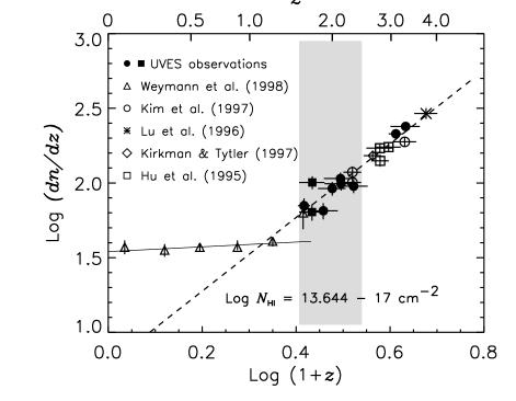
Figure 7: The number density evolution of the Ly$\alpha$ forest over the column density range $N_{\mathrm{H\,\mathsc{i}}}=10^{13.64-17}\ {\mathrm{cm}}^{-2}$, which is comparable to the HST data (open triangles) of Weymann et al. (1998). The data are shown for the binned sample for display. The filled symbols are derived from the UVES observations. Open squares, the star, open circles, and the diamond are taken from the HIRES data by Hu et al. (1995), Lu et al. (1996), Kim et al. (1997), and Kirkman & Tytler (1997), respectively. The horizontal error bars represent the $z$ interval over which the number density was estimated. The vertical error bars represent the Poisson $1\sigma$ error.

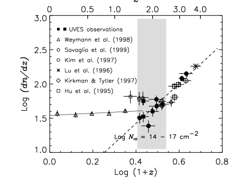
Figure 8: The number density evolution of the Ly$\alpha$ forest over the column density range $N_{\mathrm{H\,\mathsc{i}}}=10^{14-17}\ {\rm cm}^{-2}$. All the symbols have the same meaning as in Fig. 7.

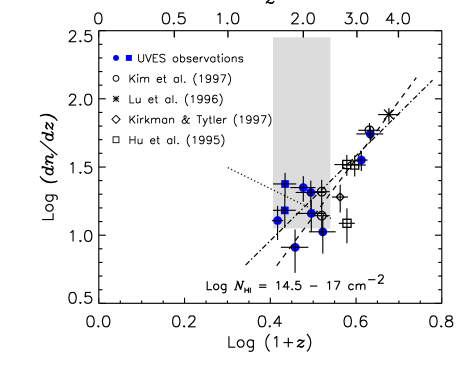
Figure 9: The number density evolution of the Ly$\alpha$ forest over the column density range $N_{\mathrm{H\,\mathsc{i}}}=10^{14.5-17}\ {\rm cm}^{-2}$. All the symbols have the same meaning as in Fig. 7. The dot-dashed line represents the single maximum likelihoold fit over the entire redshift ranges (see Table 3). The dotted line indicates the maximum likelihood fit for $z<2.5$: $dn/dz=91.3\,(1+z)^{-1.55\pm 1.49}$. The dashed line represents the maximum likelihood fit for $z>2.5$: $dn/dz=0.1\,(1+z)^{4.24\pm 0.88}$. The redshift 2.5 is chosen arbitrary.

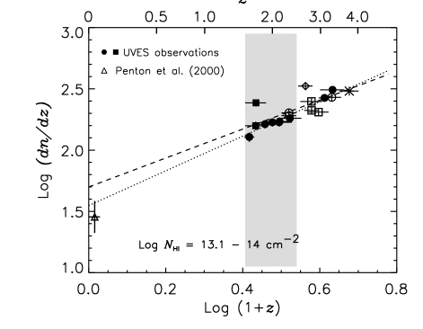
Figure 10: The number density evolution of the Ly$\alpha$ forest over the column density range $N_{\mathrm{H\,\mathsc{i}}}=10^{13.1-14}\ {\rm cm}^{-2}$. All the symbols unlisted in the figure are the same as in Fig. 7.

Figure 11: The value $\gamma$ as a function of the median $N_{\mathrm{H\,\mathsc{i}}}$ at the different column density ranges. The upper $N_{\mathrm{H\,\mathsc{i}}}$ threshold is fixed to be $N_{\mathrm{H\,\mathsc{i}}}=10^{17}\ {\rm cm}^{-2}$ (squares) and $N_{\mathrm{H\,\mathsc{i}}}=10^{16}\ {\rm cm}^{-2}$ (diamonds), respectively. The lower $N_{\mathrm{H\,\mathsc{i}}}$ threshold for each median $N_{\mathrm{H\,\mathsc{i}}}$, $N_{\rm{\mathrm{H\,\mathsc{i}}},med}=10^{13.3},\ 10^{13.6},\ 10^{13.9},\ 10^{14.3}$, and $10^{15.0}\ {\rm cm}^{-2}$, corresponds to be $N_{\mathrm{H\,\mathsc{i}}}=10^{12.5},\ 10^{13},\ 10^{13.5},\ 10^{14}$, and $10^{14.5}\ {\rm cm}^{-2}$, respectively.

3.2 The evolutionary behavior of $dn/dz$

As shown in Figs. 7–10, the break point in $dn/dz$ may occur at redshifts as low as $z\sim 1$, and very likely $z<1.5$, rather than $z\sim 1.7$–2 as suggested by Theuns et al. (1998) and Davé et al. (1999). This shows that the UV background does not decrease as rapidly as the QSO-dominated UV background by Haardt & Madau (1996) used in simulations, and so galaxies could be a main source of the UV background at $z<2.5$ and/or that the structure formation could be underestimated in simulations. Davé et al. (1999) show that $dn/dz\propto(1+z)^{5\beta-6.5}$ for a constant UV background in the flat Friedmann universe. For $N_{\mathrm{H\,\mathsc{i}}}=10^{13.64-17}\ {\mathrm{cm}}^{-2}$ at $1.5<z<4$, $\beta=1.74\pm 0.02$. This indicates $dn/dz\propto(1+z)^{2.25}$, which is in agreement with the observations, $dn/dz\propto(1+z)^{2.44\pm 0.18}$. This result suggests a non-decreasing UV background at $1.5<z<4$, unlike the decreasing one expected from the Haardt & Madau UV background at $z<2.5$, i.e. the QSOs alone might not be enough to explain the $dn/dz$ evolution of the forest (KCD; Bianchi et al. 2001).

Besides the break point in $dn/dz$ at $z\sim 1$, Lu et al. (1991) suggest that $dn/dz$ could be fit better with a double power-law at $z\sim 2.3$ for $1.6<z<3$, using the minimum $W$ threshold $W=0.36$Å. The minimum $W$ threshold corresponds to $N_{\mathrm{H\,\mathsc{i}}}=10^{14.7},\ 10^{14.4}$ and $10^{14.2}\ {\mathrm{cm}}^{-2}$ for $b=25$, 30 and 35 km s^-1, respectively. This threshold is similar to the one used in Fig. 9. As clearly seen in Fig. 9, there is no clear trend of a different evolution of $dn/dz$ at higher and lower redshifts.

The general trend shown in $dn/dz$ confirms that $dn/dz$ continues its evolution in the same general manner at least for $1.5<z<4$, which indicates the importance of the Hubble expansion over the structure formation at this redshift ranges (Miralda-Escudé et al. 1996; Theuns et al. 1998; Davé et al. 1999). Our new observations (Fig. 9), however, show that the structure evolution becomes more important in some lines of sights at $z<2.5$ and the clustering of stronger lines also increases as $z$ decreases (Fig. 17).

3.3 The mean H i opacity

As seen in Section 3.1, comparing the the line number densities at $z>1.5$ with those at $z<1.5$ is somewhat uncertain because of the different spectral resolutions used. The mean H i opacity provides more straightforward comparisons between different qualities of data. Moreover, the mean H i opacity does not rely on the subjective line counting method, although it is more subject to continuum uncertainties (KCD).

Fig. 12 shows the $\overline{\tau}_{\mathrm{H\,\mathsc{i}}}$ measurements (the effective optical depth $\tau_{\mathrm{eff}}$; $\exp^{-\tau_{\mathrm{eff}}}=\ <\!\exp^{-\tau}\!>$, where $<\,\,>$ indicates the mean value averaged over wavelength), together with other opacity measurements compiled from the literature. Filled symbols are the $\overline{\tau}_{\mathrm{H\,\mathsc{i}}}$ measurements from the UVES data. The dotted line represents a widely used $\tau_{\mathrm{eff}}$ from low-resolution data by Press, Rybicki & Schneider (1993). Table 2 lists the estimated $\overline{\tau}_{\mathrm{H\,\mathsc{i}}}$ values from the UVES observations (see KCD for the actual $\overline{\tau}_{\mathrm{H\,\mathsc{i}}}$ values at $z>1.5$ in Fig. 12, which is not listed in Table 2). Table 4 lists the estimated $\overline{\tau}_{\mathrm{H\,\mathsc{i}}}$ values from HST observations, adding the equivalent widths. The different $\overline{\tau}_{\mathrm{H\,\mathsc{i}}}$ values of 3C273 at the different $z$ ranges by different studies suggest the uncertainty in deriving $\overline{\tau}_{\mathrm{H\,\mathsc{i}}}$ as well as a small-scale cosmic variance.

The solid line represents the least-squares fit to the UVES (only filled circles and squares) and HIRES data: $\overline{\tau}_{\mathrm{H\,\mathsc{i}}}(z)=(0.0032\pm 0.0009)\,(1+z)^{3.37\pm 0.20}$. As stated in KCD, $\overline{\tau}_{\mathrm{H\,\mathsc{i}}}$ is well fit to a single power-law at $1.5<z<4$ and the newly fit power-law is about a factor of 1.3 smaller than the Press et al. value from their lower resolution data.

The square with higher $\overline{\tau}_{\mathrm{H\,\mathsc{i}}}$ at $z\sim 1.8$ is from HE2217–2818, which shows several high-$N_{\mathrm{H\,\mathsc{i}}}$ clouds at $N_{{\mathrm{H\,\mathsc{i}}}}=10^{14-17}{\mathrm{cm}}^{-2}$. This increases $\overline{\tau}_{\mathrm{H\,\mathsc{i}}}$ at $z\sim 1.8$, compared to that of HE1122–1648 without high-$N_{\mathrm{H\,\mathsc{i}}}$ clouds at the same redshift range. The bold open circle at $z\sim 2$ is $\overline{\tau}_{\mathrm{H\,\mathsc{i}}}$ towards J2233–606, when two higher column density absorption systems were excluded. Note that $\overline{\tau}_{\mathrm{H\,\mathsc{i}}}$ towards HE2217–2818 at $z\sim 1.8$ and J2233–606 are similar to the Press et al. value at the same redshifts. This confirms that the higher Press et al. value is in part due to the inclusion of high column density systems in their low resolution sample as well as the uncertainty in the continuum displacement, as noted by KCD. Keep in mind that most QSOs used in our analysis both from the UVES and Keck observations do show few high column density systems at $N_{{\mathrm{H\,\mathsc{i}}}}>10^{17}{\mathrm{cm}}^{-2}$. In the case of having a damped system along the sightline, such as Q1101–264 and Q0000–263, we excluded the regions in which the damped systems are located.

There is a large uncertainty in $\overline{\tau}_{\mathrm{H\,\mathsc{i}}}$ from HST observations due to their lower S/N, lower resolution, and lower absorption line densities with the presence of weak emission lines, all resulting in an unreliable local continuum fit. This, in general, leads to a tendency to miss weak lines and so an underestimate $\overline{\tau}_{\mathrm{H\,\mathsc{i}}}$. There is, however, indication of slow-down in the evolution of $\overline{\tau}_{\mathrm{H\,\mathsc{i}}}$. Despite a large scatter at $z\sim 0.1$, the median $\overline{\tau}_{\mathrm{H\,\mathsc{i}}}$ at $z\sim 0.1$ is 0.019, a factor of 4.3 larger than the value extrapolated from at $z>1.5$. Although open triangles (Weymann et al. 1998) might underestimate $\overline{\tau}_{\mathrm{H\,\mathsc{i}}}$ significantly, the different evolution in $\overline{\tau}_{\mathrm{H\,\mathsc{i}}}$ occurs at $z<1$, a bit lower than that suggested from $dn/dz$.

Davé et al. (1999) simulated the evolution of $\overline{\tau}_{\mathrm{H\,\mathsc{i}}}$, assuming different cosmologies and normalizing their results to observations at $z\sim 3$. The shaded area in Fig. 12 shows the ranges of $\overline{\tau}_{\mathrm{H\,\mathsc{i}}}$ from their simulations at $z<2$. Although the estimation of $\overline{\tau}_{\mathrm{H\,\mathsc{i}}}$ from HST observatons could be underestimated by a large factor, it is not in good agreement with the simulated $\overline{\tau}_{\mathrm{H\,\mathsc{i}}}$. In particular, at $z\sim 0.5$, there are some observations which show lower $\overline{\tau}_{\mathrm{H\,\mathsc{i}}}$ than the simulated one by more than a factor of 10. This could indicate that the QSO-dominated UV background by Haardt & Madau (1996) used in the simulations does not represent the real UV background at $z<2$, i.e. this Haardt & Madau QSO-dominated background underestimates the real UV background at $z<2$, as suggested by the evolution of $dn/dz$. In addition, the structure in the Ly$\alpha$ forest becomes more highly patchy at $z<2$ than the simulations predict (see Fig. 9). In the latter case, some lines of sight could have a very lower $\overline{\tau}_{\mathrm{H\,\mathsc{i}}}$.

Table 4: The mean H i opacity compiled from the literature

QSO	$z_{\mathrm{em}}$	$\Delta z$	$\overline{\tau}_{\mathrm{H\,\mathsc{i}}}$	Ref.
PKS0044+03	0.624	0.403–0.590	$0.024^{0.027}_{-0.021}$	1
3C95	0.614	0.394–0.580	$0.009^{0.009}_{-0.008}$	1
US1867	0.513	0.357–0.481	$0.005^{0.005}_{-0.004}$	1
3C263	0.652	0.357–0.617	$0.021^{0.024}_{-0.019}$	1
3C273	0.158	0.000–0.134	$0.010^{0.011}_{-0.009}$	1
PG1259+593	0.472	0.020–0.271	$0.008^{0.008}_{-0.007}$	1
PG1259+593	0.472	0.271–0.441	$0.008^{0.008}_{-0.007}$	1
3C351	0.371	0.069–0.342	$0.020^{0.021}_{-0.018}$	1
H1821+643	0.297	0.008–0.270	$0.022^{0.024}_{-0.020}$	1
PKS2145+06	0.990	0.481–0.719	$0.022^{0.024}_{-0.019}$	1
PKS2145+06	0.990	0.719–0.948	$0.034^{0.036}_{-0.031}$	1
3C454.3	0.859	0.398–0.606	$0.016^{0.019}_{-0.014}$	1
3C454.3	0.859	0.606–0.789	$0.012^{0.014}_{-0.010}$	1
PG1222+228a	2.046	0.892–1.262	$0.046^{0.057}_{-0.035}$	2
PG1222+228a	2.046	1.262–1.631	$0.073^{0.080}_{-0.067}$	2
PG1222+228a	2.046	1.631–1.715	$0.049^{0.055}_{-0.042}$	2
PG1634+706a	1.334	0.522–0.769	$0.040^{0.045}_{-0.035}$	2
PG1634+706a	1.334	0.769–1.016	$0.021^{0.023}_{-0.018}$	2
PG1634+706a	1.334	1.016–1.285	$0.027^{0.029}_{-0.024}$	2
PG2302+029a	1.044	0.892–1.001	$0.021^{0.025}_{-0.016}$	2
PG1211+143	0.085	0.006–0.062	$0.035^{0.038}_{-0.031}$	3
Q1214+1804	0.375	0.006–0.216	$0.039^{0.049}_{-0.029}$	3
PG1216+069	0.334	0.006–0.223	$0.025^{0.029}_{-0.022}$	3
PKS1217+023	0.240	0.006–0.214	$0.013^{0.015}_{-0.010}$	3
3C273	0.158	0.006–0.134	$0.008^{0.009}_{-0.006}$	3
J1230.8+0115	0.117	0.007–0.093	$0.019^{0.021}_{-0.017}$	3
Q1228+1116	0.235	0.007–0.209	$0.018^{0.023}_{-0.014}$	3
Q1230+0947	0.420	0.007–0.223	$0.013^{0.016}_{-0.011}$	3
Q1245–0333	0.379	0.007–0.223	$0.018^{0.022}_{-0.015}$	3
PKS1252+119	0.870	0.007–0.223	$0.016^{0.020}_{-0.012}$	3
Q1252+0200	0.345	0.007–0.223	$0.008^{0.010}_{-0.006}$	3
3C273	0.158	0.000–0.070	$0.021^{0.027}_{-0.016}$	4
H1821+643	0.297	0.013–0.042	$0.019^{0.026}_{-0.013}$	4
PKS2155–304	0.117	0.006–0.064	$0.046^{0.054}_{-0.038}$	4
Q1230+0115	0.117	0.001–0.032	$0.050^{0.064}_{-0.035}$	4

• The equivalent widths listed in the referenced paper are only for the core of the profile. Impey et al. (1996) gave a scale factor of 1.33 for isolated lines and of 1.18 for blended lines, to recover the total equivalent widths. We have used a scale factor of 1.255, a mean value.

• 1. Bahcall et al. (1993); 2. Impey et al. (1996); 3. Impey et al. (1999); 4. Penton et al. (2000).

Figure 12: The H i opacity as a function of $z$. Filled symbols represent the mean H i opacity from the UVES data. The open circle at $<\!z\!>\ =2.0$ represents $\overline{\tau}_{\mathrm{H\,\mathsc{i}}}$ of J2233–606 when two high column density systems are excluded. Other symbols at $z>1.5$ are from: open circles (Hu et al. 1995), large square (Lu et al. 1996), the open triangle (Kirkman & Tytler 1997), and diamonds (Rauch et al. 1997). Symbols at $z<1.5$ with arrows are from: open diamonds (Impey et al. 1996), open triangles (Weymann et al. 1998), open stars (Impey et al. 1999) and open squares (Penton et al. 2000). Due to the low resolution and low S/N spectra of the HST observations, ${\overline{\tau}}$ could be highly underestimated if the Ly$\alpha$ forest at $N_{\mathrm{H\,\mathsc{i}}}\leq 10^{14}\ {\mathrm{cm}}^{-2}$ contains the bulk of the neutral hydrogen. $\overline{\tau}_{\mathrm{H\,\mathsc{i}}}$ estimates, while the y-axis error bars were estimated from simply changing the adopted continuum by $\pm 5$%. The dotted line represents the commonly used formula by Press et al. (1993), ${\overline{\tau}}_{\mathrm{{\mathrm{H\,\mathsc{i}}}}}(z)=0.0037\,(1+z)^{3.46}$. The shaded area enclosed with dot-dashed lines indicates the ranges of ${\overline{\tau}}$ expected from different cosmological simulations by Davé et al. (1999).

3.4 The differential density distribution function

The differential density distribution function, $f(N_{\mathrm{H\,\mathsc{i}}})$, is defined as the number of the absorption lines per unit absorption distance path and per unit column density as a function of $N_{\mathrm{H\,\mathsc{i}}}$. The absorption distance path $X(z)$ is defined by $X(z)\equiv{1\over 2}[(1+z)^{2}-1]$ for $q_{\mathrm{o}}=0$ or by $X(z)\equiv{2\over 3}[(1+z)^{3/2}-1]$ for $q_{\mathrm{o}}=0.5$ in the standard Friedmann universe (see Table 2 for $q_{\mathrm{o}}=0$). Empirically, $f(N_{\mathrm{H\,\mathsc{i}}})$ is fitted to a power law: $f(N_{\mathrm{H\,\mathsc{i}}})=A\,N_{\mathrm{H\,\mathsc{i}}}^{-\beta}$.

Fig. 13 shows the observed $f(N_{\mathrm{H\,\mathsc{i}}})$ at different redshift ranges without the incompleteness correction due to line blending. The dotted line represents the incompleteness-corrected $f(N_{\mathrm{H\,\mathsc{i}}})$ at $<\!z\!>\ =2.85$ from Hu et al. (1995), $f(N_{\mathrm{H\,\mathsc{i}}})=4.9\times 10^{7}\,N_{\mathrm{H\,\mathsc{i}}}^{-1.46}$. Triangles for the damped Ly$\alpha$ systems at $1.5<z<2.5$ are taken from Storrie-Lombardi & Wolfe (2000). At $z\sim 2.1$, $f(N_{\mathrm{H\,\mathsc{i}}})$ at $N_{\mathrm{H\,\mathsc{i}}}=10^{12.5-14.5}\ {\mathrm{cm}}^{-2}$ is in good agreement with the incompleteness-corrected $f(N_{\mathrm{H\,\mathsc{i}}})$ at $z\sim 2.8$. It is also true for $f(N_{\mathrm{H\,\mathsc{i}}})$ at $z\sim 3.3$, although the goodness-of-the-fit is lower at $N_{\mathrm{H\,\mathsc{i}}}=10^{12.5-13}\ {\mathrm{cm}}^{-2}$. In general, $f(N_{\mathrm{H\,\mathsc{i}}})$ is well approximated to a single power-law $f(N_{\mathrm{H\,\mathsc{i}}})\propto N_{\mathrm{H\,\mathsc{i}}}^{-1.5}$ at $N_{\mathrm{H\,\mathsc{i}}}=10^{12.5-22}\ {\mathrm{cm}}^{-2}$ (Petitjean et al. 1993).

As noted by Petitjean et al. (1993) and Kim et al. (1997), $f(N_{\mathrm{H\,\mathsc{i}}})$ starts to deviate from the empirical power-law at $N_{\mathrm{H\,\mathsc{i}}}>10^{14}\ {\mathrm{cm}}^{-2}$. The amount of this deviation increases as $z$ decreases since the higher $N_{\mathrm{H\,\mathsc{i}}}$ forest disappears more rapidly as $z$ decreases. In addition, the deviation $N_{\mathrm{H\,\mathsc{i}}}$ at which $f(N_{\mathrm{H\,\mathsc{i}}})$ starts to deviate decreases as $z$ decreases. At $<\!z\!>\ =$ 3.8, 3.3 and 2.1, $f(N_{\mathrm{H\,\mathsc{i}}})$ deviates from the power-law at $N_{\mathrm{H\,\mathsc{i}}}\sim 10^{16}\ {\mathrm{cm}}^{-2}$, $N_{\mathrm{H\,\mathsc{i}}}\sim 10^{14.5}\ {\mathrm{cm}}^{-2}$ and $N_{\mathrm{H\,\mathsc{i}}}\sim 10^{14.2}\ {\mathrm{cm}}^{-2}$, respectively. At $N_{\mathrm{H\,\mathsc{i}}}>10^{15.6}\ {\mathrm{cm}}^{-2}$, the deviation from the single power-law increases more than $3\sigma$ at $z\sim 2.1$ and more than $2\sigma$ at $z\sim 3.3$. Table 5 lists $\log A$ and $\beta$ for the various column density ranges from the maximum-likelihood fit.

Figure 13: The differential density distribution functions at $<\!z\!>\,=2.1$, 3.3 and 3.8, without the incompleteness correction. The data are shown in the binned sample for display. Open triangles are the differential density distribution functions for the damped Ly$\alpha$ systems at $1.5<z<2.5$ (Storrie-Lombardi & Wolfe 2000). The dotted line represents the incompleteness-corrected $f(N_{\mathrm{H\,\mathsc{i}}})$ at $<\!z\!>\ =2.85$ from Hu et al. (1995), $f(N_{\mathrm{H\,\mathsc{i}}})=4.9\times 10^{7}\,N_{\mathrm{H\,\mathsc{i}}}^{-1.46}$.

Figure 14: The slope $\beta$ as a function of the $N_{\mathrm{H\,\mathsc{i}}}$ range used in the maximum likelihood fit.

Fig. 14 shows $\beta$ as a function of the $N_{\mathrm{H\,\mathsc{i}}}$ range. The x-axis error bars represent the $N_{\mathrm{H\,\mathsc{i}}}$ range used in the fit. For $N_{\mathrm{H\,\mathsc{i}}}<10^{14.5}\ {\mathrm{cm}}^{-2}$, $\beta$ increases as $N_{\mathrm{H\,\mathsc{i}}}$ increases, in part due to incompleteness at $N_{\mathrm{H\,\mathsc{i}}}\leq 10^{13}\ {\mathrm{cm}}^{-2}$ (Hu et al. 1995; Giallongo et al. 1996, see also Section 3.1). For $N_{\mathrm{H\,\mathsc{i}}}>10^{14.5}\ {\mathrm{cm}}^{-2}$, $\beta$ is ill-defined since there are not enough lines in the samples to get a reliable $\beta$, especially at $z\sim 2.1$.

Although it is statistically uncertain, there is a suggestion of increasing $\beta$ as $z$ decreases for a given $N_{\mathrm{H\,\mathsc{i}}}$ range in Fig. 14. Even if we exclude the lower-$N_{\mathrm{H\,\mathsc{i}}}$ range distorted by line blending, the similar trends hold. Table 5 lists the $\beta$ values at $<\!z\!>\ =0.03$ using the conversion from $W$ by Penton et al. (2000) and the $\beta$ value at $<\!z\!>\ =0.17$ using the direct profile fitting analysis by Davé & Tripp (2001) for different column density ranges. Even if we discard the $\beta$ values by Penton et al. (2000) due to their $W$ analysis, the $\beta$ value at $<\!z\!>\ =0.17$ suggests that $\beta$ increases as $z$ decreases. This is another way of showing that the strong Ly$\alpha$ forest evolves rapidly at $0<z<4$.

3.5 The differential mass density distribution of the Ly$\alpha$ forest

Schaye (2001) has shown that the shape of the differential density distribution function reflects that of the differential mass density distribution function as a function of the gas density. This differential mass density distribution function of the Ly$\alpha$ forest is the mass density per unit overdensity $\delta$. Assuming that the gas is isothermal, it can be described by

$$\frac{d\Omega_{\mathrm{g}}}{d\log(1+\delta)}\sim 7.6\times 10^{-9}\,h^{-1}\,\Gamma_{12}^{1/3}\,T_{4}^{0.59}\,$$

$$\\ \times{\left(\frac{f_{\mathrm{g}}}{0.16}\right)}^{1/3}\,N_{\mathrm{H\,\mathsc{i}}}^{4/3}\,f(N_{\mathrm{H\,\mathsc{i}}},z),$$ (1)

where $N_{\mathrm{H\,\mathsc{i}}}$ is related to $\delta$ through

$$N_{\mathrm{H\,\mathsc{i}}}\sim 2.7\times 10^{13}(1+\delta)^{1.5}\,T_{4}^{-0.26}\Gamma^{-1}_{12}$$

$$\\ \times{\left(\frac{1+z}{4}\right)}^{9/2}\,{\left(\frac{\Omega_{\mathrm{b}}\,h^{2}}{0.02}\right)}^{3/2}\,{\left(\frac{f_{\mathrm{g}}}{0.16}\right)}^{1/3}$$ (2)

(Schaye 2001). The parameter $h$ is the Hubble constant divided by 100, the H i photoionization rate $\Gamma\equiv\Gamma_{12}\times 10^{12}$ s^-1, the temperature of the Ly$\alpha$ forest $T\equiv T_{4}\times 10^{4}$ K, $f(N_{\mathrm{H\,\mathsc{i}}},z)$ is the differential density distribution function as a function of $z$, $f_{\mathrm{g}}$ is a fraction of mass in the Ly$\alpha$ forest and $\Omega_{\mathrm{b}}$ is the baryon density (Schaye 2001). As the gas is assumed to be isothermal in Eq. 1, $T$ is assumed to be constant ($\alpha=0$ in $T\propto(1+\delta)^{\alpha}$), i.e. not a function of $(1+\delta)$. The $d\Omega_{\mathrm{g}}/d\log(1+\delta)$ values, however, do not vary much with $\alpha$.

If $f(N_{\mathrm{H\,\mathsc{i}}},z)\propto N_{\mathrm{H\,\mathsc{i}}}^{-\beta}$, $\Omega_{\mathrm{g}}\propto\int N_{\mathrm{H\,\mathsc{i}}}^{4/3-\beta}\,d\ln N_{\mathrm{H\,\mathsc{i}}}$ (Schaye 2001). If the differential density distribution function is a single power-law, then $d\Omega_{\mathrm{g}}/d\log(1+\delta)\propto N_{\mathrm{H\,\mathsc{i}}}^{4/3-\beta}$. Therefore, the shape of $d\Omega_{\mathrm{g}}/d\log(1+\delta)$ reflects the deviation from the single power-law of $f(N_{\mathrm{H\,\mathsc{i}}},z)$. As seen in Fig. 14, $\beta$ is not a constant. If $\beta<4/3$, $d\Omega_{\mathrm{g}}/d\log(1+\delta)$ increases. Therefore, $d\Omega_{\mathrm{g}}/d\log(1+\delta)$ is expected to increase at smaller $N_{\mathrm{H\,\mathsc{i}}}$ and to decrease at larger $N_{\mathrm{H\,\mathsc{i}}}$.

Fig. 15 shows the differential mass density distribution function $d\Omega_{\mathrm{g}}/d\log(1+\delta)$ as a function of $N_{\mathrm{H\,\mathsc{i}}}$ at three redshifts. The arrow in Fig. 15 indicates the direction towards which $d\Omega_{\mathrm{g}}/d\log(1+\delta)$ moves if $T_{4}$ or $\Gamma_{12}$ increase, i.e. preserves the shape of $d\Omega_{\mathrm{g}}/d\log(1+\delta)$. The QSO-dominated UV background by Haardt & Madau (1996), $J_{\mathrm{HM}}$, was assumed in the Friedmann universe with $h=0.65$. Other parameters are obtained from the observations, while $T_{4}$ was read from figure 3 by Schaye et al. (2000).

There is a turnover at $N_{\mathrm{H\,\mathsc{i}}}\sim 10^{13}\ {\mathrm{cm}^{-2}}$ due to line blending as seen in Fig. 13 and in part due to the real deficiency of these weaker lines (cf. Schaye 2001). The amount of the turnover is more significant at $z\sim 3.8$ and the turnover occurs at lower $N_{\mathrm{H\,\mathsc{i}}}$ at lower $z$. At $N_{\mathrm{H\,\mathsc{i}}}\approx 10^{13.5-15}\ {\mathrm{cm}^{-2}}$, $d\Omega_{\mathrm{g}}/d\log(1+\delta)$ is roughly approximated by a single power-law, with a slope being slightly steeper at lower $z$. This indicates that $\beta$ is larger at lower $z$ and that $\beta$ at all $z$ is larger than $4/3$. At $N_{\mathrm{H\,\mathsc{i}}}>10^{15}\ {\mathrm{cm}^{-2}}$, $d\Omega_{\mathrm{g}}/d\log(1+\delta)$ is not clearly defined due to a larger size of the $N_{\mathrm{H\,\mathsc{i}}}$ bin (also due to a smaller number of lines at this column density regime).

The three curves for $d\Omega_{\mathrm{g}}/d\log(1+\delta)$ at different redshifts agree with each other reasonably well with each other if one applies a redshift-dependent offset in $N_{\mathrm{H\,\mathsc{i}}}$, at least in the range $N_{\mathrm{H\,\mathsc{i}}}\approx 10^{13-15}\ {\mathrm{cm}^{-2}}$ (referenced to $<z>=3.3$). In fact, $d\Omega_{\mathrm{g}}/d\log(1+\delta)$ as a function of $(1+\delta)$ does show a similar shape at different $z$. Eq. 2 shows that any change in $z$ and $\Gamma_{12}$ (thus $T_{4}$) reflects the relation between $N_{\mathrm{H\,\mathsc{i}}}$ and $(1+\delta)$. Thus, Fig. 15 indicates that the redshift-evolution of the differential density distribution function seen at $N_{\mathrm{H\,\mathsc{i}}}=10^{13-15}\ {\mathrm{cm}^{-2}}$ reflects the change in $\Gamma$ at different $z$ (Schaye 2001).

Figure 15: The differential mass density distribution of the Ly$\alpha$ forest as a function of $N_{\mathrm{H\,\mathsc{i}}}$. Among the parameters used in Eq. 1 and Eq. 2, $\Gamma_{12}$ was read from figure 8 of Haardt & Madau (1996) and $T_{4}$ was read from figure 3 of Schaye et al. (2000) for their simulations under $J_{\mathrm{HM}}$ at $\delta=1$. The parameters $f_{\mathrm{g}}$, $\Omega_{\mathrm{b}}\,h^{2}$ and $h$ are assumed to be 0.16, 0.02 and 0.65, respectively, in the flat Friedmann universe. At $<\!z\!>\ =2.1$, 3.3 and 3.8, $(T_{4},\Gamma_{12})$ is $(1.41,1.35)$, $(1.57,1.07)$ and $(1.62,0.7)$, respectively. The arrow indicates the direction towards which $d\Omega_{\mathrm{g}}/d\log(1+\delta)$ moves if $T_{4}$ or $\Gamma_{12}$ increases.

Table 5: The power-law fit of the distribution functions, $f(N_{\mathrm{H\,\mathsc{i}}})=A\,N_{\mathrm{H\,\mathsc{i}}}^{-\beta}$

	$N_{\mathrm{H\,\mathsc{i}}}=10^{12.5-14}\ \mathrm{cm}^{-2}$			$N_{\mathrm{H\,\mathsc{i}}}=10^{14-16}\ \mathrm{cm}^{-2}$			$N_{\mathrm{H\,\mathsc{i}}}=10^{13-17}\ \mathrm{cm}^{-2}$			$N_{\mathrm{H\,\mathsc{i}}}=10^{14.5-17}\ \mathrm{cm}^{-2}$
$<\!z\!>$	$\log A$	$\beta$		$\log A$	$\beta$		$\log A$	$\beta$		$\log A$	$\beta$
0.03a	$11.3\pm 0.7$	$1.72\pm 0.06$		$7.4\pm 5.2$	$1.43\pm 0.35$		-	-		-	-
0.17b	-	-		-	-		$10.87\pm 0.12$	$2.04\pm 0.23$		-	-
2.1	$7.11\pm 1.49$	$1.42\pm 0.03$		$12.82\pm 1.01$	$1.87\pm 0.11$		$11.00\pm 1.38$	$1.71\pm 0.03$		$10.11\pm 0.79$	$1.66\pm 0.14$
3.3	$3.26\pm 1.33$	$1.11\pm 0.04$		$12.21\pm 1.04$	$1.75\pm 0.09$		$9.18\pm 1.31$	$1.55\pm 0.03$		$11.40\pm 0.82$	$1.70\pm 0.13$
3.8	$1.94\pm 1.17$	$1.01\pm 0.01$		$10.56\pm 0.98$	$1.63\pm 0.09$		$7.77\pm 1.22$	$1.44\pm 0.03$		$7.15\pm 0.81$	$1.41\pm 0.11$

• Penton et al. (2000).

• Davé & Tripp (2001).

3.6 The two-point function of the flux

The line width of the absorption lines (the $b$ parameter from the Voigt profile fitting) provides valuable information on the thermal temperature of the absorption clouds, if the Ly$\alpha$ forest is thermally broadened. In particular, the lower envelope of the $N_{\mathrm{H\,\mathsc{i}}}$–$b$ diagram is interpreted to give an upper limit on the temperature (through $b$) of the forest as a function of $N_{\mathrm{H\,\mathsc{i}}}$ (Schaye et al. 1999; McDonald et al. 2000; Ricotti, Gnedin & Shull 2000; Schaye et al. 2000; KCD; Kim, Cristiani & D’Odorico 2002). However, it is not straightforward to determine this minimum $b$ value as a function of $N_{\mathrm{H\,\mathsc{i}}}$, particularly because of profile fitting errors in blended features.

Instead of using the fitted parameters, the direct use of normalized flux, $F$, has been proposed (Miralda-Escudé et al. 1997; Bryan et al. 1999; Machacek et al. 2000; Theuns et al. 2000). Among these flux-based properties of the Ly$\alpha$ forest, the two-point function of the flux provides the profile shape of absorption lines at $30<\Delta v<100$ km s^-1 (Machacek et al. 2000; Theuns et al. 2000).

The two-point function of the flux, $P(F_{1},F_{2},\Delta v)$, is the probability of two pixels with the $\Delta v$ velocity separation having normalized fluxes $F_{1}$ and $F_{2}$. It is described as

$$\overline{\Delta F}(\Delta v,\delta F_{1})$$

$$\equiv\int_{\delta F_{1}}\,\left[\int^{\infty}_{-\infty}(F_{1}-F_{2})P(F_{1},F_{2},\Delta v)\,dF_{2}\right]\,dF_{1}/\delta F_{1},$$ (3)

where $\overline{\Delta F}(\Delta v,\delta F_{1})$ is the mean flux difference between two pixels with $F_{1}$ and $F_{2}$, which are separated by $\Delta v$ (Theuns et al. 2000).

Fig. 16 shows $\overline{\Delta F}$ for $0.05<F<0.15$ at different redshifts. We measured the $\Delta v(0.3)$ value, following the definition by Machacek et al. (2000), the width of $\overline{\Delta F}(\Delta v,\delta F_{1})$ at which $\overline{\Delta F}(\Delta v,\delta F_{1})$ becomes 0.3. The individual QSOs show a different $\Delta v(0.3)$ even at the same $z$. The measured $\Delta v(0.3)$ averaged at each $z$ is 30.2 km s^-1, 33.7 km s^-1 and 48.8 km s^-1 at $<\!z\!>\ =$ 2.1, 3.3 and 3.8, respectively. This result might indicate that the line profile becomes broader as $z$ increases. In fact, Theuns et al. (2000) note that at a given $z$ a simulation with a hotter gas temperature shows a wider $\overline{\Delta F}(\Delta v,\delta F_{1})$ profile than a simulation with a lower gas temperature.

Decreasing $\Delta v(0.3)$ as decreasing $z$, however, is not an indicative of decreasing in temperature. The reason of decreasing $\Delta v(0.3)$ is that $\overline{\Delta F}(\Delta v,\delta F_{1})$ must be asymptotic to $\overline{F}-0.1$ and $\overline{F}$ decreases as $z$ increases (Theuns et al. 2000). Since $\overline{F}$ depends on $z$, comparing $\Delta v(0.3)$ at different $z$ directly does not provide any information on the temperature.

There is another way to look at decreasing $\Delta v(0.3)$ with decreasing $z$. From the minimum cutoff $b$ distribution at each $z$ from the same data, Kim et al. (2002) show that the minimum cutoff $b$ values increase as $z$ decreases (cf. Kim et al. 1997). This result shows that the $b$ (i.e. line width) values of absorption lines increases as $z$ decreases. This result is contrary to the result from $\overline{\Delta F}(\Delta v,\delta F_{1})$. This analysis of the minimum cutoff $b$ values suggests that $\overline{\Delta F}(\Delta v,\delta F_{1})$ actually measures the relative amounts of line blending and higher-$N_{\mathrm{H\,\mathsc{i}}}$ forest, when it is compared at different redshifts. The $\Delta v(0.3)$ values increase as $z$ increases due to more severe blending and more higher-$N_{\mathrm{H\,\mathsc{i}}}$ forest at higher $z$, not due to increasing temperature of absorbing clouds. $\overline{\Delta F}(\Delta v,\delta F_{1})$ for higher $F$ ranges, i.e. excluding higher column density lines, does not show any $z$-dependence.

Figure 16: The $\overline{\Delta F}(\Delta v,\delta F_{1})$ profile for $0.05<F<0.15$ at different redshifts. The left panel is for individual QSOs of Sample A, while the right panel is averaged for each $z$ bin.

3.7 The optical depth correlation function

We analysed the clustering properties of the Ly$\alpha$ forest, using the step optical depth correlation function (Cen et al. 1998; KCD). The optical depth correlation function is less biased than the line correlation functions since the fitted lines from Voigt profile fitting are not unique.

The step optical depth correlation function $\xi_{\tau,{\rm s}}$ is defined by

$$\xi_{\tau,{\rm s}}(\Delta v)\equiv\frac{<\tau_{\rm s}(v+\Delta v)\tau_{\rm s}(v)>}{<\tau_{\rm s}>^{2}}-1,$$ (4)

where the step optical depth, $\tau_{\mathrm{s}}$, is $\tau_{\mathrm{s}}=0$ if $\tau_{\mathrm{obs}}\leq\tau_{\mathrm{min}}$ and $\tau_{\mathrm{s}}=1$ if $\tau_{\mathrm{obs}}\geq\tau_{\mathrm{min}}$.

Fig. 17 shows $\xi_{\tau,{\rm s}}(\Delta v)$ averaged at each $z$ for $\tau_{\mathrm{min}}=2$. The $\tau_{\mathrm{min}}=2$ corresponds to $N_{\mathrm{H\,\mathsc{i}}}\sim 10^{13.6}\ {\mathrm{cm}}^{-2}$, if $b$ is assumed to be $b=30$ km s^-1. Dotted lines, dashed lines and the dot-dashed line represent the individual QSOs in each $z$ bin at $<\!z\!>\ =$ 2.1, 3.3 and 3.8. The large error bars at $<\!z\!>\ =2.1$ are due to the fact that the correlation strengths of different QSOs at similar redshifts show a wide range. Although there is a large scatter at $<\!z\!>\ =$ 2.1, the step optical depth correlation functions show a strong clustering at $v<100$ km s^-1. In addition, the step optical depth correlation strength increases as $z$ decreases in general. At $<\!z\!>\ =2.1$, $\xi_{\tau,{\rm s}}$ (50 km s^-1) shows a $\sim 10\sigma$ significance compared to that at $<\!z\!>\ =3.3$. This stronger clustering of the Ly$\alpha$ forest at $z\leq 2$ compared to higher $z$ is expected from the differences in $dn/dz$ and $\overline{\tau}_{\mathrm{H\,\mathsc{i}}}$ along the different sightlines. Studies of the two-point velocity correlation strength using the fitted line parameters at $z<1.5$ and $z>2.5$ also show a velocity correlation at $\Delta v\approx$ 50–500 km s^-1, although its significance is much smaller than that of the step optical depth correlation function (Ulmer 1996; Cristiani et al. 1997; Penton et al. 2000).

Figure 17: The step optical depth correlation functions at $<\!z\!>\ =2.1$ (squares), $<\!z\!>\ =3.3$ (diamonds) and $<\!z\!>\ =3.8$ (triangles). Error bars are the $1\sigma$ statistical errors from the sample size.

4 The Ly$\beta$ forest

At $N_{\mathrm{H\,\mathsc{i}}}\geq 10^{14}\ {\mathrm{cm}^{-2}}$, the Ly$\alpha$ forest absorption lines start to saturate. For single lines, this saturation results in an increasingly inaccurate estimation of $N_{\mathrm{H\,\mathsc{i}}}$ and $b$ as the ${\mathrm{H\,\mathsc{i}}}$ column density increases, at least up to the stage where damping wings become significant. More importantly, saturation also results in the uncertainty in the number of subcomponents present. In reality, some high-$N_{\mathrm{H\,\mathsc{i}}}$ clouds are not a really high-$N_{\mathrm{H\,\mathsc{i}}}$ cloud, but a blend of several lower-$N_{\mathrm{H\,\mathsc{i}}}$ clouds. Many of these saturated lines could have more accurate measurements of $N_{\mathrm{H\,\mathsc{i}}}$, $b$ and a number of subcomponents if the higher order Lyman lines are fitted simultaneously with the Ly$\alpha$, since the oscillator strengths decrease monotonically as one goes up the Lyman series.

Fitting the absorption profiles with higher-order series becomes more time-consuming as $z$ increases. In some cases, severe contamination by lower-$z$ Ly$\alpha$ forest and by the other higher-order Lyman series from higher-$z$ forest make it very difficult to deblend the saturated Ly$\alpha$ lines properly. In addition, S/N of $\geq 15$–20 is required to determine the continuum with adequate reliability. For these reasons, we have only fitted two QSO spectra with S/N $\sim$ 10–30 in the Ly$\beta$ regions, HE1122–1648 and HE2217–2818.

4.1 The line number density evolution of the Ly$\beta$ forest

Fig. 18 shows the line number density, $dn/dz$, of the Ly$\beta$ forest (filled symbols) and the Ly$\alpha$ forest both from Sample A and Sample B (open symbols). For $N_{\mathrm{H\,\mathsc{i}}}=10^{14-17}\ {\mathrm{cm}}^{-2}$, $dn/dz$ of the Ly$\beta$ forest is within the error bars of $dn/dz$ of the Ly$\alpha$ forest. In the case of HE2217–2818, $dn/dz$ of the Ly$\beta$ forest is less than $1\sigma$ different from that of the Ly$\alpha$ forest (14 versus 15 lines). For HE1122–1648, it becomes 27 versus 25 lines, well within the error bars. On the other hand, for $N_{\mathrm{H\,\mathsc{i}}}=10^{13.1-14}\ {\mathrm{cm}}^{-2}$, $dn/dz$ of the Ly$\beta$ forest systems shows a larger deviation. For HE2217–2818 (for HE1122–1648), it is 74 versus 68 lines (77 versus 62 lines). The main reasons for this difference in $dn/dz$ come in part from the continuum re-adjustment in the Ly$\alpha$-Ly$\beta$ fit (which has a more significant effect on the lower $N_{\mathrm{H\,\mathsc{i}}}$ forest) and in part from the more correct deblending of the higher-$N_{\mathrm{H\,\mathsc{i}}}$ forest. When the higher-$N_{\mathrm{H\,\mathsc{i}}}$ forest is deblended into more components, the number of lower-$N_{\mathrm{H\,\mathsc{i}}}$ components in the forest increases. This results in the higher number of smaller $N_{\mathrm{H\,\mathsc{i}}}$ forest from using the line parameters determined from fitting the Ly$\alpha$-Ly$\beta$ forest.

In general, however, the uncertainty in $dn/dz$ of the Ly$\beta$ forest is in the same amount or less than the uncertainty resulted from the different sightlines, i.e. the cosmic variance. The determination of $dn/dz$ from the Ly$\alpha$ forest alone does not affect the overall results of $dn/dz$ at least at $1.5<z<2.5$. At higher $z$, more severe line blending is likely to produce higher uncertainties in the reliable number of subcomponents in the saturated lines. This might result in a significantly different $dn/dz$ of the Ly$\beta$ forest at $z>3$, i.e. a higher $dn/dz$, compared to that of the Ly$\alpha$ forest.

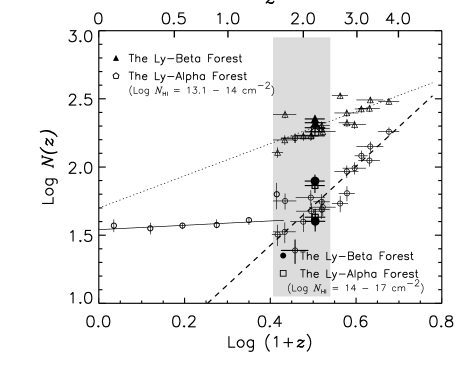
Figure 18: The line number density evolution of the Ly$\alpha$ forest and the Ly$\beta$ forest. Open circles represent all the different symbols from Fig. 8, while open triangles are from Fig. 10. The dashed line and the dotted line represent the maximum-likelihood fit of the Ly$\alpha$ forest for each $N_{\mathrm{H\,\mathsc{i}}}$ range in the fit.

4.2 The differential density distribution function of the Ly$\beta$ forest

Fig. 19 shows the differential column density distribution function, $f(N_{\mathrm{H\,\mathsc{i}}})$, for the Ly$\alpha$-only fit (open squares) and for the Ly$\alpha$-Ly$\beta$ fit (filled circles). At $N_{\mathrm{H\,\mathsc{i}}}\leq 10^{14.3}\ {\mathrm{cm}}^{-2}$, there is no significant difference in the Ly$\beta$ forest and the Ly$\alpha$ forest. The Kolmogorov-Smirnov test gives the KS statistic of 0.06 and the probability of 0.56. Note that a slight difference in $f(N_{\mathrm{H\,\mathsc{i}}})$ is due to the continuum fitting adjustment when the Ly$\alpha$ and the Ly$\beta$ forest lines were fitted simultaneously.

The difference seems to become more noticeable at $N_{\mathrm{H\,\mathsc{i}}}\geq 10^{14.3}\ \mathrm{cm}^{-2}$. This is, however, in part caused by the fact that there are not many high-$N_{\mathrm{H\,\mathsc{i}}}$ clouds in the sample (22 lines in the Ly$\beta$ forest sample and 18 lines in the Ly$\alpha$ forest sample) and in part by the fact that Fig. 19 shows the binned data for the display purpose. In fact, the Kolmogorov-Smirnov test gives the KS statistic of 0.22 and the probability of 0.65. Although it is a statistically small sample, Table 6 lists $f(N_{\mathrm{H\,\mathsc{i}}})$ at different $N_{\mathrm{H\,\mathsc{i}}}$ ranges. Within the error bars, $f(N_{\mathrm{H\,\mathsc{i}}})$ from both the Ly$\alpha$ forest and the Ly$\beta$ forest is in good agreement.

Table 6: The power-law fit of the distribution functions, $f(N_{\mathrm{H\,\mathsc{i}}})=A\,N_{\mathrm{H\,\mathsc{i}}}^{-\beta}$ at $<\!z\!>\ =2.2$

	$N_{\mathrm{H\,\mathsc{i}}}=10^{12.5-14.3}\ \mathrm{cm}^{-2}$			$N_{\mathrm{H\,\mathsc{i}}}=10^{14.3-17}\ \mathrm{cm}^{-2}$
	$\log A$	$\beta$		$\log A$	$\beta$
Ly$\alpha$	$7.40\pm 1.31$	$1.43\pm 0.04$		$11.57\pm 0.69$	$1.74\pm 0.17$
Ly$\beta$	$7.52\pm 1.34$	$1.43\pm 0.04$		$11.92\pm 0.75$	$1.76\pm 0.15$

4.3 The distribution of the Doppler parameters of the Ly$\beta$ forest

One of the important physical properties of the Ly$\alpha$ forest, the temperature of the absorbing gas, can be derived from the distribution of the Doppler ($b$) parameters. At higher $z$, the absorption lines are broadened by the thermal motion as well as the bulk motions. Therefore, the lower cutoff envelope of the $N_{\mathrm{H\,\mathsc{i}}}$–$b$ distribution constrains an upper limit on the thermal temperature of the forest as a function of $N_{\mathrm{H\,\mathsc{i}}}$ at a given $z$ (Hui & Gnedin 1997; Schaye et al. 1999; McDonald et al. 2000; Ricotti et al. 2000; KCD; Davé & Tripp 2001; Kim et al. 2002).

Fig. 20 shows the distribution of the Doppler parameters of the Ly$\alpha$ (dashed lines) and the Ly$\beta$ forest (solid lines). For $N_{\mathrm{H\,\mathsc{i}}}=10^{12.5-14.5}\ {\mathrm{cm}}^{-2}$ (the left hand panel), the median $b$ is 27.6 km s^-1 (the Ly$\beta$ forest) and 26.84 km s^-1 (the Ly$\alpha$ forest). There is no significant difference in the $b$ distribution between the Ly$\alpha$ forest and the Ly$\beta$ forest for this $N_{\mathrm{H\,\mathsc{i}}}$ range. This result confirms the validity of the determination of the lower cutoff $b$ values using the Ly$\alpha$ forest in previous studies since the lower cutoff has been derived at $N_{\mathrm{H\,\mathsc{i}}}=10^{12.5-14.5}\ {\mathrm{cm}}^{-2}$. Since these lines are not saturated, lower cutoff $b$ values from the Ly$\alpha$ forest would not be changed, when the Ly$\alpha$ forest is fit simultaneously with the Ly$\beta$ forest. In fact, the $N_{\mathrm{H\,\mathsc{i}}}$–$b$ diagram from the Ly$\alpha$ forest and the Ly$\beta$ forest does not show any significant difference.

The right hand panel of Fig. 20 shows the $b$ distributions for $N_{\mathrm{H\,\mathsc{i}}}=10^{14.5-17}\ {\mathrm{cm}}^{-2}$. The median $b$ is 34.0 km s^-1 (the Ly$\beta$ forest; 15 lines) and 32.7 km s^-1 (the Ly$\alpha$ forest; 13 lines). Although the median values are not statistically robust due to the small number of available lines, there is no significant difference between the Ly$\alpha$ and the Ly$\beta$ forest for this higher $N_{\mathrm{H\,\mathsc{i}}}$ range, either.

Table 7 lists the observed $\overline{b}$ values and the median $b$ values from the Ly$\beta$ forest as well as the ones at $z\sim 0.15$. Our characteristic $b$-values at $z\sim 2.2$ are very similar to those reported by Shull et al. (2000) from the curve-of-growth analysis. On the other hand, our values are somewhat larger than those of Davé & Tripp (2001) obtained from a profile fitting analysis. Table 7 shows that there is no significant difference of $\overline{b}$ and median $b$ values between the Ly$\alpha$ forest and the Ly$\beta$ forest at $z\sim 2.2$. Although $\overline{b}$ and median $b$ values are dependent on $N_{\mathrm{H\,\mathsc{i}}}$ ranges, Table 8 suggests that the median $b$ value does not increase, i.e. constant or decreasing, at $z<1.5$ from at $z\sim 2.1$ for two $N_{\mathrm{H\,\mathsc{i}}}$ ranges considered in Table 8 (see KCD; Kim et al. 2002).

Table 7: The characteristic $b$ values of the Ly$\beta$ forest

$<\!z\!>$	$N_{\mathrm{H\,\mathsc{i}}}$	$b_{\mathrm{median}}$	${\overline{b}}$	Ref.
	$({\mathrm{cm}}^{-2})$	(km s-1)	(km s-1)
0.15	$10^{13.76-17,\,{\mathrm{a}}}$	$28$	$31.4\pm 7.4$	1
2.2	$10^{13.76-17}$	$28.5$	$30.2$	2
0.17	$10^{13-17}$	$22$	$25$	3
2.2	$10^{13-17}$	$27.0$	$32.6$	2

• The equivalent width threshold $W\geq 0.2$Å has been translated to $N_{\mathrm{H\,\mathsc{i}}}=10^{13.76}\ {\mathrm{cm}}^{-2}$, assuming $b=30$ km s^-1.

• 1. Shull et al. (2000); 2. This study; 3. Davé & Tripp (2001).

Table 8: The characteristic $b$ values of the Ly$\alpha$ forest

$<\!z\!>$	$N_{\mathrm{H\,\mathsc{i}}}$	$b_{\mathrm{median}}$	${\overline{b}}$	Ref.
	$({\mathrm{cm}}^{-2})$	km s-1	km s-1
0.15	$10^{13.76-17,\,{\mathrm{a}}}$	$28$	$31.4\pm 7.4$	1
2.1	$10^{13.76-17}$	$29.5$	$32.7$	2
3.3	$10^{13.76-17}$	$27.5$	$30.7$	2
3.8	$10^{13.76-17}$	$31.0$	$39.5$	3
0.17	$10^{13-17}$	$22$	$25$	4
2.1	$10^{13-17}$	$27.0$	$31.5$	2
3.3	$10^{13-17}$	$28.1$	$31.6$	2
3.8	$10^{13-17}$	$29.2$	$35.9$	3

• The equivalent width threshold $W\geq 0.2$Å has been translated to $N_{\mathrm{H\,\mathsc{i}}}=10^{13.76}\ {\mathrm{cm}}^{-2}$, assuming $b=30$ km s^-1.

• 1. Shull et al. (2000); 2. This study; 3. Lu et al. (1996); 4. Davé & Tripp (2001).

Figure 19: The differential column density distribution function from the Ly$\alpha$-only fit and the Ly$\alpha$ and Ly$\beta$ fit. The data are shown in the binned sample for the display purpose. The dotted line represents the incompleteness-corrected $f(N_{\mathrm{H\,\mathsc{i}}})$ at $<\!z\!>\ =2.85$ from Hu et al. (1995), $f(N_{\mathrm{H\,\mathsc{i}}})=4.9\times 10^{7}\,N_{\mathrm{H\,\mathsc{i}}}^{-1.46}$.

Figure 20: The distribution of the Doppler parameters for the Ly$\alpha$ and Ly$\beta$ forest. The left hand panel is for $N_{\mathrm{H\,\mathsc{i}}}=10^{12.5-14.5}\ {\mathrm{cm}}^{-2}$, while the right hand panel is for $N_{\mathrm{H\,\mathsc{i}}}=10^{14.5-17}\ {\mathrm{cm}}^{-2}$. Solid lines are for the Ly$\beta$ forest and dashed lines are for the Ly$\alpha$ forest.

5 Conclusions

We have analyzed the properties of the Ly$\alpha$ forest at $N_{\mathrm{H\,\mathsc{i}}}=10^{12.5-17}\mathrm{cm}^{-2}$ toward 8 QSOs, using high resolution ($R\sim 45\,000$), high S/N ($\sim$ 25–40) VLT/UVES data. The analyses presented here extend the ones by KCD, using the data obtained and treated uniformly. In addition, the 6 QSOs at $1.5<z<2.5$ enable us to explore the cosmic variances along different sightlines. Combined with other high-resolution observations from the literature as well as HST observations at $z<1.5$, we have studied the properties of the Ly$\alpha$ forest as a function of $z$.

To analyse the properties of the Ly$\alpha$ forest, we have used two profile fitting approaches. In the first analysis, we have only fitted the Ly$\alpha$ absorption profiles in between the Ly$\alpha$ and the Ly$\beta$ emission lines. In the second analysis, we have fitted the Ly$\alpha$ forest simultaneously with the higher order lines of the Lyman series down to 3050 Å, for two QSOs at $z_{\mathrm{em}}\sim 2.4$. The second analysis has been adopted to probe the properties of the Ly$\beta$ forest at $z\sim 2.2$ and to investigate the general differences between studies from the traditional Ly$\alpha$-only fits and from the higher orders of the Lyman series fits. In addition, we have also applied the optical depth analysis. For the lines with $N_{{\mathrm{H\,\mathsc{i}}}}=10^{12.5-17}\ {\mathrm{cm}}^{-2}$, we have in general confirmed the conclusions by KCD derived from a smaller sample than that of this study. We have found:

1) The line number density of the Ly$\alpha$ forest, $dn/dz$, is fit well by a single power-law and shows a steeper evolution at higher-$N_{\mathrm{H\,\mathsc{i}}}$ forest at $1.5<z<4$. For $N_{\mathrm{H\,\mathsc{i}}}=10^{13.64-17}\ \mathrm{cm}^{-2}$, $dn/dz\propto(1+z)^{2.47\pm 0.18}$. For $N_{\mathrm{H\,\mathsc{i}}}=10^{14-17}\ \mathrm{cm}^{-2}$, $dn/dz\propto(1+z)^{2.90\pm 0.25}$. The change in the evolutionary behavior of $dn/dz$ occurs at $z\sim 1$. In addition, forest regions with under-abundant line density and regions with over-abundant line density start to appear at $z<2.5$. This small-scale variation is more significant for higher $N_{\mathrm{H\,\mathsc{i}}}$ forest. This is probably caused by the small-scale structure evolution in the forest, i.e. the increasing clustering of high $N_{\mathrm{H\,\mathsc{i}}}$ forest at $z<2.5$.

2) The mean H i opacity, ${\overline{\tau}}$, is also well approximated by a single power law at $1.5<z<4$, ${\overline{\tau}}_{\mathrm{H\,\mathsc{i}}}\propto(1+z)^{3.37\pm 0.20}$. This result is about a factor of 1.3 smaller than the commonly used ${\overline{\tau}}$ determined by Press et al. (1993) at all $z$. When compared with ${\overline{\tau}}$ at $z<1.5$ from HST observations, ${\overline{\tau}}$ at $z\sim 0$ is at least a factor of 4 higher than the one extrapolated from at $z>1.5$. The different evolution in $\overline{\tau}_{\mathrm{H\,\mathsc{i}}}$ occurs at $z<1$, a bit lower than that suggested from $dn/dz$.

3) For $N_{\mathrm{H\,\mathsc{i}}}=10^{12.5-15}\ {\mathrm{cm}^{-2}}$, the differential column density distribution function, $f(N_{\mathrm{H\,\mathsc{i}}})$, can be best fit by $f(N_{\mathrm{H\,\mathsc{i}}})\propto N_{{\mathrm{H\,\mathsc{i}}}}^{-\beta}$ with $\beta\approx 1.5$. The $\beta$ values, however, shows the dependence on the $N_{\mathrm{H\,\mathsc{i}}}$ range in the fit, mostly due to line blending at $N_{\mathrm{H\,\mathsc{i}}}\leq 10^{13.5}\ {\mathrm{cm}}^{-2}$. When combined with HST observations, the exponent $\beta$ increases as $z$ decreases at $0<z<4$ for $N_{\mathrm{H\,\mathsc{i}}}=10^{13-17}\ {\mathrm{cm}^{-2}}$.

4) The two-point function of the flux does not represent a shape of line profiles as previously suggested. Instead, when it is compared at different redshifts, it represents a degree of line blending in the forest.

5) The step optical correlation function confirms that lines with higher opacity (strong lines) are more clustered than lines with lower opacity (weak lines) at the velocity of $\leq 200$ km s^-1.

6) The analyses of the Ly$\beta$ forest at $z\sim 2.2$ are in good agreement with those of the Ly$\alpha$ forest. This result shows that previous studies on the Ly$\alpha$ forest-only have not been significantly biased from line blending and saturation at least at $z<2.5$. Line blending, however, could be more problematic at higher $z$ when it becomes more severe, changing some of the results from the analysis of higher-$N_{\mathrm{H\,\mathsc{i}}}$ Ly$\alpha$ forest at $N_{\mathrm{H\,\mathsc{i}}}\geq 10^{14.5}\ {\mathrm{cm}}^{-2}$.

6 Acknowledgments

We are indebted to all people involved in the conception, construction, commissioning and science verification of UVES and UT2 for the quality of the data used in this paper. We are grateful to Simone Bianchi and Joop Schaye for their helpful discussions. RFC is grateful to ESO for support through their visitor programme. This work has been conducted with partial support by the Research Training Network ”The Physics of the Intergalactic Medium” set up by the European Community under the contract HPRN-CT2000-00126 RG29185 and by ASI through contract ARS-98-226.

Appendix A The line list of Q1101–264

This is an example of a part of the line lists, which are published electronically at the CDS site to cdsarc.u-strasbg.fr (130.79.128.5).

Table 9: The line list of Q1101–264

#	$\lambda$	Identification	$z$	$b\;\;$	$\sigma(b)$	$\log N_{\mathrm{H\,\mathsc{i}}}$	$\sigma(\log N_{\mathrm{H\,\mathsc{i}}})$
	(Å)			km s-1	km s-1	cm-2	cm-2
0	3233.622	H I	1.65995	38.76	13.56	12.291	0.124
1	3234.807	H I	1.66092	43.36	9.53	12.554	0.073
2	3237.851	Fe II 2382.8	0.35886	17.06	7.92	12.002	0.207
3	3238.092	Fe II 2382.8	0.35896	5.95	0.23	13.443	0.019
4	3238.304	H I	1.66380	9.46	3.81	12.115	0.109
5	3238.311	Fe II 2382.8	0.35906	7.14	4.99	11.806	0.186
6	3238.499	Fe II 2382.8	0.35913	4.89	0.50	12.716	0.021
7	3238.673	Fe II 2382.8	0.35921	5.95	2.25	11.979	0.087
8	3238.713	H I	1.66414	15.04	5.94	12.100	0.124
9	3240.386	H I	1.66551	30.22	3.03	12.558	0.036
10	3245.307	H I	1.66956	26.69	1.47	12.734	0.020
11	3249.002	Fe II 1144.9	1.83770	5.63	0.85	11.480	0.036
12	3249.567	Fe II 1144.9	1.83820	7.99	2.73	11.826	0.153
13	3249.705	H I	1.67318	25.80	13.77	12.283	0.265
14	3249.706	Fe II 1144.9	1.83832	5.01	2.79	11.660	0.217
15	3249.961	Fe II 1144.9	1.83854	5.86	0.19	12.836	0.011
16	3250.156	Fe II 1144.9	1.83871	8.48	0.62	12.663	0.020
17	3250.212	H I	1.67360	23.72	1.35	13.258	0.028
18	3250.369	Fe II 1144.9	1.83890	5.41	0.12	13.161	0.008
19	3250.641	Fe II 1144.9	1.83914	4.84	0.33	12.500	0.016
20	3250.758	Fe II 1144.9	1.83924	1.04	0.99	12.598	0.564
21	3250.861	Fe II 1144.9	1.83933	6.01	1.61	12.056	0.079
22	3251.115	H I	1.67434	13.61	3.34	12.217	0.080
23	3252.117	H I	1.67516	22.86	1.07	12.932	0.017
24	3252.864	H I	1.67578	22.64	1.06	12.916	0.017
25	3256.105	H I	1.67844	48.81	22.46	12.651	0.209
26	3256.790	H I	1.67901	24.49	0.64	13.910	0.013
27	3257.472	H I	1.67957	26.80	15.91	12.204	0.212
28	3261.481	H I	1.68287	14.42	2.96	12.935	0.161
29	3261.695	H I	1.68304	33.55	0.60	13.999	0.012
30	3262.569	H I	1.68376	33.94	1.72	13.458	0.034
31	3262.807	H I	1.68396	15.99	2.29	12.909	0.129
32	3265.423	H I	1.68611	51.19	20.10	12.551	0.135
33	3266.246	H I	1.68679	19.93	1.99	13.370	0.138
34	3266.566	H I	1.68705	25.48	12.42	12.869	0.417
35	3271.193	H I	1.69086	32.81	2.32	12.693	0.025
36	3273.691	H I	1.69291	33.03	2.71	12.765	0.030
37	3275.972	H I	1.69479	28.05	0.55	13.536	0.008
38	3278.837	H I	1.69714	68.02	21.70	12.852	0.165
39	3279.695	H I	1.69785	30.42	3.45	13.047	0.087
40	3280.860	H I	1.69881	119.52	63.51	12.912	0.201
41	3283.691	H I	1.70114	52.86	12.22	12.709	0.083
42	3284.505	H I	1.70181	23.82	1.58	12.985	0.036
43	3288.110	H I	1.70477	59.28	51.22	12.563	0.629
44	3288.429	H I	1.70503	14.12	3.50	12.702	0.187
45	3288.903	H I	1.70542	40.31	1.74	13.971	0.028
46	3289.781	H I	1.70615	20.11	0.67	13.497	0.013
47	3290.299	H I	1.70657	16.60	2.30	12.623	0.049
48	3292.783	H I	1.70862	31.87	8.69	12.314	0.090
49	3295.336	H I	1.71072	31.35	18.35	12.089	0.189
50	3296.100	H I	1.71134	20.07	1.39	12.857	0.025
51	3296.846	H I	1.71196	10.31	3.02	12.078	0.092
52	3298.412	H I	1.71325	48.41	15.02	12.435	0.100
53	3299.860	H I	1.71444	23.02	0.70	13.511	0.012
54	3301.287	H I	1.71561	17.77	14.04	12.464	0.789
55	3301.603	H I	1.71587	18.48	10.93	12.975	0.450
56	3302.003	H I	1.71620	30.32	5.02	13.362	0.105
57	3304.878	H I	1.71856	26.21	3.68	12.421	0.050
58	3306.464	H I	1.71987	23.22	2.82	12.618	0.043
59	3309.185	H I	1.72211	35.11	8.17	12.313	0.079

References

- [] Bahcall, J. N., Bergeron, J., Boksenberg, A., 1993, ApJS, 87, 1
- [Bechtold 1994] Bechtold, J., 1994, ApJS, 91, 1
- [Bianchi et al. 2001] Bianchi, S., Cristiani, S., Kim, T.-S., 2001, A&A, 376, 1
- [Cen et al. 1998] Cen, R., Phelps, S., Miralda-Escudé, J., Ostriker, J. P., 1998, ApJ, 496, 577
- [Cristiani et al. 1997] Cristiani, S., D’Odorico, S., D’Odorico, V., Fontana, A., Giallongo, E., Savaglio, S., 1997, MNRAS, 285, 209
- [Cristiani & D’Odorico 2000] Cristiani, S., D’Odorico, V., 2000, AJ, 120, 1648
- [Davé 2001] Davé, R., Tripp, T., 2001, ApJ, 553, 528
- [Davé et al. 1999] Davé, R., Hernquist, L., Katz, N., Weinberg, D. H., 1999, ApJ, 511, 521
- [Giallongo et al. 1996] Giallongo, E., Cristiani, S., D’Odorico, S., Fontana, A., Savaglio, S., 1996, ApJ, 466, 46
- [Haardt & Madau 1996] Haardt, F., Madau, P., 1996, ApJ, 461, 20
- [Hu et al. 1995] Hu, E. M., Kim, T.-S., Cowie, L. L., Songaila, A., Rauch, M., 1995, AJ, 110, 1526
- [Hui 1997] Hui, L., Gnedin, N. Y., 1997, MNRAS, 292, 27
- [Impey et al. 1996] Impey, C. D., Petry, C. E., Malkan, M. A., Webb, W., 1996, ApJ, 463, 473
- [Impey et al. 1999] Impey, C. D., Petry, C. E., Flint, K. P., 1999, ApJ, 524, 536
- [Kim et al. 1997] Kim, T.-S., Hu, E. M., Cowie, L. L., Songaila, A., 1997, AJ, 114, 1
- [Kim et al. 2001] Kim, T.-S., Cristiani, S., D’Odorico, S., 2001, A&A, 373, 757, (KCD).
- [Kim et al. 2002] Kim, T.-S., Cristiani, S., D’Odorico, S., 2002, A&A, 383, 747
- [Kirkman & Tytler Kirkman, D., Tytler, D., 1997, AJ, 484, 672
- [Lu et al. 1991] Lu, L., Wolfe, A. M., Turnshek, D. A., 1991, ApJ, 367, 19
- [Lu et al. 1996] Lu, L., Sargent, W. L. W., Womble, D. S., Takada-Hidai, M., 1996, ApJ, 472, 509
- [Machacek et al. 2000] Machacek, M. E., Bryan, G. L., Meiksin, A., et al., 2000, ApJ, 532, 118
- [McDonald et al. 2000] McDonald, P., Miralda-Escudé, J., Rauch, M., Sargent, W. L. W., Barlow, T. A., Cen, R., 2000, ApJ, 543, 1
- [1996] Miralda-Escudé, J., Cen, R., Ostriker, J. P., Rauch, M., 1996, ApJ, 471, 582
- [Miralda-Escudé et al. 1997] Miralda-Escudé, J., Rauch, M., Sargent, W. L. W., Barlow, T. A., Weinberg, D. H., Hernquist, L., Katz, N., Cen, R., Ostriker, J. P., 1997, in Structure and Evolution of the intergalactic Medium from QSO Absorption Line Systems, eds. P. Petitjean & S. Charlot (Frontieres: Paris), p. 155
- [Penton et al. 2000] Penton, P. J., Shull, J. M., Stocke, J. T., 2000, ApJ, 544, 150
- [Petitjean et al. 1993] Petitjean, P., Webb, J. K., Rauch, M., Carswell, R. F., Lanzetta, K. M., 1993, MNRAS, 262, 499
- [Press et al. 1993] Press, W. H., Rybicki, G. B., Schneider D. P., 1993, ApJ, 414, 64
- [Rauch et al. 1997] Rauch, M., Miralda-Escudé, J., Sargent, W. L. W. et al., 1997, ApJ, 489, 7
- [Ricotti et al. 2000] Ricotti, M., Gnedin, N. Y., Shull, J. M., 2000, ApJ, 534, 41
- [Sargent et al. 1980] Sargent, W. L. W., Young, P. J., Boksenberg A. Tytler, D., 1980, ApJS, 42, 41
- [Savaglio et al. 1999] Savaglio, S., Ferguson, H. C., Brown, T. M. et al., 1999, ApJ, 515, L5
- [Schaye 2001] Schaye, J., 2001, ApJ, 559, 507
- [Schaye et al. 1999] Schaye, J., Theuns, T., Leonard, A., Efstathiou, G., 1999, MNRAS, 310, 57
- [Schaye et al. 2000] Schaye, J., Theuns, T. Rauch, M., Efstathiou, G. Sargent, W. L. W., 2000, MNRAS, 318, 817
- [Shull et al. 2000] Shull, J. M., Giroux, M. L., Penton, S. V., et al., 2000, ApJ, 538, L13
- [Storrie-Lombardi & Wolfe 2000] Storrie-Lombardi, L. J., Wolfe, A. M., 2000, ApJ, 543, 552
- [Theuns et al. 1998] Theuns, T., Leonard, A. P. B., Efstathiou, G., 1998, MNRAS, 297, 49.
- [Theuns, Schaye 2000] Theuns, T., Schaye, J., Haehnelt, M. G., 2000, MNRAS, 215, 600
- [Ulmer 1996] Ulmer, A., 1996, ApJ, 473, 110
- [Weymann et al. 1998] Weymann, R. J., et al., 1998, ApJ, 506, 1