Off-Axis Neutrino Scattering
in GRB Central Engines

Abstract

The search for an understanding of an energy source great enough to explain the gamma-ray burst (GRB) phenomena has attracted much attention from the astrophysical community since its discovery. In this paper we extend the work of K. Asano and T. Fukuyama, and J. D. Salmonson and J. R. Wilson, and analyze the off-axis contributions to the energy-momentum deposition rate (MDR) from the $\nu\bar{\nu}$ collisions above a rotating black hole/thin accretion disk system. Our calculations are performed by imaging the accretion disk at a specified observer using the full geodesic equations, and calculating the cumulative MDR from the scattering of all pairs of neutrinos and anti-neutrinos arriving at the observer. Our results shed light on the beaming efficiency of GRB models of this kind. Although we confirm Asano and Fukuyama’s conjecture as to the constancy of the beaming for small angles away from the axis; nevertheless, we find the dominant contribution to the MDR comes from near the surface of the disk with a tilt of approximately $\pi/4$ in the direction of the disk’s rotation. We find that the MDR at large radii is directed outward in a conic section centered around the symmetry axis and is larger, by a factor of 10 to 20, than the on-axis values. By including this off-axis disk source, we find a linear dependence of the MDR on the black hole angular momentum ($a$). In addition, we find that scattering is directed back onto the black hole in regions just above the horizon of the black hole. This gravitational “in scatter” may provide an observable high energy signature of the central engine, or at least another channel for accretion.

1 Neutrino Scattering About a Low Mass Accreting Kerr Black Hole

The search for an understanding of an energy source great enough to explain the gamma-ray burst (GRB) phenomena has attracted much attention from the astrophysical community since its discovery. One of the more recent candidates for the GRB model is based on the fire-ball model.[1, 2, 3, 4] The proposal for the central engine for such bursts concerns $\nu\bar{\nu}$ production and their subsequent scattering in the environs of a dense accretion disk/low-mass black hole system [5, 6]. Such a system may be formed by the merger of a black hole and a neutron star, the merger of two neutron stars, by a collapsar, or by a supernova [5, 7, 8, 9]. The astrophysical details of the geometry or environment of such systems are currently hidden from us both observationally and computationally, although this situation may change in the near future with the development of gravity wave observatories and more sophisticated general relativistic astrophysical simulation capabilities. For the mean time in this paper we focus our attention on a rather simplified model for the scattering of neutrinos and anti-neutrinos in the vicinity of a low-mass rotating black hole. Our goal is to extend the recent work of Asano & Fukuyama (AF) [10, 11] and Salmonson and Wilson [12] (SW) by providing the first general-relativistically covariant off-axis calculation of the energy momentum deposition rate (MDR). We focus our attention, as did the previous authors, on the general relativistic enhancement or degradation of the deposited MDR.

Since we now intend to calculate the off-axis contributions, the direction of the energy-momentum 4-vector can no longer be assumed, as opposed to the along axis case, where symmetry forces the net energy upward along the symmetry axis. An accurate treatment of off-axis contributions requires a full 4-dimensional spacetime calculation, as opposed to the analytic and semi-analytic calculations performed by AF and SW. Therefore, we derive the full energy-momentum (hereafter referred to as ”momenergy”)[13] deposited in the vicinity of the black hole/accretion disk system. The calculations are based on the basic principles as discussed in Misner, Thorne and Wheeler.[14] We consider the direction of the momenergy in the frame of an observer at a given point above the disk.

Our aim in this work is not solely to study and draw conclusions on the relativistic case of neutrino and anti-neutrino collisions above the accretion disk for GRB models, but also to develop a method to provide a more in-depth understanding of the scattering mechanisms in the environs of small accreting black hole systems. For the above purpose, we consider an idealized situation which includes gravitational redshift, the bending of neutrino trajectories, and the redshift due to accretion disk rotation.

This paper is organized as follows: In Sec. 2 and Sec. 3 we define the appropriate global spacetime metric and establish the frame of the observer. The derivation of the momenergy deposition rate (MDR) is discussed in Sec. 4. Sec. 5 deals with the computation of the MDR in an observer’s frame with regards to evaluating the number densities and the generation of the 4-momentum from the $\nu$-$\bar{\nu}$ scattering. In Sec. 6 we give an estimate of the cumulative effect of the scattering on the energy deposition at a radius of $50M$ from the black hole. Finally, in Sec. 7 we draw some conclusions, discuss the applicability of our results and methods on a larger scale, and make recommendations for future work in this area.

2 The Global Spacetime Metric

We use the Boyer-Lindquist (BL) spacetime metric in our neutrino ray tracing code.

$$ds^{2}=g_{tt}\,dt^{2}+2\,g_{t\phi}\,dt\,d\phi+g_{rr}\,dr^{2}+g_{\theta\theta}\,d\theta^{2}+g_{\phi\phi}\,d\phi^{2}$$ (1)

where

$$g_{tt} = -1+\frac{2Mr}{\Sigma}$$ (2)

$$g_{t\phi} = -\frac{2Mr}{\Sigma}a\sin^{2}\theta$$ (3)

$$g_{rr} = \frac{\Sigma}{\Delta}$$ (4)

$$g_{\theta\theta} = \Sigma$$ (5)

$$g_{\phi\phi} = \left(\frac{2Mr}{\Sigma}\,a^{2}\sin^{2}\theta+r^{2}+a^{2}\right)\sin^{2}\theta$$ (6)

$$\Sigma = r^{2}+a^{2}\cos\theta$$ (7)

$$\Delta = r^{2}+a^{2}-2Mr$$ (8)

with $0\leq a\leq M$.

3 The Frame of the Observer

The momenergy deposition rate (MDR) is computed in the frame of an observer resting with respect to the global coordinates $(t,r,\theta,\phi)$ at a point with coordinates $r,\theta,\phi=const$. Spacetime is stationary which implies that spatial pictures are sufficient. Also, $\phi$ can be fixed (say $\phi=0$); however, the observational effects are nonetheless ordinarily only representable in 3-dimensions because of frame dragging.

The frame of the observer is defined by four orthonormal basis vectors ($\{\mathbf{e}_{\hat{\mu}}\}_{{\hat{\mu}}=0}^{3}$). We define these basis vectors such that (1) the basis is a Lorentz frame ($\mathbf{e}_{\hat{\mu}}\cdot\mathbf{e}_{\hat{\lambda}}=\eta_{\hat{\mu}\hat{\lambda}}$), and (2) the 4-velocity, or temporal basis vector of the observer ($\bar{\mathbf{u}}=\mathbf{e}_{\hat{0}}$) is parallel to the time component of the BL coordinate frame, $\mathbf{e}_{0}\equiv\partial_{t}$.

In the global coordinate frame

$$\mathbf{e}_{\hat{0}}=\alpha\partial_{t}$$ (9)

$$\mathbf{e}_{\hat{0}}\cdot\mathbf{e}_{\hat{0}}=\alpha^{2}\partial_{t}\cdot\partial_{t}=g_{00}\alpha^{2}=-1\Longrightarrow\alpha=\frac{1}{\sqrt{-g_{00}}}$$ (10)

This leads to

$$\mathbf{e}_{\hat{0}}=\frac{1}{\sqrt{-g_{00}}}\,\partial_{t}$$ (11)

Likewise

$$\mathbf{e}_{\hat{r}} = \frac{1}{\sqrt{g_{rr}}}\,\partial_{r}$$ (12)

$$\mathbf{e}_{\hat{\theta}} = \frac{1}{\sqrt{g_{\theta\theta}}}\,\partial_{\theta}$$ (13)

Vector $\mathbf{e}_{\hat{\phi}}$ is determined by the conditions $\mathbf{e}_{\hat{\phi}}=\alpha\,\partial_{t}+\beta\,\partial_{\phi}$, $\mathbf{e}_{\hat{\phi}}\cdot\partial_{t}=0$, $\mathbf{e}_{\hat{\phi}}\cdot\mathbf{e}_{\hat{\phi}}=1$, which leads to

$$\mathbf{e}_{\hat{\phi}}=\sqrt{\frac{g_{tt}}{g_{\phi\phi}g_{tt}-g_{t\phi}^{2}}}\left(-\frac{g_{t\phi}}{g_{tt}}\,\partial_{t}+\partial_{\phi}\right)$$ (14)

4 The Momenergy Deposition Rate in the Frame of the Observer

The MDR in the frame of the observer is given by

$$MDR=\int\limits_{\nu}\int\limits_{\bar{\nu}}f_{\nu}(\mathbf{p}_{\nu},\ldots)\,f_{\bar{\nu}}(\mathbf{p}_{\bar{\nu}},\ldots)\,\{\sigma|\mathbf{v}_{\nu}-\mathbf{v}_{\bar{\nu}}|\varepsilon_{\nu}\varepsilon_{\bar{\nu}}\}\,(\mathbf{p}_{\nu}+\mathbf{p}_{\bar{\nu}})\,\frac{d^{3}\mathbf{p}_{\nu}}{\varepsilon_{\nu}}\,\frac{d^{3}\mathbf{p}_{\bar{\nu}}}{\varepsilon_{\bar{\nu}}}$$ (15)

where $f_{\nu}$, $f_{\bar{\nu}}$ are number densities in phase space (Lorentz invariant), and $\sigma$ is the rest frame cross section. The expression in curly brackets is Lorentz invariant and can be computed as

$$\{\sigma|\mathbf{v}_{\nu}-\mathbf{v}_{\bar{\nu}}|\varepsilon_{\nu}\varepsilon_{\bar{\nu}}\}=\frac{DG_{F}^{2}}{3\pi}\left(-\varepsilon_{\nu}\varepsilon_{\bar{\nu}}+\mathbf{p}_{\nu}\cdot\mathbf{p}_{\bar{\nu}}\right)^{2}$$ (16)

where

$$G_{F}^{2}=5.29\times 10^{-44}cm^{2}\,MeV^{-2}$$ (17)

$$D=1\pm 4\sin^{2}\theta_{W}+8\sin^{4}\theta_{W}$$ (18)

In Eq. (18), $\theta_{W}$ is the Weinberg angle, $\sin^{2}\theta_{W}=0.23$ and the plus sign is used for $\nu_{e}\,\bar{\nu}_{e}$ pairs, while minus is used for $\nu_{\mu}\,\bar{\nu}_{\mu}$ and $\nu_{\tau}\,\bar{\nu}_{\tau}$ pairs.

In order to perform integration in spherical coordinates, we use expressions $\mathbf{p}_{\nu}=\varepsilon_{\nu}\,\mathbf{\Omega}_{\nu}$ and $d^{3}\mathbf{p}_{\nu}=\varepsilon_{\nu}^{2}d\varepsilon_{\nu}d\Omega_{\nu}$, where $\mathbf{\Omega}_{\nu}$ is the unit vector in the direction of $\mathbf{p}_{\nu}$ and $d\Omega_{\nu}$ is the solid angle element. Equation (15) then reduces to

$$MDR=\frac{DG_{F}^{2}}{3\pi}\int\limits_{\nu}\int\limits_{\bar{\nu}}f_{\nu}f_{\bar{\nu}}(\mathbf{\Omega}_{\nu}\cdot\mathbf{\Omega}_{\bar{\nu}}-1)^{2}(\varepsilon_{\nu}\,\mathbf{\Omega}_{\nu}+\varepsilon_{\bar{\nu}}\,\mathbf{\Omega}_{\bar{\nu}})\,\varepsilon_{\nu}^{3}\varepsilon_{\bar{\nu}}^{3}\,d\varepsilon_{\nu}\,d\varepsilon_{\bar{\nu}}\,d\Omega_{\nu}\,d\Omega_{\bar{\nu}}$$ (19)

5 Computing the Number Densities $f_{\nu}$, $f_{\bar{\nu}}$

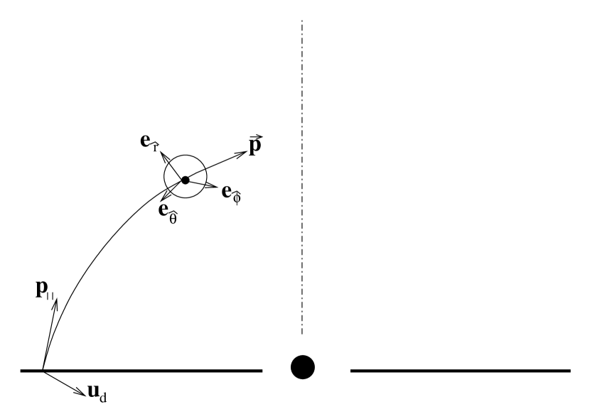
Figure 1: The geometry behind the computation of the total momenergy deposition rate in the observer’s orthonormal frame (hatted basis vectors).

The number densities $f_{\nu}$, $f_{\bar{\nu}}$ are Lorentz invariant and conserved along the $\nu$, $\bar{\nu}$ world lines (null geodesics). If $\bar{\mathbf{p}}=\langle\varepsilon,\mathbf{p}\rangle$ is the neutrino (anti-neutrino) 4–momentum in the observer frame ($\varepsilon=|\mathbf{p}|$), and $\bar{\mathbf{p}}_{\parallel}=\langle\varepsilon_{\parallel},\mathbf{p}_{\parallel}\rangle$ is the 4–momentum of the same neutrino in the comoving frame of the disk at the point of emission ($\varepsilon_{\parallel}=-\bar{\mathbf{u}}_{e}\cdot\bar{\mathbf{p}}_{\parallel}$) then $f_{\nu}$ is computed as

$$f_{\nu}=f_{\nu}(\mathbf{p}_{\nu},\ldots)=\frac{I_{\nu}}{\nu^{3}}\left(\frac{1}{h^{4}}\right)=\frac{2}{h^{3}}\left({\mathrm{e}}^{\varepsilon_{\parallel\nu}/kT}+1\right)^{-1}$$ (20)

where $I_{\nu}$ is the specific intensity of radiation at a given frequency $\nu$. Note that the ratio $\frac{I_{\nu}}{\nu^{3}}$ is Lorentz invariant by Liouville’s Theorem. The value of $\varepsilon_{\parallel\nu}$ in this equation is determined by the 4–momentum of the neutrino parallel translated to the disk along the world line of the neutrino $\mathbf{p}_{\parallel\nu}$ and on the 4–velocity of the particle in the disk emitting the neutrino $\bar{\mathbf{u}}_{e}$. The latter is computed as

$$\bar{\mathbf{u}}_{d}=\langle u^{t},0,0,u^{\phi}\rangle=\left\langle\frac{dt}{d\tau},0,0,\frac{d\phi}{d\tau}\right\rangle=\frac{dt}{d\tau}\,\left\langle 1,0,0,\frac{d\phi}{dt}\right\rangle$$ (21)

where[15]

$$\frac{d\phi}{dt}=\Omega=\frac{M^{1/2}}{r^{3/2}+aM^{1/2}}$$ (22)

for the direct circular orbit of the emitting particle.

The normalization condition

$$\bar{\mathbf{u}}_{d}\cdot\bar{\mathbf{u}}_{d}=-1$$ (23)

written as

$$\left(\frac{dt}{d\tau}\right)^{2}\left(g_{tt}+2g_{t\phi}\,\Omega+g_{\phi\phi}\,\Omega^{2}\right)=-1$$ (24)

allows the evaluation of $u^{t}$ as

$$u^{t}=\frac{dt}{d\tau}=\left[-\left(g_{tt}+2g_{t\phi}\,\Omega+g_{\phi\phi}\,\Omega^{2}\right)\right]^{-\frac{1}{2}}$$ (25)

The value of $\bar{\mathbf{u}}_{d}$ is given by

$$\bar{\mathbf{u}}_{d}=\left\langle u^{t},0,0,u^{t}\,\frac{d\phi}{dt}\right\rangle$$ (26)

The steps for evaluating $f_{\nu}(\vec{p})$ are as follows:

1. $\vec{p}\longrightarrow\mathbf{p}_{\nu}=\langle|\vec{p}|,\vec{p}\rangle$ in the frame of observer (supplied by the integrating program)

2. $\mathbf{p}_{\nu}=\langle p^{t},p^{r},p^{\theta},p^{\phi}\rangle$ Transformation to global coordinates

3. Tracing geodesics starting at $(t,r,\theta,\phi)_{obs}$ tangent to $\mathbf{p}_{\nu}$ to the disk. Pick the geodesic parameter $\lambda$ such that $\frac{d}{d\lambda}=\mathbf{p}_{\nu}$, integrate back to $\theta=\frac{\pi}{2}$ ($\lambda=0$ at the observer, $\lambda<0$ at the disk). This procedure yields $(t,r,\theta,\phi)_{disk}$ and $\mathbf{p}_{\parallel\nu}=(d/d\lambda)_{disk}=\langle p^{t},p^{r},p^{\theta},p^{\phi}\rangle_{disk}$

4. Computing $\bar{\mathbf{u}}(t,r,\theta,\phi)_{disk}=\bar{\mathbf{u}}_{d}$

5. Computing $\varepsilon_{\parallel}=-\bar{\mathbf{u}}_{d}\cdot\mathbf{p}_{\nu}$

6. Computing $f(\vec{p})=f(\varepsilon_{\parallel})$ using equation (20)

Assuming the emission rates of the neutrinos and the anti-neutrinos at the disk are identical, and assuming the neutrinos are emitted isotropically as a Planck black-body spectrum characterized by the temperature $T_{disk}$ in the frame comoving with the disk material, then the spectrum of neutrinos that our observer sees is also a Planck spectrum. However, the temperature characterizing our observer’s spectrum is scaled by the frequency shift of the neutrinos.

$$T_{\cal O}=\frac{\varepsilon_{\cal O}}{\varepsilon_{\parallel}}T_{disk}$$ (27)

Following the derivation of Salmonson and Wilson[12], the MDR integral (Eq.19) can be transformed into a 4-dimensional integral by analytically integrating over $\varepsilon_{\nu}$ and $\varepsilon_{\bar{\nu}}$.

$$MDR=\frac{7\pi^{3}\zeta(5)DG_{F}^{2}}{2h^{6}}\int\limits_{\nu}\int\limits_{\bar{\nu}}(k{{\bar{T}}_{\cal O}})^{4}(kT_{\cal O})^{5}(\mathbf{\Omega}_{\nu}\cdot\mathbf{\Omega}_{\bar{\nu}}-1)^{2}\mathbf{\Omega}_{\nu}\,d\Omega_{\nu}\,d\Omega_{\bar{\nu}}$$ (28)

Here, the temperature ${T}_{\cal O}$ is the temperature of the black body spectrum of the neutrinos as measured by the observer ${\cal O}$. It will ordinarily depend on both the sky angles ($\psi$, $\xi$) we integrate over. In a similar way ${\bar{T}}_{\cal O}={\bar{T}}_{\cal O}({\bar{\psi}},{\bar{\xi}})$. Using Eqn. 27 we can rewrite the momenergy deposition rate in terms of the disk temperature.

$$MDR=\alpha I(r_{\cal O},\theta_{\cal O})$$ (29)

where $r_{\cal O}$ and $\theta_{\cal O}$ are the BL coordinate location of the observer, the integral function is driven by the redshift of the neutrinos and anti-neutrinos arriving at the observer,

$$I(r_{\cal O},\theta_{\cal O})=\int\limits_{\nu}\int\limits_{\bar{\nu}}\left(\frac{{\bar{\varepsilon}}_{\cal O}}{{\bar{\varepsilon}}_{\parallel}}\right)^{4}\left(\frac{\varepsilon_{\cal O}}{\varepsilon_{\parallel}}\right)^{5}(\mathbf{\Omega}_{\nu}\cdot\mathbf{\Omega}_{\bar{\nu}}-1)^{2}\mathbf{\Omega}_{\nu}\,d\Omega_{\nu}\,d\Omega_{\bar{\nu}}$$ (30)

and the constant $\alpha$ depends strongly on the temperature of the disk as measured by the Keplerian observer.

$$\alpha = \frac{7\pi^{3}\zeta(5)DG_{F}^{2}}{2h^{6}}\left(kT_{disk}\right)^{9}$$ (31)

$$= 1.84\times 10^{32}\ \left(\frac{kT_{disk}}{10MeV}\right)^{9}\ \frac{ergs}{sec-cm^{3}}$$

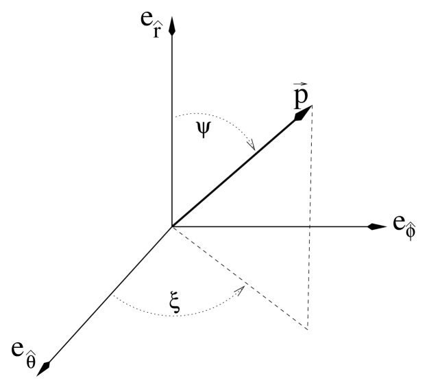
Figure 2: Spherical coordinate sky angles ($\psi$ and $\xi$) used, in part, to generate the 4-momentum $\mathbf{p}$ in the observers rest frame.

In order to calculate the generation of 4-momentum from the $\nu$–$\bar{\nu}$ scattering, we must first image the accretion disk in the observer’s reference frame. We do this by using a full 3-dimensional ray-tracing code for a Kerr spacetime. The input needed by the ray-tracing code in order to image a given pixel of the disk is the location of the observer (${\cal O}=\{t,r,\theta,\phi\}$) and the components of the 4-momentum ($\mathbf{p}$) in Boyer-Lindquist coordinates.

$$\mathbf{p} = p^{\hat{0}}\mathbf{e}_{\hat{0}}+p^{\hat{r}}\mathbf{e}_{\hat{r}}+p^{\hat{\theta}}\mathbf{e}_{\hat{\theta}}+p^{\hat{\phi}}\mathbf{e}_{\hat{\phi}}$$

$$= p^{0}\mathbf{e}_{0}+p^{r}\mathbf{e}_{r}+p^{\theta}\mathbf{e}_{\theta}+p^{\phi}\mathbf{e}_{\phi}$$

We can express the 4-momentum of the neutrino in the observer’s frame by using the two spherical sky angles ($\psi$ and $\xi$) shown in Fig. 2.

$$p^{\hat{0}} = |\vec{p}|\ =\ \varepsilon_{\nu}$$

$$p^{\hat{r}} = |\vec{p}|\cos{(\psi)}$$

$$p^{\hat{\theta}} = |\vec{p}|\sin{(\psi)}\cos{(\xi)}$$

$$p^{\hat{\phi}} = |\vec{p}|\sin{(\psi)}\sin{(\xi)}$$

The magnitude of the 3-momentum ($|\vec{p}|$), and the time component of the 4-momentum, were obtained by assigning an energy to the neutrino in the observers frame ($\varepsilon_{\nu}$) and using the normalization condition, $\mathbf{p}\cdot\mathbf{p}=0$. We can recover these components in the Boyer-Lindquist coordinates by inverting Eqns.(11,12,13,14).

$$p^{t} = \frac{\varepsilon_{\nu}}{\sqrt{-g_{tt}}}-\sqrt{\frac{g_{tt}}{g_{\phi\phi}g_{tt}-g_{t\phi}^{2}}}\ \left(\frac{g_{t\phi}}{g_{tt}}\right)\ \varepsilon_{\nu}\sin{(\psi)}\sin{(\xi)}$$

$$p^{r} = \frac{\varepsilon_{\nu}}{\sqrt{g_{rr}}}\cos{(\psi)}$$

$$p^{\theta} = \frac{\varepsilon_{\nu}}{\sqrt{g_{\theta\theta}}}\sin{(\psi)}\cos{(\xi)}$$

$$p^{\phi} = \sqrt{\frac{g_{tt}}{g_{\phi\phi}g_{tt}-g_{t\phi}^{2}}}\ \varepsilon_{\nu}\sin{(\psi)}\sin{(\xi)}$$

To reconstruct the image of the entire disk at ${\cal O}$, we integrate over all values of the sky angles ($\psi\in\{0,\pi\}$ and $\xi\in\{0,2\pi\}$). We use the ray-tracing code[16] to calculate the 4-momentum of the neutrino ($\mathbf{p}_{\|}$)when it hits the disk.

In Fig. 3 we provide an illustrative example of the imaging of an accretion disk extending from $r\approx 4.233M$ (the inner-most stable orbit of a Kerr black hole of mass $M$ and specific angular momentum $a=0.5$) out to $r=10M$. Here the observer ${\cal O}$ is located at BL coordinates $r=8M$ and $\theta=3\pi/8$. The image of the disk is color coded as to the energy of the neutrinos reaching the observer. This image is used to calculate the MDR (Eqn. 28). We also provide a convergence plot for the MDR in Fig. 4.

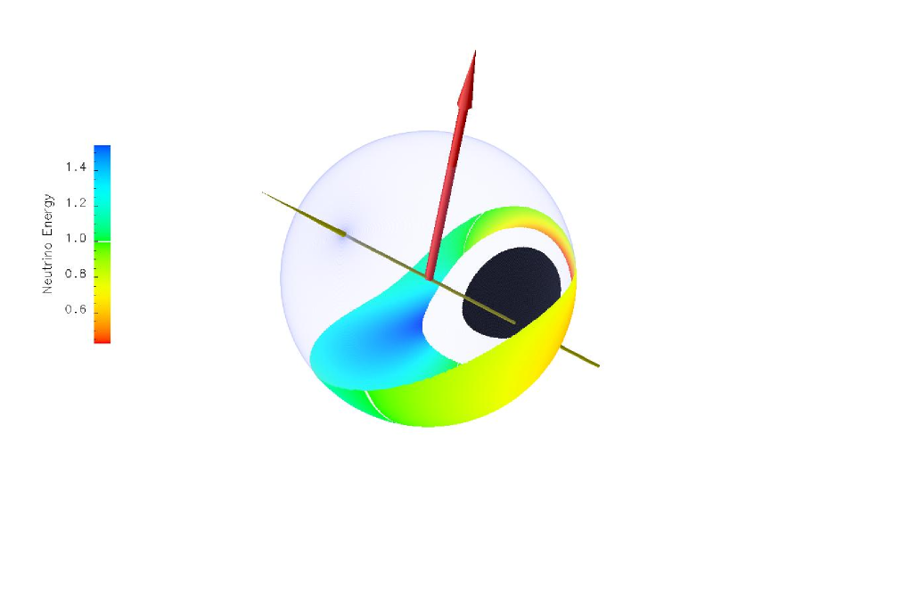
Figure 3: A color rendering of the sky map of an observer located above a rotating ($a=0.5$) black hole of mass ($M$). The observer is located a distance $8M$ from black hole at an inclination $\theta=3\pi/8$. The thin Keplerian accretion disk extends from the inner-most stable orbit ($r\approx 4.233M$) out to $r=10M$. We assume that the neutrinos are emitted from an isothermal disk of temperature $T_{disk}=1$ (as measured by the local comoving Keplerian observers). The spectrum of the neutrinos and anti-neutrinos are assumed to be a Planck spectrum characterized by this temperature. The long thin yellow-colored coordinate axis represents the observer’s orthonormal ${\hat{r}}$ coordinate axis. The thicker red arrow originating from the center of the observer’s celestial sphere represents the sum of all the scattered momenergy as projected on the observer’s spatial frame. The image of the accretion disk is shown color coded by the energy of the arriving neutrinos as measured in the observer’s frame. In particular, the thin white, saturated band on the disk image represents zero frequency shift. The neutrinos from the blue region (darker region on the back of the sphere) are blue shifted due to the closing relative velocity of the observer and the rotating disk material, and the reddened regions indicate the gravitational red shift effect from the black hole. The non-axial symmetry of the disk image, black hole and region between the horizon and the inner edge of the disk is due to the black hole’s rotation (i.e. Lense-Thirring effect, frame dragging or gravitomagnetism). This image was generated using a grid on the sphere of dimensions $800\times 1600$.

Figure 4: A demonstration of the convergence of the energy deposition rate and tilt of the scattered electrons/positrons as a function of the number of pixels used to image the accretion disk. In this particular convergence test, we use an observer located at $r=8M$ and $\theta=7\pi/16$ in an ($a=0$) Schwarzschild spacetime. We chose the location of this observer to correspond to the region of maximal momenergy production (as shown in the next figure). We plot the scattering integral $I$ in the left plot, and the angle $\psi$ in the right plot as a function of the number of grid points used to resolve the accretion disk. The maximum resolution used in this convergence test involved tracing $2\times 10^{6}$ geodesics over the entire celestial sphere. Of these geodesics, approximately one in seven, or $3\times 10^{5}$, hit the disk.

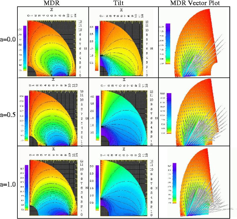
Figure 5: Pictorial representation of our simulations for three values of the spin of the black hole. The first row represents a Schwarzschild black hole ($a=0$), while the third row an extreme Kerr hole ($a=1$). The second row represents our results for a moderately rotating black hole ($a=0.5$). The accretion disk in each of these cases extend from $10M$ in toward the black hole down to the inner-most stable orbit. The first column shows a contour plot of the magnitude of the time component of the momenergy deposition rate in Kerr coordinates, the second column depicts a contour plot of the angle, or tilt, the spatial components (in Boyer-Lindquist coordinates) of the MDR make with the symmetry $z$-axis. In the third column, we combine the information in the first two columns and pictorially show the spatial Boyer-Lindquist components of the momenergy deposition rate for various locations about the black hole accretion disk system. One can observe the dominant contribution to the MDR above the surface of the disk produced by the $\nu\bar{\nu}$ collisions as well as their pitch angle. Values of the MDR can be obtained by multiplying the numbers in the graph by $\alpha$ and by the cube of the black hole’s mass.

6 Estimate of the Transport of the Momenergy out to the Jet-Producing Region

Up to this point we have calculated the total momenergy density created in a given observer’s orthonormal frame per unit 3-volume per unit proper time. These results are posed properly in general relativity as they represent a meaningful local observation. However, for the GRB application we address in this paper it would be useful to determine the electron distribution function for an observer at large radii (e.g. $r=50M$) from the accretion disk. This location would approach the inner envelope of a hypothetical stellar shell surrounding the black-hole/accretion disk system. At such a location we could construct a source term for the fluid at the inner envelope of the star that would provide the energy for a jet which would ultimately punch through the outer atmosphere of the star – a jet that would be the generator of a fireball-type solution. Unfortunately, the construction of such a source is a computationally difficult problem even under the ideal assumptions that the electrons created evolve as a collisionless fluid and are highly energetic ($E\gg m_{e}$). If we want to know how many electrons with momentum $p$ arrive at an observer located at spacetime event $x$, then we would need to construct the geodesic into the past tangent to $p$ at $x$ and sum up the electron creation functions along and tangent to that geodesic.[17] This would require modifying the calculation of the MDR (Eq. 15) to calculate the probability distribution functions for the creation of electrons at each point. We would then need to construct and store these electron creation functions on a dense grid in the $z$-$x$ plane perpendicular to the disk and integrate these creation distribution functions over the 3-parameter (2 sky angles and electron energy defining $p$) family of geodesics of the observer at $x$. Alternatively, we could solve a 3-dimensional collisionless Boltzmann equation for the Kerr spacetime geometry.[18] Unfortunately, both of these approaches, while correct in a GR sense, are computationally demanding in the extreme. While there is no technical reason that would prevent us from carrying out these calculations, practical considerations prevent us from completing them in the near future. Consequently, we elect to pursue a simpler computational strategy for the estimation of the GRB jet source term.

The difficulties with a general covariant treatment originate with the Kerr black hole and not with the Schwarzschild solutions. In particular, we currently calculate the total 4-momentum deposited per unit 4-volume in the observer’s orthonormal frame. Any attempt to assign a 4-volume to the observer in BL coordinates (or any coordinate) would break general covariance. In other words, the spatial slices of the BL metric are not orthogonal to the time lines ($g_{\phi t}\neq 0$), and thus the 3-space of our observers is not integrable. Nevertheless, if we take the total MDR calculated in the last section and transform this to the BL coordinates and multiply by the “effective BL spatial 3-volume” of our observer, we can obtain an approximation to a 4-momentum per proper time of electrons created at that location. This is a coordinate-dependent quantity which should be adequate for a qualitative understanding as long as the observers are not too close the the horizon of a rotating black hole. Moreover, electron-positron production close to the horizon should not be expected to contribute significantly to the results at large radii, as the electron-positron production for observers close to the horizon will be dominated by in-scatter of the electrons and positrons into the black hole. Given coordinate dependent MDR quantities, we then parallel transport each of these 4-dimensional momenergy vectors parallel to themselves out to the inner shell of the collapsar (say at $r=50M$). We then determine the time dilation and bin the results as a function of the poloidal angle. In this way we can estimate the MDR from neutrino scattering as a function of the angular momentum of the black hole.

This treatment is obviously non-covariant. However, as the astrophysical uncertainties of the environs of such a black hole/accretion disk system appear to be, at present, far greater than the issues with relativity we raise here; we feel that our violation of general covariance to simplify the computational requirements may be justified in order to provide at least a qualitative understanding of the off-axis energy-deposition at the inner envelope. We acknowledge that for a more complete characterization of the source term, a covariant treatment should ultimately be undertaken. In the meantime, we feel that the results presented herein provide a useful qualitative estimate.

We have provided a pictorial representation of the total MDR calculated for a field of observers in the $z$-$x$ plane perpendicular to the accretion disk in Fig 5. Here we have placed $10^{4}$ observers in this plane and calculated the MDR for each using Eq. (28). The observers were evenly spaced in 100 equal BL increments ($\Delta r$) in radius from $r=2.5M$ out to $r=12M$, and equally spaced in 100 BL poloidal increments ($\Delta\theta$) from $\theta=0$ to $\theta=\pi/2$. The MDR densities were transformed to BL coordinates. The 3-volume assigned to each observer is, as mentioned above, coordinate dependent ($\Delta V=2\pi\sqrt{g_{ij}}\Delta r\Delta\theta$) The last column of the figure illustrates the structure of the MDR generated above the surface of the accretion disk.

In Fig. 6 we integrated the BL MDR 4-momentum out along their geodesics until they either hit the black hole or they reach $r=50M$. We do this for five black hole/disk systems. The five systems correspond to specific angular momentums with the values, $a=0.0,0.25,0.5,0.75\ \mbox{and}\ 1.0$. For each value of $a$ the BL time component of the MDR in the BL frame reaching $r=50M$ was binned into 20 bins ranging from $\theta=0$ to $\theta=\pi/2$. The relative magnitude of these curves increase with increasing values of the specific angular momentum of the central black hole. We have investigated the origin of this increase and find that the source of the increase is the region of the accretion disk near the inner-most stable orbit. This is illustrated in (Fig. 7) where we compare the angular MDR profile for an accretion disk extending from $6M$ out to $10M$ with (1) a Schwarzschild black hole and (2) and extreme Kerr black hole. The magnitudes are approximately equal and only a slight tightening of the angle of the peak MDR is apparent for the extreme Kerr black hole system.

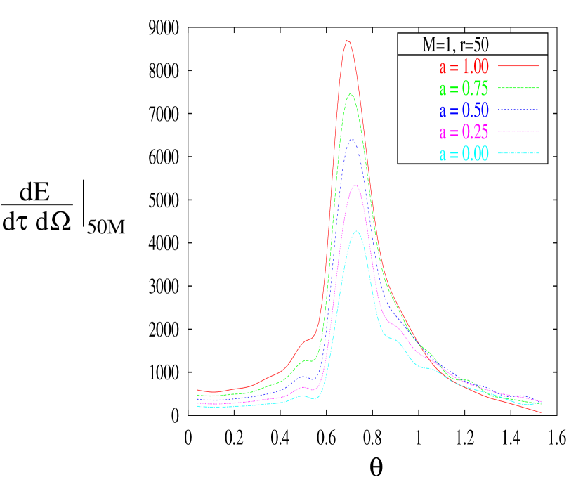
Figure 6: We bin the MDR per unit solid angle as a function of the poloidal angle ($\theta$) at $r=50M$ for black hole/accretion disk systems with five values if the specific angular momentum ($a=0,.25,.5,.75\ \mbox{and}\ 1$). Although $dE/d\tau d\Omega$ levels off and yields results consistent with the conjecture of AF that the MDR is constant for small angles away from the axis; nevertheless, we do find a substantial disk-driven wind source off-axis. We demonstrate here the following two features: (1) The largest contribution to the MDR originates just above the disk giving factors of 10 to 20 above the on-axis non-relativistic contributions calculated by others. This gives rise to a disk-driven wind. This wind, when propagated out to $r=50M$ along geodesics produces the peak in the MDR profiles shown in the figure. This peak corresponds to depositing the bulk of the MDR in a cone with opening angle $\theta\approx\pi/4$; and (2) The MDR only mildly depends on the specific angular momentum of the disk and in an approximately linear fashion. The excess MDR for the extreme Kerr system results from the size of the accretion disk. In the Kerr system the disk extends from just above $r=M$ out to $r=10M$; however, in the Schwarzschild case the disk extends from $r=6M$ out to $r=10M$. These runs were performed using $10^{4}$ observers located at constant $\delta r$ and $\delta\theta$ intervals in the $z$-$x$ plane. The observers were placed between $r=2.5M$ and $r=10M$. The MDR integral was calculated at each of these observers using $2\times 10^{4}$ grid points covering the celestial sphere. Values of the MDR can be obtained by multiplying the numbers in the graph by $\alpha$ and by the cube of the black hole’s mass.

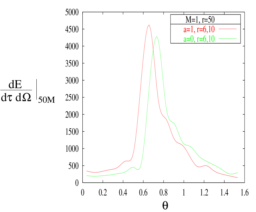
Figure 7: Demonstration that the MDR is primarily driven by the size of the disk and thus the location of the inner-most active region (active in the sense of neutrino production) of the accretion disk. In the previous figure (Fig. 6) we saw a factor of two increase in the peak MDR for an extreme Kerr black hole as compared to the Schwarzschild system. This is because the disk around the Kerr black hole extended down to the horizon, while in the Schwarzschild spacetime the disk ended at the inner most stable orbit at $r=6M$. In this figure we compare these two systems with the same disk. In both simulations ($a=0$ and $a=1$) we use an isothermal accretion disk with inner and outer radii of $6M$ and $10M$, respectively. However, one simulation uses an extreme Kerr black hole ($a=1$), while the second simulation uses a Schwarzschild hole ($a=0$). The effect of angular momentum, sans location of the inner most stable orbit, has a marginal effect on both the magnitude of the total momenergy deposited at $50M$ and on the direction of the momenergy. Values of the MDR can be obtained by multiplying the numbers in the graph by $\alpha$ and by the cube of the black hole’s mass.

We demonstrate convergence of our results with regard to the number of observers we use in the $z$-$x$ plane by comparison of a high and lower resolution run (Fig. 8). The higher resolution, which we use in our calculations in this manuscript, is a little smoother than the lower resolution run; however, the both compare well with each other.

Figure 8: Demonstration of the convergence of our calculations of the MDR at $50M$ using different number of observers located in the $z$-$x$ plane around an $M=1$ Schwarzschild black hole/accretion disk system. The high resolution curve uses $1.5\times 10^{4}$ observers in the $z-x$ quadrant(equally spaced between $r=2.5M$ and $r=12M$), while the low resolution curve uses $1\times 10^{4}$ observers in this quadrant. In both cases the MDR scattering integral used $100\times 200$ grid points. Here we plot the MDR per unit $\theta$ as opposed to MDR per unit $\Omega$ in the other figures. Values of the MDR can be obtained by multiplying the numbers in the graph by $\alpha$ and by the cube of the black hole’s mass.

The relevant quantity reported by AF was the total MDR at a distant observer. If we integrate each of the five MDR curves shown in Fig. 6 over $\Omega$ at $r=50M$ we will obtain the integrated MDR into the jet as shown in Fig. 9. It will be concentrated along the axis and peak along a cone of opening angle $\pi/4$. This opening angle is due to the tilt of the MDR near the surface of the disk. The tilt is in the direction of the disk’s rotation. We find a linear dependence for this integrated MDR as a function of the specific angular momentum of the black hole. This is an extension of the earlier results because we are including the relatively large off-axis source term – the MDR created just above the surface of the disk via $\nu$ $\bar{\nu}$ scattering. This disk MDR produces a 10 to 20 fold enhancement to the total MDR energy deposited at $r=50M$ over and above the on-axis MDR, even for a Schwarzschild black hole. Such a disk-generated MDR was also found in the non-gravitational models of AF.[11] The dependence of this disk-driven source of momenergy on the specific angular momentum of the black hole is roughly linear. We predict a twofold increase in the MDR for an extreme Kerr black hole relative to a Schwarzschild hole. In addition, in (Fig. 6) we only see a slight tightening of the cone of the momenergy deposition with increasing $a$. It would be interesting to observe the jet dynamics through the outer envelope of the star with sources of this kind.

Figure 9: We plot the total BL time component of the MDR at $50M$ as a function of five values of the specific angular momentum ($a$) of a solar-mass black hole with a 10 MeV temperature accretion disk. In other words, we integrate each of the five profiles in Fig. 6 over the solid angle $\Omega$. This shows that the MDR is roughly a linear function with respect to the specific angular momentum ($a$) of the black hole. We provide a least-squares fit of the five numerical points. The integration of the MDR profiles are done over the entire northern hemisphere. If we integrated our profiles only over a small solid angle around the symmetry axis we would find our result are consistent with those reported by AF. However, we include here the disk-driven wind created by $\nu$–$\bar{\nu}$ scattering above the disk’s surface. We see a large factor (approximately 10-20 times) in the MDR from the disk surface over and above the on-axis source calculated by AF and SW. This enhancement occurs equally well for Schwarzschild black holes as for Kerr black holes.

7 Conclusions: Enhancement of the Energy Deposition from a Disk-Driven Wind

The goal of the research in the GRB central engine modeling community over the last few years was to look for a needed enhancement of a factor of 10 in the MDR. Previous work by AF and SW looked for such an enhancement over the non-gravitating models by examining the GR effects on neutrino pair scattering along the symmetry axis. They did not find this enhancement; however, in this paper we identify the off-axis disk-driven MDR component that yields such an increase over corresponding on-axis MDR values. Furthermore, this disk-driven momenergy occurs in the non-rotating black holes as well as the rotating black holes, and is even present in the non-physical models with no gravity effects (e.g. Fig 4 of Ref. [11]). We therefore have strong indication that the the current fireball central engine model discussed here is viable. Of course, more detailed astrophysical simulations are needed which include the complex environs of the black hole disk system, geometry and transient behavior of the disk and black hole, and a simulation of the induced plasma transport of the scattering out to the fireball region. Since this disk-driven MDR source is relatively large, and since the baryon pollution problem[19] remains an open issue in this field,[1] we argue that it may be premature to discount this off-axis source. We should reserve such a decision until more detailed GR, hydrodynamic, MHD and plasma transport calculations have been done.

As we outlined in the paper, we have extended the earlier work of AF to calculate the off-axis contribution to the MDR. When using the assumptions made by these authors, our results are consistent their work; however, we find the generation of a substantial MDR above the disk, which, when added to the on-axis calculations of these authors produce a substantial enhancement to the deposition of energy-momentum. In particular, we find an approximately linear dependence of the total MDR at large $r$ as a function of specific angular momentum of the black hole.

$$\left.\frac{dE}{d\tau}\right|_{50M}\approx 4.06\times 10^{51}\ \left(1+.73a\right)\ \left(\frac{kT_{disk}}{10MeV}\right)^{9}\left(\frac{M}{M_{\odot}}\right)^{3}\ \frac{ergs}{sec}$$ (32)

Here we did a least-squares fit to the numerical results in Fig. 9, multiplied by $\alpha$ times the cube of the solar mass ($M_{\odot}=1.47\times 10^{5}cm$). The bulk of the MDR at large $r$ is deposited in a conic region centered on the symmetry axis of the system with an opening angle of approximately $\pi/4$.

Although we provide a rigorous general relativistic calculation of the MDR at an arbitrary observer, computational constraints required us to make some approximations regarding the transport of the scattered energy out to the inner envelope ($r=50M$) of the star. Assuming (1) the electrons produced have substantially higher energy than their rest mass, (2) that the electrons propagate away in a collisionless fashion and (3) that the observationally-relevant electron creation distribution functions are peaked around the total MDR calculated, then our results should be rigorously correct for a Schwarzschild black hole, and qualitatively correct for spinning black holes. We would not be surprised if a general-relativistically rigorous calculations would yield different quantitative results for the extreme Kerr black hole close to the horizon. However, one of the main results of this paper is the identification of the off-axis disk-driven MDR as providing an enhancement to the energy deposition rate rather than the GR-driven enhancements.

We outlined in the last section an approach to calculate the electron distribution function at an observer $\cal O$ at large $r$ in a relativistically covariant way. This involved integrating the electron-creation distribution functions along geodesics into the past which originated at $\cal O$. One step in this direction would be to extend the work here and calculate the electron creation distributions in the frame of our observers as opposed to the total MDR. This is not difficult in principle but is computationally demanding as it would require evaluating a 6-dimensional scattering integral as opposed to the 4-dimensional integral we evaluated numerically in Sec. 5, Eqn. 28. The utility of such a calculation would be to evaluate the point along the axis on the border between out-scatter and in-scatter (i.e. when the total MDR was zero). Would the electron creation function at and about this event yield a non-negligible contribution to the electron distribution function at large $r$?

On a more speculative note, we also are interested in calculating secondary scattering of the electrons and positrons within the ergosphere of the black hole. We have found evidence of significant in-scatter into this region. Will the Penrose process produce some observable high energy events from this region that can give us more clues to the inner workings of the central engine of these low mass black hole/accretion disk systems?

One question seems of paramount importance in this field: What observational features of a GRB can give clues as to the inner-workings of the central engine?[20] Surely future X-ray, $\gamma$-ray and gravity wave observatories complemented with theory can soon unveil these cosmic explosions.

8 Acknowledgments

We wish to thank Doug Eardley, Adrian Gentle, Bob Geroch, Daniel Holz and Rosalba Perna for stimulating conversations on this subject, and Chris Fryer for suggesting this problem. We thank the Institute for Theoretical Physics at UC Santa Barbara for providing a supportive and stimulating research environment to complete this research. This project was supported by Los Alamos under the LDRD/ER program and in part by the National Science Foundation under Grant No. PHY99-07949.

References

- [1] P. Mészáros Annu. Rev. Astron. Astrophys. 40 (2002).
- [2] G. Cavallo and M. J. Rees, M.N.R.A.S. 183 (1978) 359.
- [3] B. Paczyński, ApJ Lett. 308 (1986) L47.
- [4] A. Shemi and T. Piran, ApJ Lett. 365 (1990) L55.
- [5] S. E. Woosley, ApJ 405 (1993) 273.
- [6] R. Popham, S. E. Woosley and C. Fryer, ApJ 518 (1999) 356.
- [7] D. Eichler, M. Livio, T. Piran and D. N. Schramm, Nature 340(1989) 126.
- [8] A. MacFadyen and S. E. Woosley, ApJ 524 (1999) 262.
- [9] M. Vietri, G. Perola, L. Piro and L. Stella, MNRAS 308 (2000) L29.
- [10] K. Asano and T. Fukuyama, ApJ 546, (2001) 1019.
- [11] K. Asano and T. Fukuyama, ApJ 531, (2000) 949.
- [12] J. D. Salmonson and J. R. Wilson, astro–ph/9908017 (1999)
- [13] J. A. Wheeler, Journey into Gravity and Spacetime (W. H. Freeman & Co., San Francisco, Scientific American Library, No. 31, 1990)
- [14] C. W. Misner, K. S. Thorne and J. A. Wheeler, Gravitation (W.H. Freeman & Co., San Francisco, 1973) p. 586.
- [15] J. M. Bardeen et. al., ApJ 178, 347 (1972)
- [16] B. Bromley, K. Chen and W. A. Miller, ApJ 475 (1997) 57.
- [17] B. Geroch, Private Communication in Los Alamos, 2001.
- [18] M. Liebendoerfer, A. Mezzacappa and F-K. Thielemann, Phys. Rev. D63 (2001) 104003.
- [19] B. Paczyński, ApJ 363 (1990) 218.
- [20] S. E. Woosley, ”Gamma-Ray Bursts: The Central Engine,” in Gamma-Ray Bursts in the Afterglow Era, Proceedings of the International workshop held in Rome, CNR headquarters, 17-20 October, 2000. eds. E. Costa, F. Frontera, and J. Hjorth (Berlin Heidelberg: Springer, 2001, p. 257).