Shell Shock and Cloud Shock: Results from Spatially-Resolved X-ray Spectroscopy with Chandra in the Cygnus Loop

Abstract

We use the Chandra X-ray Observatory to analyze interactions of the blast wave and the inhomogeneous interstellar medium on the western limb of the Cygnus Loop supernova remnant. This field of view includes an initial interaction between the blast wave and a large cloud, as well as the encounter of the shock front and the shell that surrounds the cavity of the supernova progenitor. Uniquely, the X-rays directly trace the shock front in the dense cloud, where we measure temperature $kT=0.03$ keV. We find $kT\approx 0.2$ keV in regions where reflected shocks further heat previously-shocked material. Applying one-dimensional models to these interactions, we determine the original blast wave velocity $v_{bw}\approx 330{\rm\,km\,s^{-1}}$ in the ambient medium. We do not detect strong evidence for instabilities or non-equilibrium conditions on the arcsecond scales we resolve. These sensitive, high-resolution data indicate no exceptional abundance variations in this region of the Cygnus Loop.

1 Introduction

Supernova remnants fundamentally drive the cycle of matter and energy in the interstellar medium. Supernova remnants (SNRs) mix newly-formed elements into the interstellar medium (ISM), and they may determine whether those elements remain gaseous or enter the solid phase in the form of dust grains. SNRs drive mass exchange between the different phases of the ISM. Each SNR individually consists of an expanding hot interior, which can evaporate surrounding cold clouds. The compression of the ambient medium behind the SNR blast waves sets the stage for future generations of star formation. The interaction between the ISM and the stars in it is reciprocal. The stellar progenitor is responsible for processing the local medium, which alters subsequent evolution of the shock front, while the immediate environment profoundly influences the evolution of an individual SNR.

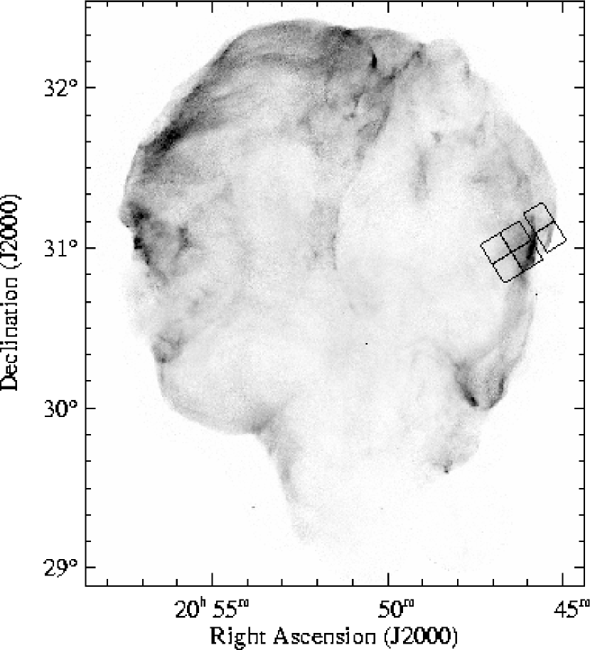
Figure 1: The context of these 31-ks Chandra observations is illustrated with the ACIS field of view overlaid on the ROSAT HRI mosaic of the Cygnus Loop (Levenson et al., 1997, completed with later observations). Interactions of the blast wave with large interstellar clouds produce the brightest X-ray regions. Forward blast wave propagation in the very dense cloud medium and the development of reflected shocks, which further heat and compress previously-shocked gas, together enhance X-ray emission at these locations.

The bright Cygnus Loop supernova remnant serves as an ideal probe of its surroundings (Fig. 1). It is middle-aged ($\tau=8000$ yr), with the extant ISM determining its subsequent evolution. Because the Cygnus Loop is nearby (440 pc; Blair et al. 1999), high spatial resolution, high signal-to-noise observations with the Chandra X-ray Observatory (Chandra) reveal hydrodynamical evolution of the blast wave and directly probe the inhomogeneous ambient ISM. Large clouds and a smooth atomic shell together define the boundary of the cavity the SNR’s progenitor created (Levenson et al., 1998), and shocks associated with both the cloud and shell produce X-rays, which we analyze here.

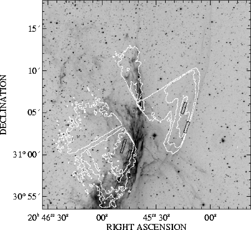
Figure 2: H$\alpha$ image of the western limb of the Cygnus Loop, on a logarithmic scale (Levenson et al., 1998). Fully radiative shocks produce the bright emission at the center of the field, while Balmer-dominated shocks trace the blast wave at the faint filaments toward the west. Contours of Chandra X-ray emission (white), also scaled logarithmically, and the spectral extraction regions (black rectangles) are overlaid. Some of the CCD boundaries are evident in the X-ray contours.

The brightest regions of the Cygnus Loop in optical and X-ray emission, such as the western and northeast limbs, are sites of interactions between the SNR blast wave and large interstellar clouds, which extend over scales of 10 pc. The blast wave is decelerated in the dense clouds. The shocks that advance in the clouds are radiative, and their cooling gas emits strongly in many optical lines, including hydrogen Balmer lines, [O III], and [S II], with typical temperature $T\sim 10^{4}$ K. Figure 2 illustrates the Cygnus Loop’s characteristic bright H$\alpha$ emission due to these slow cloud shocks at the western limb. Shocks that are reflected off the cloud surfaces propagate back through previously-shocked material, further heating and compressing it. These reflected shock regions exhibit enhanced X-ray emission (Hester & Cox, 1986), with characteristic temperature $T\sim 10^{6}$ K.

The extreme western limb also includes a portion of the primary blast wave. Raymond et al. (1980) first identified its characteristic faint filaments in H$\alpha$ images and showed that H$\alpha$ and H$\beta$ are the only strong lines in a filament’s optical spectrum. These “non-radiative” shocks excite Balmer line emission through electron collisions in pre-shock gas that is predominantly neutral (Chevalier & Raymond, 1978; Chevalier, Raymond, & Kirshner, 1980), marking regions where the gas is being shocked for the first time. The excitation is confined to a narrow zone immediately behind the shock front, so these filaments delineate the outer edge of the blast wave. This true boundary of the SNR is now located in the neutral shell of material at the edge of the cavity the progenitor star created.

The western limb is the archetype of cloud–blast-wave encounters in the Cygnus Loop. The large obstacle is detected directly in molecular observations (Scoville et al., 1977). More importantly, at this location we view the collision with the cloud nearly edge-on (Levenson et al., 1996). The stratification of the forward and reflected shock regions is therefore clear, and the simplification to a one-dimensional hydrodynamical problem on small resolved angular scales is reasonable. The X-ray data we present here also reveal the similar interaction of the primary blast wave with the cavity shell, allowing comparison of these effects in different interstellar conditions.

2 Observations and Data Reduction

We obtained a 31 ks exposure of the western limb of the Cygnus Loop on 2000 March 13 and 14 with the Chandra Advanced CCD Imaging Spectrometer (ACIS). (See Weisskopf et al. 2000 and the Proposers’ Observatory Guide at http://asc.harvard.edu/udocs/docs/docs.html for more information on Chandra and ACIS.) The total field of view is approximately $25\arcmin\times 17\arcmin$, with spatial resolution around $1\arcsec$ and simultaneous spectral resolution $E/\Delta E\approx 12$. We illustrate the X-ray context of these observations in Figure 1, marking the fields of view from the six Chandra detectors on the ROSAT High Resolution Imager (HRI) soft X-ray mosaic of the entire SNR. The presence of a large interstellar cloud enhances emission and indents the spherical blast wave here.

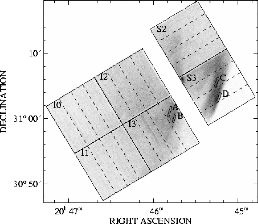
Figure 3: Chandra ACIS image of the western limb. This 0.1–8 keV image has been smoothed by FWHM$=3\arcsec$ and is scaled linearly from 0 (white) to 7 (black) total counts per $1\arcsec\times 1\arcsec$ pixel. The individual detectors are identified by name and marked with solid outlines. The approximate node boundaries are indicated (dashed lines). Rectangles (A–D) identify the regions for spectral analysis.

Figure 3 contains the total ACIS 0.1–8 keV image binned by a factor of two into $1\arcsec\times 1\arcsec$ pixels, with the detectors identified. This image is not corrected for existing large variations in detector sensitivity. The S3 CCD is oriented with its charge-transferring electrodes facing away from the incident X-rays, which greatly increases the soft X-ray sensitivity of this “back-illuminated” detector. The remaining five CCDs are “front-illuminated,” having readout electronics that face the incident photons and therefore absorb some of the soft X-rays from the astronomical source. The increased number of counts in the back-illuminated S3 CCD is the result of these differences, not varying emission intrinsic to the source. Within a given detector, each of the four readout amplifier nodes has a distinct spectral response, which produces smaller-magnitude variations; these node boundaries are also marked.

We reprocessed all data from original Level 1 event files, removing the 0.5-pixel spatial randomization that is included in standard processing. (See the Chandra Science Center at http://cxc.harvard.edu/ for details about Chandra data and standard processing procedures.) The latest gain files (from the Chandra calibration database, version 2.7, at http://cxc.harvard.edu/caldb/) were used to calibrate the back-illuminated S3 detector. During the first few months of Chandra operations, radiation damaged the front-illuminated devices, increasing their charge transfer inefficiency, consequently diminishing their spectral resolution and sensitivity. To mitigate these effects, we used the software and technique of Townsley et al. (2000), applying their response matrices for energy calibration. We included only good events that do not lie on node boundaries, where discrimination of cosmic rays is difficult. We examined the lightcurves of background regions and found no significant flares, so we did not reject any additional data from the standard good-time intervals.

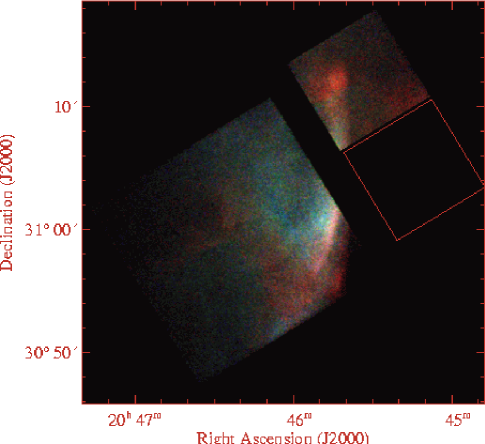
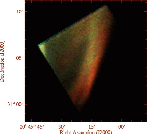
Figure 4: These false-color images reveal varying physical conditions over the field of view. Total counts in the 0.3–0.6, 0.6–0.9, and 0.9–2.0 keV energy bands are displayed in red, green, and blue, respectively, and the individual images have been binned by a factor of two and smoothed by FWHM$=14^{\prime\prime}$. The red square on the left indicates the location of the S3 detector (right), which is scaled differently because of its greater sensitivity at lower energies. (See §2 for details.) The softest (reddest) emission arises behind the decelerated blast wave as it propagates through the dense cloud and shell material. Reflected shocks produce corresponding hotter emission behind these slow shocks.

We combined three energy-selected images to create the false-color composite (Fig. 4). Total counts in the 0.3–0.6, 0.6–0.9, and 0.9–2.0 keV energy bands are displayed in red, green, and blue, respectively, and the individual images have been binned by a factor of two and smoothed by FWHM$=14\arcsec$. The individual energy images are not corrected for sensitivity variations within each detector or across the field. Thus, some of the color variation is not due to intrinsic spectral variation. Notably, because of its distinct spectral sensitivity as a function of energy, the correspondence between color and spectral shape in the back-illuminated S3 detector is different from that of the other five front-illuminated CCDs, so the S3 detector is displayed separately. Most importantly, the S3 detector is more sensitive at very soft X-ray energies. The component red, green, and blue images are scaled linearly from 0 to 2, 4, and 1.5, respectively, in the front-illuminated detectors, and to 5, 3, and 1, respectively, in the back-illuminated detector, in units of $10^{-7}{\rm photons\,cm^{-2}\,arcsec^{-2}}$.

3 Spectral Modeling

The false-color image (Fig. 4) illustrates significant spectral variation on small spatial scales within the Cygnus Loop. We identified several outstanding features (indicated in Fig. 3) that correspond to specific physical circumstances in the context of interactions between the SNR shock and the inhomogeneous ISM, as we demonstrate below. We extracted spectra from these small (roughly $1\arcmin\times 15\arcsec$) regions in order to isolate their particular spectral characteristics and to avoid calibration variations that are significant over larger areas. Within the bright emission of the I3 front-illuminated detector, the spectrum of region A is relatively hard, and that of region B is extremely soft. Immediately behind the primary blast wave observed on the S3 CCD, region C is spectrally harder than region D. Each spectral extraction was confined to a single read-out node of a detector, to avoid significant calibration variations that occur across node boundaries, and in each case, background emission was measured in an off-source region of the same CCD. Data were grouped into bins with a minimum of 20 counts, so $\chi^{2}$ statistics are appropriate in the model fitting.

We fit the spectra satisfactorily with thermal equilibrium plasma models. Specifically, we used the MEKAL model (Mewe, Gronenschild, & van den Oord, 1985; Arnaud & Rothenflug, 1985; Mewe, Lemen, & van den Oord, 1986; Kaastra, 1992), with updated Fe L calculations (Liedahl, 1992) in XSPEC (Arnaud, 1996). We used data in the energy range 0.3–2.0 keV from the back-illuminated detector and restricted the energy range to 0.4–2.0 keV from the front-illuminated CCD. The detector calibration uncertainties determined the lower energy bound, and the lack of significant emission above 2 keV in all instances set the upper bound. In all cases, we allowed temperature and absorbing column density to be free parameters. We constrained the latter $N_{H}\geq 4.7\times 10^{20}{\rm\,cm^{-2}}$, the column density that corresponds to the average visual extinction to the Cygnus Loop (Parker, 1967), which we assume is in the foreground, allowing for additional intrinsic absorption or variation as a function of position. Regions C and D do not require any additional absorption, so we fixed $N_{H}=4.7\times 10^{20}{\rm\,cm^{-2}}$ in their final spectral fits. Figure 5 shows the data, best-fitting models, and residuals for the four regions, and Table 1 lists the model parameters, corresponding emission measure, and count rates.

With one exception, a single temperature component is sufficient to describe the data with 99% confidence. In fitting the spectrum of region B, however, the inclusion of a second thermal component is statistically significant. As we describe below, this extraction does not cover the cooler cloud shock exclusively, but also contains an additional contribution along the line of sight from the hotter reflected shock, to which the detector is more sensitive. In all other cases, however, the addition of any second spectral component does not significantly improve the model fits.

In general, sub-solar oxygen abundance is necessary to fit the data, where $({\rm O/H})_{\odot}=8.51\times 10^{-4}$ (Anders & Grevesse, 1989). Because the characteristic temperatures we measure in the Cygnus Loop are very low compared with younger SNRs ($kT\leq 0.2$ keV), these spectra are particularly sensitive to oxygen, which accounts for nearly all the emission from 0.5–0.7 keV and represents a significant fraction of the detected photons. We examined the harder and softer portions of the spectra separately to confirm that they differ only in normalization and not temperature or ionization state, for example, so adjusting the oxygen abundance is reasonable. In the final modeling, we fixed the oxygen abundance at the best-fitting value for each detector, determined in the fitting of at least four spatially distinct extractions where the abundance was allowed to be a free parameter. We use ${\rm O/H}=0.53({\rm O/H})_{\odot}$ in the I3 CCD and ${\rm O/H}=0.44({\rm O/H})_{\odot}$ in the S3 detector. These values are similar to recent photospheric abundance measurements (e.g., Holweger, 2001).

We do not measure any systematic trend of abundance as a function of distance from the shock front, which indicates that we are not sensitive to the immediate effects of depletion and grain destruction in interstellar shocks. The offset, however, between the front-illuminated and back-illuminated CCDs is due to a difference in the relative soft-energy calibration of these detectors, not a physical variation over the spatial scale we investigate. We measure this calibration offset in a cloud interaction region that covers the S3 and I3 CCDs contiguously. The common physical conditions of this spatially-extended emission produce the same detector-specific abundance difference. Unfortunately, these observations are not strongly dependent on the abundances of elements that grain depletion affects most greatly. These data are not at all sensitive to silicon abundance, for example. At some of the higher observed temperatures ($kT\approx 0.2$ keV), we could measure depletion of iron at the 10% level, but because these hotter regions represent older shocked material, they are not physically revealing.

In addition to the broad oxygen complex, we note several other features in the spectra. Mg XI produces the emission near 1.35 keV in spectra from regions A and B. In the spectra of regions C and D, Ne IX transitions near 0.92 keV are obvious. In our final spectral analysis, we use the MEKAL model because it reproduces the prominent Ne emission significantly better than other equilibrium models. Qualitatively, the absence of Fe XVII emission around 0.73 and 0.83 keV emphasizes the relatively low temperatures of all the observed X-ray–emitting regions; these lines produce significant emission when $kT\geq 0.5$ keV.

We considered non-equilibrium ionization in the spectral modeling, which may be expected to be physically relevant to the conditions in the Cygnus Loop. Collisional ionization is not immediate following the shock, so the elements are initially under-ionized with respect to their equilibrium values. The ionization parameter, $n_{e}t$, characterizes the scale of equilibration, where $n_{e}$ is the initial electron density and $t$ is the time elapsed since the passage of the shock. Ionization equilibrium usually occurs when $n_{e}t\geq 3\times 10^{11}{\rm\,cm^{-3}\,s}$, depending on the element and its equilibrium state. The best fitting non-equilibrium ionization models tend toward equilibrium solutions, with $n_{e}t\gg 10^{12}{\rm\,cm^{-3}\,s}$. Furthermore, these non-equilibrium models do not statistically improve the spectral fits, so we do not consider them further here.

On physical grounds, we would expect non-equilibrium conditions to be marginally relevant. Using the densities and timescales calculated below (§4), we find $n_{e}t\sim 10^{12}{\rm\,cm^{-3}\,s}$, which is somewhat higher than previous results (e.g., Vedder et al., 1986; Miyata et al., 1994). At the very soft X-ray energies of the Cygnus Loop, however, no instrument has the spectral resolution and sensitivity on small spatial scales required to measure the non-equilibrium conditions directly and accurately. The spectra of a fully-equilibrated lower-temperature medium and the non-equilibrium state of a higher-temperature plasma remain indistinguishable. Thus, the adoption of the better-fitting equilibrium models in this analysis is justified.

In this inhomogeneous region, high spatial resolution is essential to derive physically meaningful conclusions from the spectral analysis. For comparison, we extracted the spectrum from a $2\arcmin$ circular region of the bright emission observed with the I3 detector. None of the models we applied, including multiple temperatures and non-equilibrium, fit this spectrum adequately because it covers such a range of physical conditions. We note that similar to analysis of ASCA spectra of other locations in the Cygnus Loop at comparable spatial resolution, extreme abundance variations are statistically preferred (Miyata & Tsunemi, 1999). The sensitive Chandra data, however, make clear that such exceptional models are still unacceptable, and they emphasize that spatially-integrated spectra do not directly measure genuine abundance variations.

4 Physical Interpretation

4.1 Cloud Shock

These Chandra data reveal the propagation of the SNR blast wave through the inhomogeneous ISM at the western limb of the Cygnus Loop. Over most of this region, we observe the interaction with a large interstellar cloud at the boundary of the pre-supernova cavity (Scoville et al., 1977). When the blast wave encounters the cloud, three characteristic regions become important: the decelerated forward shock in the cloud, a reflected shock, which propagates back through the previously-shocked ambient ISM, and the singly-shocked SNR interior (Hester & Cox, 1986). Because we view the plane of the shock nearly edge-on, the stratification of the spatially distinct emission regions is preserved. (See fig. 7 of Levenson et al. 1996 for a cartoon illustration of the geometry of this region.)

The distinct, narrow, pink feature in Figure 4, which extends over several arcminutes from north to south, directly illustrates the shock front in the cloud. Even though the cloud shock is slower than the undisturbed blast wave and will therefore not produce such hot plasma, the shock in the denser cloud produces very bright X-ray emission; for a given volume, emitted flux is proportional to $n^{2}$, where $n$ is density. The emission from the reflected shock region is also enhanced with respect to the rarefied singly-shocked SNR interior. The intense X-ray emission of this interaction was previously evident at the spatial resolution of the ROSAT HRI observations, but without simultaneous spectral information, the decelerated cloud shock and the harder reflected shock could not be distinguished. In these Chandra data, however, we uniquely identify both constituents of the X-ray enhancement. The location of the pink emission further identifies it as the cloud shock. It appears ahead of the harder reflected shock, and it is aligned with the onset of a radiative cooling zone observed optically (Fig. 2).

The peak emissivity of O VI occurs around the temperature of the shocked cloud, $T=3.5\times 10^{5}$ K, and oxygen is the dominant coolant at this temperature. Far-ultraviolet maps of the Cygnus Loop that are sensitive to the O VI doublet at $\lambda\lambda$1032, 1038 show strong emission at the western limb and are generally correlated with the X-rays (Blair et al., 1991; Rasmussen & Martin, 1992), consistent with O VI production in cloud shocks.

Because of the nearly edge-on geometry of this interaction, projection effects are not significant in this case, but they are present and explicable. For example, the emission slightly ahead (west) of the cloud shock yet still within the I3 CCD is due to another portion of the blast wave, which is likely on the near side of the cloud. The extremely soft (red in Fig. 4) patch near $\alpha=20^{\rm h}45^{\rm m}40^{\rm s}$, $\delta=30^{\circ}52\arcmin$ (J2000) of this region is associated with a fully radiative shock, detected at optical wavelengths in H$\alpha$ and [O III]$\lambda 5007$ lines. The relationship between multiple projections of the extended shock plane is expected when it encounters the non-uniform surface of an interstellar cloud. Another consequence of projection effects is that the spectral extraction of region B includes some contribution from the reflected shock in addition to the cloud shock along the line of sight. Qualitatively, this effect produces the pink cloud shock: the softest (red) emission is most significant, and combined with secondary harder (green and blue) contributions of the reflected shock along the line of sight, the net result is pink in this image. Chandra’s increasing effective area with energy up to 1 keV emphasizes this effect in the spectral extractions, and the spectral model of this region requires both the very soft emission of the slow forward shock and the hotter emission of the reflected shock that we measure in the spectrum of region A.

Distinguishing these two spectral components, we quantify the relationship between the shock velocities and density contrast of the cloud and cavity regions. For standard interstellar abundances, the post-shock temperature and cloud shock velocity $v_{c}$, are related by $T=1.4\times 10^{5}(v_{c}/100{\rm\,km\,s^{-1}})^{2}$ K. The measured temperature $T=3.5$ (+6.7, -1.9) $\times 10^{5}$ K corresponds to $v_{c}=150$ (+120, -40) ${\rm\,km\,s^{-1}}$. We solve the one-dimensional conservation equations of mass, energy, and momentum over both the cloud and reflected shock fronts, assuming constant pressure across the contact discontinuity that develops between the singly-shocked ambient medium and the reflected shock region. (See Hester, Raymond & Blair 1994, for example.) Because the region of interest is small compared with the total size of the SNR, we reasonably assume that the initial ambient pressure is constant. While we emphasize that the limb-brightened morphology of the Cygnus Loop is not a consequence of SNR evolution in a homogeneous medium, the Sedov similarity solution demonstrates that pressure behind the blast wave as a function of radius, $R$, over the observed scale $\Delta R$, is approximately constant here, with $\Delta R/R\approx 10^{-2}$. In this case, the observed temperature difference between the cloud and reflected shock regions corresponds to a density contrast of 11 between the original cloud and the ambient cavity medium, and the original blast wave in the rarefied cavity had $v_{bw}=310{\rm\,km\,s^{-1}}$.

We use the reflected shock spectrum to determine the densities because its normalization, the relevant model parameter, is better constrained than the normalization of the cloud shock. We assume the emitting region extends 5 pc along the line of sight, the depth of the SNR at this radius. The reflected shock model then indicates an initial cavity density $n_{0}=0.4{\rm\,cm^{-3}}$, and cloud density $n_{c}=5{\rm\,cm^{-3}}$. The thermal pressure in the fully-ionized reflected region $P=2.0\times 10^{-9}{\rm\,dyne\,cm^{-2}}$. According to the solution of the reflected shock equations, this should be a factor of 2.65 greater than the pressure behind the ambient blast wave, so these data imply $P_{bw}=7.5\times 10^{-10}{\rm\,dyne\,cm^{-2}}$. We compare these derived physical quantities with the results from the shell region and previous work below (§4.2).

4.2 Shell Shock

At the far west, observed in the S3 detector, the SNR blast wave encounters the atomic shell that is a consequence of progenitor’s processing of the ISM (Levenson et al., 1998). The softest spectrum (region D) is near the cloud, where the density (and therefore shock deceleration) are greatest. The temperature $kT=0.12$ (+0.004, -0.003) keV corresponds to $v_{s}=310$ (+7, -4) ${\rm\,km\,s^{-1}}$ in the shell. Behind the blast wave and farther from the shell, the reflected shock component enhances and hardens the emission to $kT=0.16$ keV. Given the observed curvature of the shock front, we do not expect the shell to be uniform over the entire field of view, but we roughly estimate the density contrast between the shell and the ambient medium assuming that these extracted spectra are the reflected and forward components of the same interaction. The observed temperature ratio of 1.3 requires a density ratio of 1.5 between the original shell and the rarefied interior, and $v_{bw}=340{\rm\,km\,s^{-1}}$ for the original blast wave.

Assuming the thin ($54\arcsec$) shell observed in X-rays is the spherical shell of the SNR of radius 11 pc, the emitting volume of the extracted spectrum extends $6.9\times 10^{18}$ cm along the line of sight. Thus, the original shell density $n_{s}=0.6{\rm\,cm^{-3}}$, and in the cavity, $n_{0}=0.4{\rm\,cm^{-3}}$ before the passage of the strong blast wave, in agreement with the value obtained from modeling the cloud shock region. The density and shock velocity ratios in the shell region indicate a somewhat higher blast wave pressure: $P_{bw}=1.1\times 10^{-9}{\rm\,dyne\,cm^{-2}}$.

The errors are large in calculating the cavity and blast wave parameters from both the cloud shock and shell shock regions. In the former case, we more certainly identify the cloud and reflected shock regions. Disadvantageously, however, the computed cloud density is sensitive to the intensity normalization of the plasma model, but at such soft X-ray energies, we cannot measure the normalization (or density) with Chandra to better than a factor of 10 in this region that includes multiple temperature components. In the simpler case of the shell shock, the errors in the density measurement are only a factor of $\sqrt{2}$. The question here, however, is whether the slightly hotter region C is a clear example of a reflected shock. Given these uncertainties, the similarity of these results from the two regions suggests that they both roughly characterize the pre-existing and present ISM conditions.

Both the cavity and cloud densities we find are comparable to previous X-ray and optical measurements, after correcting for the revised distance, where appropriate (e.g., Cox, 1972; Fesen, Blair, & Kirshner, 1982; Ku et al., 1984; Raymond et al., 1988; Hester et al., 1994). These results are also similar to distance-corrected global measurements of $P_{bw}$. Ku et al.’s (1984) X-ray observations of the entire Cygnus Loop yield $P_{bw}\approx 7\times 10^{-10}{\rm\,dyne\,cm^{-2}}$, for example. We note that considering the additional heating the reflected shock provides, we derive a somewhat lower value of $v_{bw}$ than others find from X-ray data. The reason for this discrepancy is that previous work has attributed $kT\approx 0.2$, characteristic of the brighter regions, to the forward blast wave alone, for $v_{bw}\approx 400{\rm\,km\,s^{-1}}$.

4.3 Instabilities

At the present spatial and spectral resolution, non-equilibrium conditions do not affect the measurable X-ray properties significantly. Morphologically, the cloud shock front is evident as a distinct feature in the energy map, having width less than $10\arcsec$, while extending over a length of several arcminutes. Quantitatively, the spectra of the various regions, including those at the extreme western limb as well as the bright central region, correspond to realistic physical conditions in the ISM in the context of the reflected shock model.

The cloud shock temperature is uniform on resolved scales, which implies that shear flow or other instabilities are not important at this shock front, thereby justifying this simplified one-dimensional treatment. While more complex hydrodynamic models have been proposed to interpret cloud-shock interactions, they are not required in this case. Turbulent mixing layers, for example, are predicted to cascade down from large to small scales (Begelman & Fabian, 1990; Slavin, Shull, & Begelman, 1993). If these mixing layers are present, their length scale must be much smaller than the arcsecond ($10^{16}$ cm) scale we resolve here. We do not detect the strong ionization and temperature disequilibrium these models predict, despite the early stage of the encounter that could establish the shear flow such models require that is exhibited here.

These conclusions based on the X-ray data broadly agree with other observations of the Cygnus Loop. At optical wavelengths, however, high sensitivity and high spatial resolution reveal a great deal of additional structure, much of which may be a consequence of variations in the pre-existing cloud. The shell interaction at the far-western limb, however, appears to be extremely uniform in all observations. It exhibits smooth Balmer filaments over its length, which have not developed into radiative shocks, for example. The combined data therefore imply that the shell wall is uniform, at least on the arcsecond scales that are resolved.

5 Conclusions

These Chandra observations reveal the physical conditions of the prominent western limb of the Cygnus Loop. The interaction of the primary blast wave and a large interstellar cloud enhances X-ray emission, where both the decelerated shock in the dense cloud and the development of a reflected shock are important. The primary blast wave currently propagates through a shell of material that marks the boundary of the pre-supernova cavity. Here, too, the X-rays reveal the inhomogeneity of the ISM and clearly distinguish the Cygnus Loop from supernova expansion in a uniform medium. These X-ray data uniquely allow direct and simultaneous measurement of the multiple shock components that are present, which we quantify with spectroscopy of several distinct regions. These data demonstrate the necessity of high spatial resolution spectroscopy, and they directly reveal the hydrodynamic evolution of the supernova remnant on small physical scales.

The edge-on view of the shock propagation allows simplified one-dimensional analysis. The blast wave has not yet passed beyond the cloud, so this encounter is currently at an early stage with respect to the large cloud. It is, however, a well-developed interaction, in which we do not find significant evidence for instabilities or non-equilibrium conditions. The western limb may be exceptional in this respect. Morphologically, it appears to be much simpler than other bright cloud–blast-wave interactions of the Cygnus Loop, such as the eastern limb and the southeast knot, so dynamical effects may still be important in these other regions.

Table 1: Spectral Model Fits

Region	Count Rate	EM	$N_{H}$	kT	O Abundance	$\chi^{2}/\nu$
	(cts s-1)	(cm-6 pc)	($10^{20}{\rm\,cm^{-2}}$)	(keV)	($Z_{\odot}$)
A	$0.140\pm 0.002$	$72^{+29}_{-22}$	$24^{+4.0}_{-4.1}$	$0.18^{+0.008}_{-0.006}$	0.53	105/56
B	$0.102\pm 0.002$	$<2\times 10^{5}$	$11^{+2.1}_{-2.0}$	$0.030^{+0.06}_{-0.02}$	0.53	66/46
C	$0.194\pm 0.003$	$14\pm 0.7$	4.7	$0.16\pm 0.003$	0.44	126/49
D	$0.116\pm 0.002$	$16\pm 1.4$	4.7	$0.12^{+0.004}_{-0.003}$	0.44	74/33

Note. — Errors indicate 90% confidence limits for two variable parameters.

Figure 5: Spectral data and model fits from the regions noted in Figure 3. Table 1 contains the best-fitting model parameters. Equilibrium plasma models characterize these spectra, and we measure significant temperature variations among the different regions.

References

- Anders & Grevesse (1989) Anders E., & Grevesse, N. 1989, Geochimica et Cosmochimica Acta 53, 197
- Arnaud (1996) Arnaud, K. A. 1996, in ASP Conf. Ser. 101, Astronomical Data Analysis Software and Systems V, ed. G. Jacoby & J. Barnes (San Francisco: ASP), 17
- Arnaud & Rothenflug (1985) Arnaud, M., & Rothenflug, M. 1985, A&AS, 60, 425
- Begelman & Fabian (1990) Begelman, M. C., & Fabian, A. C. 1990, MNRAS, 244, 26P
- Blair et al. (1991) Blair, W. P., Long, K. S., Vancura, O., & Holberg, J. B. 1991, ApJ, 374, 202
- Blair et al. (1999) Blair, W. P., Sankrit, R., Raymond, J. C., & Long, K. S. 1999, AJ, 118, 942
- Chevalier & Raymond (1978) Chevalier, R. A., & Raymond, J. C. 1978, ApJ, 225, L27
- Chevalier, Raymond, & Kirshner (1980) Chevalier, R. A., Raymond, J. C., & Kirshner, R. P. 1980, ApJ, 235, 186
- Cox (1972) Cox, D. P. 1972, ApJ, 178, 143
- Fesen, Blair, & Kirshner (1982) Fesen, R. A., Blair, W. P., & Kirshner, R. P. 1982, ApJ, 262, 171
- Hester & Cox (1986) Hester, J. J., & Cox, D. P. 1986, ApJ, 300, 675
- Hester et al. (1994) Hester, J. J., Raymond, J. C., & Blair, W. P. 1994, ApJ, 420, 721
- Holweger (2001) Holweger, H. 2001, in “Solar and Galactic Composition,” ed. R. F. Wimmer-Schweingruber, (NY: AIP Press), in press (astro-ph/0107426)
- Kaastra (1992) Kaastra, J. S. 1992, “An X-Ray Spectral Code for Optically Thin Plasmas,” Internal SRON-Leiden Report
- Ku et al. (1984) Ku, W. H.-M., Kahn, S. M., Pisarski, R., & Long, K. S. 1984, ApJ, 278, 615
- Levenson et al. (1996) Levenson, N. A., Graham, J. R., Hester, J. J., & Petre, R. 1996, ApJ, 468, 323
- Levenson et al. (1998) Levenson, N. A., Graham, J. R., Keller, L. D., & Richter, M. J. 1998, ApJS, 118, 541
- Levenson et al. (1997) Levenson, N. A., et al. 1997, ApJ, 484, 304
- Liedahl (1992) Liedahl, D. A. 1992, Ph.D. Dissertation, University of California, Berkeley
- Mewe, Gronenschild, & van den Oord (1985) Mewe, R., Gronenschild, E. H. B. M., & van den Oord, G. H. J. 1985, A&AS, 62, 197
- Mewe, Lemen, & van den Oord (1986) Mewe, R., Lemen, J. R., & van den Oord, G. H. J. 1986, A&AS, 65, 511
- Miyata & Tsunemi (1999) Miyata, E., & Tsunemi, H. 1999, ApJ, 525, 305
- Miyata et al. (1994) Miyata, E., Tsunemi, H., Pisarski, R., & Kissel, S. E. 1994, PASJ, 46, L101
- Parker (1967) Parker, R. A. R. 1967, ApJ, 149, 363
- Rasmussen & Martin (1992) Rasmussen, A.,& Martin, C. 1992, ApJ, 396, L103.
- Raymond et al. (1980) Raymond, J. C., Davis, M., Gull, T. R., & Parker, R. A. R. 1980, ApJ, 238, L21
- Raymond et al. (1988) Raymond, J. C., Hester, J. J., Cox, D., Blair, W. P., Fesen, R. A., & Gull, T. R. 1988, ApJ, 324, 869
- Scoville et al. (1977) Scoville, N. Z., Irvine, W. M., Wannier, P. G., & Predmore, C. R. 1977, ApJ, 216, 320
- Slavin, Shull, & Begelman (1993) Slavin, J. D., Shull, J. M., & Begelman, M. C. 1993, ApJ, 407, 83
- Townsley et al. (2000) Townsley, L. K., Broos, P. S., Garmire, G. P., & Nousek, J. A. 2000, ApJ, 534, L139
- Vedder et al. (1986) Vedder, P. W., Canizares, C. R., Markert, T. H., & Pradhan, A. K. 1986, ApJ, 307, 269
- Weisskopf et al. (2000) Weisskopf, M. C., Tananbaum, H. D., Van Speybroeck, L. P., & O’Dell, S. L. 2000, Proc. SPIE, 4012, 2