A New Approach in Data Reduction: Proper Handling of Random Errors and Image Distortions

Los procesos de reducción de datos tienen como objetivo minimizar el impacto que las imperfecciones en la adquisición de los mismos producen en la obtención de medidas de interés para el astrónomo. Para conseguir este objetivo, es necesario realizar manipulaciones aritméticas, utilizando imágenes de datos y de calibración. Por otro lado, la interpretación correcta de las medidas sólo es posible cuando existe una determinación precisa de los errores asociados. En este trabajo discutimos diferentes estrategias posibles para obtener determinaciones realistas de los errores aleatorios finales. En concreto, destacamos los beneficios que conlleva considerar el proceso de reducción de datos como la caracterización completa de las imágenes originales, pero evitando, tanto como sea posible, la alteración aritmética de las imágenes hasta el momento de su análisis final y obtención de medidas definitivas. Esta filosofía de reducción será utilizada en la reducción de datos de ELMER y de EMIR.

Abstract

Data reduction procedures are aimed to minimize the impact of data acquisition imperfections on the measurement of data properties with a scientific meaning for the astronomer. To achieve this purpose, appropriate arithmetic manipulations with data and calibration frames must be performed. Furthermore, a full understanding of all the possible measurements relies on a solid constraint of their associated errors. We discuss different strategies for obtaining realistic determinations of final random errors. In particular, we highlight the benefits of considering the data reduction process as the full characterization of the raw-data frames, but avoiding, as far as possible, the arithmetic manipulation of that data until the final measure and analysis of the image properties. This philosophy will be used in the pipeline data reduction for ELMER and EMIR.

0.1 Introduction

The Gran Telescopio Canarias (GTC), as one the best human tools to explore and reveal the unknown Universe, will give access, in conjunction with its pioneering instrumentation, to rather faint and/or distant objects, in practice inaccesible for 4 m class telescopes. For that reason, very high signal-to-noise ratios are expected to be uncommon in most cases. Under these circumstances, an accurate error estimation is essential to guarantee the reliability of the measurements.

Although there are no magic recipes to quantify systematic errors in a general situation, where a case by case solution must be sought, the state is, fortunately, not so bad concerning random errors. Initially, the latter can be measured and properly handled using typical statistical tools. In this contribution we discuss the benefits and drawbacks of different methods to quantify random errors in the context of data reduction pipelines. After examining the possibilities, we conclude that the classic reduction procedure is not perfectly suited for error handling. In this sense, the responsibility for the completion of the more complex data reduction steps must be transferred to the analysis tools. For this approach to be possible, additional information must also be provided to those tools, which in turn implies that the reduction process should be modified in order to produce that information. A discussion concerning the treatment of systematic errors is out of the scope of this paper.

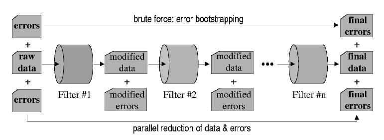
Figure 1: Classic reduction procedure.

0.2 The Classic Reduction Procedure

0.2.1 Three methods to quantify random errors

In a classic view (see Figure 1), a typical data reduction pipeline can be considered as a collection of filters, each of which transforms input images into new output images, after performing some kind of arithmetic manipulation and making use of additional measurements and calibration frames when required. Under this picture, three different approaches can in principle be employed to determine random errors in completely reduced images:

i) Comparison of independent repeated measurements. This is one of the simplest and most straightforward ways to estimate errors, since, in practice, errors are not computed nor handled through the reduction procedure. The only requirement is the availability of a non too small number of independent measurements. Although as such can be considered even the flux collected by each independent pixel in a detector (for example when determining the sky flux error in direct imaging), in most cases this method requires the comparison of different frames. For that reason, and given that for many purposes it may constitute an extremely expensive method in terms of observing time, its applicability on a general situation seems rather unlikely.

ii) First principles and brute force: error bootstrapping. Making use of the knowledge concerning how photo-electrons are generated (expected statistical distribution of photon arrival into each pixel, detector gain and read-out noise), it is possible to generate an error image associated to each raw-data frame. By means of error bootstrapping via Monte Carlo simulations, new instances of the initial raw-data frame are simulated and can be completely reduced as if they were real observations. The comparison of the measurements performed over the whole set of reduced simulated observations provides then a good estimation of the final errors. However, and although this method overcome the problem of wasting observing time, it can also be terribly expensive, but now in terms of computing time.

iii) First principles and elegance: parallel reduction of error and data frames. Instead of wasting either observing or computing time, it is also possible to feed the data reduction pipeline with both, the original raw-data frame and its associated error frame (computed from first principles), and proceed only once throughout the whole reduction process. In this case every single arithmetic manipulation performed over the data image must be translated, using the law of propagation of errors, into parallel manipulations of the error image. Unfortunately, typical astronomical data reduction packages (e.g. Iraf, Midas, etc.) do not consider random error propagation as a default operation and, thus, some kind of additional programming is unavoidable.

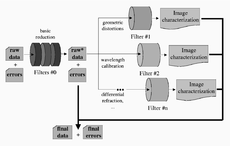
Figure 2: Modified reduction procedure.

0.2.2 Error correlation — A real problem

Although each of the three methods described above is suitable of being employed in different circumstances, the third approach is undoubtedly the one that, in practice, can be used in a more general situation. In fact, once the appropriate data reduction tool is available, the parallel reduction of data and error frames is the only way to proceed when observing or computing time demands are prohibitively high. However, due to the unavoidable fact that the information collected by detectors is physically sampled in pixels, this approach collides with a major problem: errors start to be correlated as soon as one introduces image manipulations involving rebinning or non-integer pixel shifts of data. A naive use of the analysis tools would neglect the effect of covariance terms, leading to dangerously underestimated final random errors. Actually, this is likely the most common situation since, initially, the classic reduction operates as a black box, unless specially modified for the contrary. Unfortunately, as soon as one accumulates a few reduction steps involving increment of correlation between adjacent pixels (e.g. image rectification when correcting for geometric distortions, wavelength calibration into a linear scale, etc.), the number of covariance terms starts to increase too rapidly to make it feasible the possibility of stacking up and propagate all the new coefficients for every single pixel of an image.

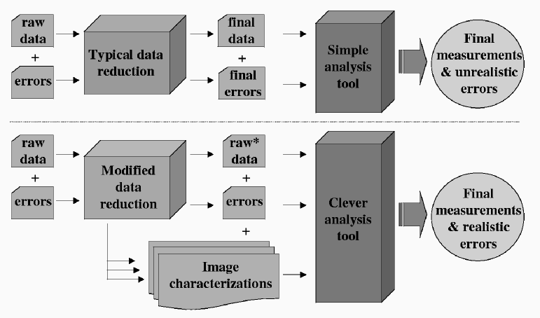
Figure 3: Comparison between classic (upper panel) and modified (lower panel) reduction procedures.

0.3 The Modified Reduction Procedure

0.3.1 Image Characterization

Obviously, the problem can be circumvented if one prevents its emergence, i.e. if one does not allow the data reduction process to introduce correlation into neighboring pixels before the final analysis. In other words, if all the reduction steps that lead to error correlation are performed in a single step during the measurement of the image properties with a scientific meaning for the astronomer, there are no previous covariance terms to be concerned with. Whether this is actually possible or not may depend on the type of reduction steps under consideration. In any case, a change in the philosophy of the classic reduction procedure can greatly help in alleviating the problem. The core of this change consists in considering the reductions steps that originate pixel correlation as filters that do not necessarily take input images and generate new versions of them after applying some kind of arithmetic manipulation, but as filters that properly characterize the image properties, without modifying those input images.

More precisely, the reduction steps can be segregated in two groups (see Figure 2): a) simple steps, which do not require data rebinning nor non-integer pixel shifts of data; and b) complex steps, those suitable of introducing error correlation between adjacent pixels. The former may be operated like in a classic reductions, since their application do not introduce covariance terms. However, the complex steps are only allowed to determine the required image properties that one would need to actually perform the correction. For the more common situations, this characterizations may be simple polynomials (in order to model geometric distortions, non-linear wavelength calibration scales, differential refraction dependence with wavelength, etc.). Under this view, the end product of the modified reduction procedure is constituted by a slightly modified version of the raw data frames (after quite simple arithmetic manipulations) and by an associated collection of image characterizations.

0.3.2 Modus Operandi

Clearly, at any moment it is possible to combine the result of the partial reduction after all the linkable simple steps, with the information achieved through all the characterizations derived from the complex steps, to obtain the same result than in a classic data reduction (thick line in Fig. 2). However, instead of trying to obtain completely reduced images ready for starting the analysis work, one can directly feed a clever analysis tool with the end products of the modified reduction procedure (see Figure 3). Obviously, this clever analysis tool has to perform its task taking into account that some reductions steps have not been performed. For instance, if one considers the study of a 2D spectroscopic image, the analysis tool should use the information concerning geometric distortions, wavelength calibration scale, differential refraction, etc., to obtain, for example, an equivalent width through the measurement in the partially reduced (uncorrected for geometric distortions, wavelength calibration, etc.) image. To accomplish this task, it is necessary to manipulate the data using a new and distorted system of coordinates that must override the orthogonal coordinate system defined by the physical pixels. It is in this step where the final error of the equivalent width should be obtained. It is important to highlight that, in this situation, such error estimation should not be a complex task, since the analysis tool is supposed to be handling uncorrelated pixels.

The described reduction philosophy will be incorporated into the pipeline data reduction for ELMER (http://www.gtc.iac.es/instrumentation/elmer_s.asp) and EMIR (http://www.ucm.es/info/emir).