A New Method for ISOCAM Data Reduction – II. Mid-Infrared Extragalactic Source Counts in the Southern ELAIS Field

Abstract

We present the 15 $\mu$m extragalactic source counts from the Final Analysis Catalogue of the European Large Area ISO Survey southern hemisphere field S1, extracted using the Lari method. The large number of extragalactic sources ($\sim 350$) detected over this area between about 0.5 and 100 mJy guarantee a high statistical significance of the source counts in the previously poorly covered flux density range between IRAS and the Deep ISOCAM Surveys. The bright counts in S1 ($S_{15~{}\mu m}{{}_{>}\atop{}^{\sim}}2$ mJy) are significantly lower than other published ISOCAM counts in the same flux range and are consistent with a flat, Euclidean slope, suggesting the dominance of a non-evolving population. In contrast, at fainter fluxes ($S_{15~{}\mu m}{{}_{<}\atop{}^{\sim}}2$ mJy) our counts show a strong departure from no evolution models, with a very steep super-Euclidean slope down to our flux limit ($\sim$0.5 mJy). Strong luminosity and density evolution of the order of, respectively, $L\propto(1+z)^{3.0}$ and $\rho\propto(1+z)^{3.5}$ is needed at least for the population of star-forming galaxies in order to fit the counts and the redshift distributions observed at different fluxes. A luminosity break around 10${}^{10.8}~{}L_{\odot}$ must be introduced in the local luminosity function of starburst galaxies in order to reproduce our sharp increase of the counts below 2 mJy and the redshift distributions observed for 15 $\mu$m sources at different flux levels. The contribution of the strongly evolving starburst population (down to 50 $\mu$Jy) to the 15 $\mu$m cosmic background is estimated to be $\sim$2.2 nW m^-2 sr^-1, which corresponds to $\sim$67% of the total mid-infrared background estimate.

1 Introduction

Deep galaxy counts are a key instrument for the study of galaxy evolution and can provide strong constraints to theoretical models. In fact, the departure of source counts from Euclidean predictions depends on the intrinsic evolution of galaxies and their redshift distribution. In the past few years several deep observations in different wave-bands have provided a significant advance in our knowledge of galaxy formation and evolution. Optical surveys found a strong evolution of the population of blue galaxies as a function of redshift to $z\sim 1$ (Lilly et al. 1996; Metcalfe et al. 1995), while Mid- and Far-Infrared deep surveys (Elbaz et al. 1999a,b, 2000; Dole et al. 1999), together with the detection of a substantial diffuse cosmic Infrared Background in the 300 $\mu$m - 1 mm range (Puget et al. 1996; Hauser et al. 1998; Fixsen et al. 1998; Lagache et al. 1999) implied a strong evolution also for galaxies emitting in the infrared. In fact, the Mid/Far-IR extragalactic background is at least as large as the UV/optical/NIR background, thus implying a stronger contribution of obscured star formation at redshifts larger than those observed by IRAS.

IRAS has sampled the local Universe ($z<0.2$) in the Mid/Far-IR band, discovering Luminous Infrared Galaxies (LIGs: $L>10^{11}L_{\odot}$) which radiate most of their light in the infrared band. Although LIGs are the most luminous starburst galaxies ever detected, they are relatively rare in the local Universe, thus making up only a small fraction of the total energy output from galaxies (Soifer & Negeubauer 1991). However, different analyses of the IRAS extragalactic source counts by Hacking, Houck and Condon (1987), Lonsdale & Hacking (1989), Saunders et al. (1990) and Kim and Sanders (1998) have shown some evidence for strong evolution at low flux density levels for ULIGs (Ultra-LIGs: $L_{Bol}\simeq L_{IR}>10^{12}L_{\odot}$). Due to the small redshift range sampled by IRAS, these results can only be indicative, though the suggestion that ULIGs might have played a stronger role in the past is supported by the detection of the strong infrared background.
With a thousand times better sensitivity and sixty times better resolution than IRAS, ISOCAM instrument (Cesarsky et al. 1996) on board of the Infrared Space Observatory (ISO; Kessler et al. 1996) has provided Deep and Ultra-Deep mid-infrared extragalactic surveys (mainly with the LW3 filter: 12 – 18 $\mu$m), unveiling most of the star-formation in the Universe to $z=1$. The source counts derived from these Deep/Ultra-Deep surveys (covering the flux density range 0.05 – 4 mJy) strongly diverge from no-evolution models at fluxes fainter than about 1 mJy, with an increasing difference that reaches a factor of 10 around the faintest limits (0.05 – 0.1 mJy; Elbaz et al. 1999a,b). The faint mid-infrared sources detected in the Deep/Ultra-Deep ISOCAM surveys have been identified mainly with galaxies at $z\simeq 0.7$ and show LIG-like luminosities (Aussel et al. 1999b; Elbaz et al. 1999a,b; Flores et al. 1999).

Although the Deep/Ultra-Deep ISOCAM Surveys have produced crucial results on galaxy evolution in the infrared, having identified most of the galaxies producing the mid-infrared background, there is a large gap in the flux density sampled by these surveys and by the IRAS Surveys. In particular, the flux density range 4 – 200 mJy is essentially uncovered in the Mid/Far–infrared and only a few sources have been detected by the Deep ISOCAM Surveys in the important flux range 1–4 mJy, where most of the existing evolutionary models (i.e. Franceschini et al. 2001; Xu 2000; Chary & Elbaz 2001; Rowan-Robinson 2001) predict a substantial change in the relative contribution of a local non-evolving and a more distant evolving population. This scarcity of data in this flux interval reflects also in a poor knowledge of the local luminosity function for starburst galaxies and a corresponding uncertainty in the evolutionary properties of the different classes of infrared extragalactic objects.

The European Large Area ISO Survey (ELAIS; Oliver et al. 2000) is the largest survey conducted with the Infrared Space Observatory (ISO) and provides a link between the IRAS survey and the Deep/Ultra-Deep ISOCAM surveys. ELAIS is a collaboration between 20 European institutes which involves a deep, wide-angle survey at high galactic latitudes, at wavelengths of 6.7 $\mu$m (LW2), 15 $\mu$m (LW3), 90 $\mu$m (C100) and 175 $\mu$m (C200) with ISO. In particular, the 15 $\mu$m survey covers a total area of $\sim$ 12 deg², divided into 4 main fields and several smaller areas. One of the main fields, S1, is located in the southern hemisphere. The whole S1 area has been surveyed in the radio (at 1.4 GHz, Gruppioni et al. 1999), in several optical bands (La Franca et al. 2002, in preparation) and in the hard X-ray with BeppoSAX (Alexander et al. 2001). Moreover, spectroscopic information and redshifts are available for a large number of sources (Gruppioni et al. 2001; La Franca, Gruppioni, Matute et al. 2002, in preparation).

We have reduced the 15$\mu$m data in S1 using a new ISOCAM data reduction technique (LARI technique) especially developed for the detection of faint sources, obtaining a catalogue (complete at the 5$\sigma$ level) of 462 sources in the flux density range 0.45 – 150 mJy. Details about the data reduction technique and the source catalogue have been presented in Lari et al. 2001 (hereafter Paper I). Here we present the source counts at 15 $\mu$m derived from that catalogue. The paper is structured as follows. In section 2 we give a brief description of the 15 $\mu$m ELAIS survey in S1. In section 3 we present the completeness and reliability of our sample at different flux levels. In section 4 we present the sample used to derive the source counts, which are shown in section 5. Finally, in sections 6 and 7 we discuss our results and their implications and present our conclusions.

Throughout this paper we will assume $H_{0}=50$ km s^-1 Mpc^-1, $\Omega_{m}=0.3$ and $\Omega_{\Lambda}=0.7$.

2 Description of the ELAIS S1 Survey

The ELAIS survey at 15 $\mu$m, performed in raster mode with the ISOCAM instrument on board of ISO, covers a total area of $\sim$ 12 deg² divided into 4 main fields and several smaller areas. The main field located in the southern hemisphere (S1) is centered at $\alpha$(2000) = 00^h 34^m 44.4^s, $\delta$(2000) = $-43^{\circ}$ 28^′ 12^′′ and covers an area of $2^{\circ}\times 2^{\circ}$. The 15 $\mu$m survey performed in S1 with the ISOCAM instrument consists of 9 different rasters. Each raster covers an area of $\sim 43.5^{\prime}\times 42^{\prime}$; eight of them have been observed once, while one, S1$\_$5, was observed three times.

The 15 $\mu$m data have been reduced and analyzed using the LARI technique, described in detail in Paper I. With this data reduction method, we have obtained a sample of 462 sources with signal-to-noise ratio $\geq 5$ in the flux range 0.45 – 150 mJy. The fainter sources have been detected in the central raster of S1 (S1$\_5$), whose image has been obtained by combining three single observations centered on the same position. The source catalogue in S1 and the relative parameter errors have been presented and discussed in Paper I, together with the detection rates at different flux densities derived with simulations.

The detection rates given in Paper I cannot be directly translated to completeness of the real catalogue, because our simulations were performed at discrete flux values rather than following a continuous flux distribution. However, the results presented in Paper I can be used to obtain the completeness of the catalogue and the source counts corrections, as discussed in the next section.

3 Completeness and Reliability

3.1 Brief Summary of the Results and Definitions from Paper I

Before describing in detail the method used to derive the completeness of our source counts, it is useful to summarize the more relevant results and definitions of Paper I. The simulations performed in the S1 field provided not only the completeness of our detections at different flux levels, but also the internal calibration of the source photometry and the distribution of the ratio between the measured and the theoretical peak fluxes (crucial for the computations described in next section).
Here we give some relevant definitions and relations:

• $f_{s}$: is the peak flux measured on maps for both real and simulated sources. Its value depends both on data reduction method and on ELAIS observing strategy $+$ ISOCAM instrumental effects;

• $f_{0}$: is the ‘theoretical’ peak flux measured on simulated maps containing neither glitches or noise. Its value depends only on ELAIS observing strategy $+$ ISOCAM instrumental effects;

• $q\equiv f_{s}/f_{0}$;

• $q_{med}$: is the peak of the $f_{s}/f_{0}$ distribution (also called systematic flux bias) and is 0.78 $\pm$ 0.03 in S1 and 0.82 $\pm$ 0.03 in S1$\_5$. These values are used to correct the measured flux densities;

• flux density determination:

  $$s=\left(\frac{f_{s}}{f_{0}}\times s_{0}\right)/q_{med}$$ (1)

  where for simulations $s_{0}$ is the injected total flux, while for real data $s_{0}$ is derived through successive iterations starting from a rough estimated value:

  $$s_{0}=f_{s}/\left<f_{s}/s_{0}\right>_{sim}$$ (2)

  where $\left<f_{s}/s_{0}\right>_{sim}=0.132$ is the average value resulting from simulations.
  We can consider $s$ as the measured flux density and $s_{0}$ as the ‘true’ flux density of a source;

• the photometric accuracy of our data reduction of the S1 area has been tested using the stars of the field and following the relation calibrated on IRAS data by Aussel & Alexander (2001) to predict the fluxes of stars. By a comparison between the predicted fluxes and the ones derived from our analysis, we have obtained a very good agreement and a relative flux scale of 1.096 $\pm$ 0.044 (i.e. our fluxes have to be multiplied by 1.096 to be put on the same scale as IRAS fluxes).

3.2 The g Function

As described in Paper I and mentioned in the previous section, with simulations in S1 we have derived the distribution of measured ($f_{s}$) to theoretical ($f_{0}$) peak flux ratio. This distribution is crucial in deriving the completeness of the catalogue and the internal flux calibration. To this purpose, we have considered the $f_{s}/f_{0}$ distribution as a model function, hereafter called $g~{}function$. The $g$ distribution function, obtained for simulated sources, is a combination of an intrinsic $g~{}function$ (referred as $g_{0}$) plus a term due to noise. As a rough estimate of $g_{0}$ in Paper I we considered the measured $g$ distribution obtained for 3 mJy simulated sources ($g_{0}\_{{}_{3}}$). Because 3 mJy is a relatively high flux density (it is the highest flux injected in our simulations), the $g_{0}\_{{}_{3}}$ distribution is almost unbiased by detection incompleteness, and we can consider it to be a good approximation of the intrinsic one. However, using the same simulation, we have obtained a more refined estimate of the intrinsic $g_{0}$ function correcting the observed $f_{s}/f_{0}$ distribution for the low level of detection incompleteness still present at this flux. Our procedure was the following:
each detected source $i$ has a $q_{i}=f_{s}(i)/f_{0}(i)$ value. On a different position $j$, assuming that the $f_{s}(i)/f_{0}(i)$ value is not depending on position, the peak flux would be measured with a value $f_{s,i}(j)=q_{i}\times f_{0}(j)$ and would be detected only if $f_{s,i}(j)$ were greater than 5 times the local noise ($\sigma(j)$). If $N_{i}$ is the number of possible detections in all the different $j$ positions of the simulations, the weight to be assigned to the $i^{th}$ source is $1/N_{i}$. Finally, the estimate of the intrinsic $g_{0}$ function in a given interval of $q$ is obtained by summing the weights of all the detected sources with a $q$ value in the same interval. By construction, the integral of $g_{0}$ over the entire range of $q$ is one.

Once obtained the $g_{0}$ distribution, the general $g$ distribution can be derived by convolving $g_{0}$ with the distribution of noise, here assumed to be Gaussian. This is possible in the approximation that the measured peak flux $f_{s}$ is the sum of a “true” value, $f_{s}^{t}$, and a stochastic term, $\chi$, due to noise, so that the $q$ ($\equiv$ $f_{s}$/$f_{0}$) measured value is:

$$q=\frac{f_{s}}{f_{0}}=\frac{f_{s}^{t}}{f_{0}}+\frac{\chi}{f_{0}}$$ (3)

with the $\chi$ term following a Gaussian distribution with average equal to zero and dispersion equal to the rms noise value, $\sigma$. Following this formalism, then the $g$ distribution, expressed as a function of $f_{s}/f_{0}$ and $f_{0}/\sigma$, is obtained by just convolving $g_{0}$ with the noise distribution, integrating over the possible values of the variable $\chi$:

$$g(\frac{f_{s}}{f_{0}},\frac{f_{0}}{\sigma})=\sqrt{\frac{1}{2\pi}}\frac{1}{\sigma}\int{g_{0}(\frac{f_{s}}{f_{0}}-\frac{\chi}{f_{0}})}\cdot e^{-\frac{\chi^{2}}{2\sigma^{2}}}d\chi$$ (4)

Figure 1: Predicted distributions of the ratio between the measured and the theoretical peak flux, $f_{s}/f_{0}$ (also $g~{}function$), in presence of a rms noise of 26 $\mu$Jy/pixel. These distributions, obtained from simulations, are shown for three different average values of $f_{0}$ corresponding to different input fluxes. The solid histogram shows the intrinsic $g_{0}$ distribution (see text)

In figure 1 we show the intrinsic $g_{0}$ distribution computed as above (solid histogram) and the predicted distributions of the ratio $f_{s}/f_{0}$ in presence of a $\sigma$ of 26 $\mu$Jy/pixel (typical of our data) for three different values of $f_{0}$, corresponding to different mean values of $f_{0}$ for different total input fluxes. As we can notice, the presence of noise broadens the flux distributions and this effect becomes stronger towards fainter fluxes (as shown also in figure 7 of Paper I).

If we assume that the g function reflects all the multiplicative and additive error components due to the data reduction, we can use this function to predict the distribution of the detection rate for both simulated and real sources, as described in the next subsection.

3.3 Completeness

First we have computed the incompleteness introduced by our data reduction method, represented by the loss of sources not accounted for by our model. In fact, sources can be missed by our method if interpreted as background transients. The incompleteness of our method is obtained from simulations by computing the ratio between the number of detections and the number of expected sources in different peak flux intervals ($[f_{0}-df_{0},f_{0}+df_{0}]$). The number of expected sources is derived by summing together the predicted detection contributions ($I_{i}(f_{0})=\int_{5\sigma/f_{0}}^{\infty}{g(q,f_{0})dq}$) of all the sources $i$ with peak flux $f_{0i}$ belonging to the same interval:

$$N_{exp}(f_{0})=\sum_{f_{0i}\in[f_{0}{\pm}df_{0}]}{I_{i}(f_{0})}$$ (5)

Figure 2: Completeness function of Lari method as function of the theoretical peak flux for S1 ($top$) and S1$\_5$ ($bottom$). The dashed lines give an estimate of the lower and upper envelopes of the completeness function.

In figure 2 the resulting function describing the incompleteness of our method is plotted as a function of $f_{0}$, together with its lower and upper envelopes, for S1 ($top$ panel) and S1$\_5$ ($bottom$ panel).

To obtain the global correction to be applied to our source counts, we need to consider also the areal coverage of our survey (i.e. the fraction of the survey area where a source of peak flux $f_{s}$ can be detected: $f_{s}\geq 5\sigma$) and the fact that real sources do not follow a discrete flux distribution as our simulated sources. To account for the latter effect, we have assumed a certain shape to describe the real source counts observed in the sky. According to the published counts at 15$\mu$m (e.g. Elbaz et al. 1999$a$), we have assumed two power laws between 0.4 and 150 mJy:

$$\frac{d{\cal N}}{ds}(s)\propto\left\{\begin{array}[]{ll}S^{-\alpha_{1}}&\mbox{if $S>2$ mJy}\\ S^{-\alpha_{2}}&\mbox{if $S<2$ mJy}\end{array}\right.$$ (6)

with $\alpha_{1}$=2.3 and $\alpha_{2}$=3.0 as first estimate values.
By weighting the above ’theoretical’ counts per unit of area by the $g~{}function$ convolved with the areal coverage function, and with the function describing the completeness of our method, we have computed the counts predicted in our Survey. Being $dN(s)=dN(s)/ds\cdot ds$ the number of sources detected in the flux density bin $ds$, $d{\cal N}(s_{0})=d{\cal N}(s_{0})/ds_{0}\cdot ds_{0}$ the theoretical number of sources detected in the ‘true’ flux density bin $ds_{0}$ and $ds_{0}/ds=q_{med}/q$ (from equation 1), we have:

$$\frac{dN}{ds}(s)=\left<\int_{0}^{\infty}dq~{}\left[g_{A}(q,f_{0}(s,q))\cdot C(f_{0}(s,q))\cdot\frac{d{\cal N}}{ds_{0}}(s_{0})\cdot\frac{ds_{0}}{ds}\right]\right>$$ (7)

$$=\left<\int_{0}^{\infty}dq~{}\left[g_{A}(q,f_{0}(s,q))\cdot C(f_{0}(s,q))\cdot\frac{d{\cal N}}{ds_{0}}(s_{0})\cdot\frac{q_{med}}{q}\right]\right>$$

where $g_{A}$ is the convolution of the $g~{}function$ with the areal coverage function and $C$ is the completeness function shown in figure 2. The averaging is performed over all the predicted peak flux values $f_{0}$ and with a random sampling of source positions in the survey. These expected source counts thus take into account the effects produced by the specific observational parameters of the ELAIS 15 $\mu$m survey and by our data reduction method. By putting $d{\cal N}(s_{0})/ds_{0}$ in the form given by equation 6 into equation 7, and changing $s_{0}$ to $s\cdot q_{med}/q$ (from equation 1), we obtain the source counts predicted for our survey, $dN(s)/ds$. The ratio between these counts and the theoretical source counts, $d{\cal N}(s_{0})/ds_{0}$, gives the global correction (including incompleteness and areal coverage) to be applied to our measured source counts. The inverse of the global correction (effective area) is reported in figure 3 for both $S1$ ($top$ panel) and $S1\_5$ ($bottom$ panel) surveys. Since our source counts corrected for incompleteness were significantly different from the original model counts (especially the power law at faint flux densities), we have iterated this procedure by adjusting the power laws parameters until convergence is achieved. The final estimate of the model counts $d{\cal N}(s)/ds$ is obtained for $\alpha_{1}$=2.3 and $\alpha_{2}$=3.6.

Figure 3: Effective area versus total flux density for the 15 $\mu$m catalogues in S1 main area ($top$) and S1$\_5$ ($bottom$).

4 The Data Sample Used for the Source Counts

The catalogue used to derive the source counts is not exactly the catalogue published in Paper I, but contains some differences, as described in this section.

First, we have conservatively decided to exclude from the source list used for counts 35 sources detected in S1, all with flux density $<1.5$ mJy, resulting “dubious” at a visual inspection of their pixel history. These sources, detected above the 5$\sigma$ threshold on the maps obtained through a combination of several images, are too faint to be distinguished from noise on the single pixel histories without uncertainty. Moreover, an additional factor which strengthened our doubts about the reliability of these sources is their very low optical identification rate. In fact, while for the entire catalogue (minus the 35 “dubious” sources) the optical identification rate (within a circle of 4 arcsec radius) on the DSS2 images for sources fainter than 1.5 mJy is 60%, for the 35 “dubious” sources it is only 14%, with a chance detection rate of about 10%.

Second, before computing the source counts we have applied three small further corrections to the flux densities presented in the catalogue of Paper I:

• We have applied the calibration factor of 1.096 derived from the comparison with stars in order to put our fluxes on the same scale as IRAS fluxes (see section 3.1 and section 7 in Paper I).

• We have corrected for the average underestimate of the true flux introduced by positional errors of the auto-simulated peak flux $f_{0}$ (see section 6 in Paper I); Since $f_{0}$ is computed on the measured positions and not on the ‘true’ ones, the measured flux is on average underestimated. This underestimate is flux dependent, due to the flux dependence of positional uncertainties. In figure 4 the corrections to be applied to the source flux densities due to this effect are reported as a function of signal to noise for both $S1$ (solid line) and $S1\_5$ (dashed line).

• In $S1\_5$ only we have corrected for the additional loss of flux due to the combination of the three rasters. To estimate this correction factor, for each source found in the combined $S1\_5$ map we have measured the flux in the three separate rasters and compared their average with the flux measured on the combined map. The mean ratio between the combined and the averaged single fluxes, considered as the correction factor, is $R=0.96\pm 0.01$.

Figure 4: Correction factors as function of signal to noise to be applied to the $S1$ ($solid$) and $S1\_5$ ($dashed$) source flux density to account for flux loss caused by positional errors in the theoretical peak flux $f_{0}$.

In the following statistical analysis we have chosen not to eliminate the 20 repeated sources (those belonging to the overlapping regions of two different rasters), but to consider them as different sources. The reason of this choice is that the detectability and completeness analysis, and consequently the correction factors to be applied to our data, have been performed on the single raster areas. This can explain why the effective area of S1 (see figure 3) corresponding to bright fluxes (= 8 times the area of one raster) is larger than the area of sky effectively covered by the S1 rasters. The sum of the effective areas shown in figure 3 is about 4.6 square degrees, while the S1 $+$ S1$\_5$ survey covers an area of 4 square degrees (about 15% of the area is covered by at least two rasters).

Finally, to compute the extragalactic source counts, we have excluded from our lists all the sources with a stellar counterpart brighter than $J=16$ in the Guide Star Catalogue II and with an evident stellar appearance (i.e. point-like with spikes) on the DSS2 images. We have chosen not to exclude any stellar identification fainter than $B_{J}=16$ found in the GSC-II (which is complete to $B_{J}=19.5$), because the reddest faint stars in our sample have estimated $B_{J}$ magnitude of the order of 15 (Aussel and Alexander 2001), and at fainter magnitudes the elimination from the sample of stellar-like objects might cause the elimination of AGN instead of stars. In fact, at $B_{J}{{}_{>}\atop{}^{\sim}}16$ the identifications with point-like objects are expected to be dominated by AGN.

Figure 5: Magnitude distribution of our stellar identifications (line-filled histogram) to $B_{J}=16$, compared to the magnitude distribution of all the GSC-II stars in the S1 area (empty histogram).

Figure 6: ISO-optical separation distribution for the stellar identifications in S1.

In the end, we have identified with stars, and subtracted from our list, 82 sources in S1 and 20 in S1$\_5$ (in total 102 stars, 87 of which are different), thus leaving a total of 325 extragalactic sources in S1+S1$\_5$ (320 different). The $B_{J}$ magnitude (from GSC-II) distribution of these stars is reported in figure 5 (filled histogram), where also the magnitude distribution of all the GSC-II stars in the S1 area is reported (to $B_{J}=16$). The maximum separation we find between ISO sources and star positions for our stellar identifications is ${{}_{<}\atop{}^{\sim}}4$ arcsec, as shown in figure 6. Given these positional differences and the surface density of stars, we estimate that less than one ISO/star association could be spurious (down to the considered magnitude limit $B_{j}=16$).
In figure 7 the fraction of stars in S1 is plotted as a function of flux density. At $S_{15~{}\mu m}{{}_{>}\atop{}^{\sim}}50$ mJy all our sources are identified with stars and still at $S_{15~{}\mu m}\simeq 5$ the fraction of stars is $\geq 50$%. For this reason, an accurate star subtraction is very important before computing the extragalactic ISOCAM counts, even at relatively faint fluxes (1-2 mJy), where the fraction of stars is still of the order of 20%.

Figure 7: Ratio between stars and the total number of 15 $\mu$m sources as a function of flux density for our S1 sample.

In the end, the extragalactic sample used to compute the source counts is composed by 325 source, 320 of which are different.

5 Source Counts

Given the extent of the 15 $\mu$m survey in S1 and the significant depth reached in its central area, S1$\_$5, our source sample is optimally suited to study the ISOCAM source counts with a large statistics and over a broad flux range (0.5 - 100 mJy). Therefore, the combined sample of our S1(main area) + S1$\_$5 non-stellar sources with $S_{15\mu m}\geq 5\sigma$ has been used to construct the mid-infrared extragalactic source counts distribution.

We used the effective areas derived in section 3 (see figure 3), to obtain the extragalactic mid-infrared source counts from our 15 $\mu$m samples.

Table 1: The 15 $\mu$m Source Counts in S1 + S1$\_5$

		S1			S1$\_5$			S1$+$S1$\_5$
$S$	$\left<S\right>$	$n$	$A_{eff}$	$dn/dS$	$n$	$A_{eff}$	$dn/dS$	$n$	$dn/dS$	$dn/dS\cdot S^{2.5}$	$N(>S)$
(mJy)	(mJy)		(deg2)	(deg-2 mJy-1)		(deg2)	(deg-2 mJy-1)		(deg-2 mJy-1)	(deg-2 mJy1.5)	(deg-2)
0.50 – 0.80	0.63	6	0.02	$-$	19	0.13	1344 $\pm$ 539	19	1344 $\pm$ 539	428 $\pm$ 171	544 $\pm$ 163
0.63 – 1.01	0.80	34	0.21	$672\pm 157$	27	0.27	521 $\pm$ 113	61	645 $\pm$ 109	369 $\pm$  62	353 $\pm$  42
0.80 – 1.28	1.01	76	0.90	$380\pm 59~{}$	21	0.38	161 $\pm$  36	97	280 $\pm$  33	288 $\pm$  34	194 $\pm$  17
1.01 – 1.62	1.28	88	2.00	$127\pm 5~{}~{}$	19	0.48	81 $\pm$   19	107	116 $\pm$  12	215 $\pm$  22	108 $\pm$   8
1.28 – 2.05	1.62	77	2.94	$44~{}\pm 5~{}~{}$	19	0.54	51 $\pm$   12	96	45 $\pm$  5	152 $\pm$  16	59.6 $\pm$ 4.4
1.62 – 2.75	2.11	67	3.57	$18~{}\pm 2~{}~{}$	16	0.54	26 $\pm$   7	83	20 $\pm$  2	126 $\pm$  14	37.8 $\pm$ 3.1
2.05 – 3.69	2.75	50	3.85	$8.1\pm 1.2$	10	0.54	11 $\pm$   4	60	8.6 $\pm$ 1.1	108 $\pm$  14	24.7 $\pm$ 2.4
2.75 – 4.95	3.69	34	4.00	$3.9\pm 0.7$	4	0.54	3.3 $\pm$ 1.7	38	3.9 $\pm$ 0.6	101 $\pm$  16	15.8 $\pm$ 1.9
3.69 – 6.64	4.95	24	4.00	$2.0\pm 0.4$	2	0.54	1.2 $\pm$ 0.9	26	1.9 $\pm$ 0.4	105 $\pm$  21	10.6 $\pm$ 1.5
4.95 – 8.90	6.64	18	4.00	$1.1\pm 0.3$	1	0.54	0.5 $\pm$ 0.5	19	1.1 $\pm$ 0.2	120 $\pm$  28	7.3 $\pm$ 1.3
6.64 – 11.9	8.90	11	4.00	$0.5\pm 0.2$	0	0.54	0.0 $\pm$ 0.0	11	0.5 $\pm$ 0.1	109 $\pm$  33	4.9 $\pm$ 1.0
8.90 – 18.9	13.0	7	4.00	$0.2\pm 0.1$	1	0.54	0.2 $\pm$ 0.2	8	0.2 $\pm$ 0.1	106 $\pm$  38	3.1 $\pm$ 0.8
11.9 – 29.9	18.9	5	4.00	$0.07\pm 0.03$	2	0.54	0.2 $\pm$ 0.1	7	0.09 $\pm$ 0.03	133 $\pm$  50	2.2 $\pm$ 0.7
18.9 – 47.2	29.9	2	4.00	$0.02\pm 0.01$	1	0.54	0.1 $\pm$ 0.1	3	0.02 $\pm$ 0.01	113 $\pm$  65	1.1 $\pm$ 0.5
29.9 – 74.6	47.2	3	4.00	$0.02\pm 0.01$	0	0.54	0.0 $\pm$ 0.0	3	0.02 $\pm$ 0.01	225 $\pm$ 130	0.7 $\pm$ 0.4
47.2 – 118.0	74.6	2	4.00	$0.007\pm 0.005$	0	0.54	0.0 $\pm$ 0.0	2	0.006 $\pm$ 0.004	298 $\pm$ 211	0.4 $\pm$ 0.3

In Table 1 the 15 $\mu$m source counts in S1, S1$\_5$ and S1+S1$\_5$ areas are presented. We have first computed the counts for the two samples in S1 and S1$\_5$ separately, as reported in the first eight columns of Table 1, giving respectively the adopted flux density intervals, the average flux density in each interval (computed as the geometric mean of the two flux density limits), the observed number of sources, the effective area (figure 3$top$), the differential source counts and their associated errors in S1 and the observed number of sources, the effective area (figure 3 $bottom$) and the differential source counts with their errors in S1$\_5$. The differential source counts have been obtained by weighting each single source for its effective area rather than weighting the total number of sources in each flux density bin for the effective area corresponding to the reference flux density of that bin. The errors associated to the counts in each bin have been computed as $\sqrt{\Sigma_{i}(1/A_{eff}^{2}(S_{i}))}$, where the sum is for all the sources with flux density $S_{i}$ belonging to the bin and $A_{eff}(S_{i})$ is the effective area corresponding to that source flux. These errors take into account only the Poissonian term of the uncertainties associated to the source counts, for consistency with the other literature works. Especially at faint flux density, where the effective area (and consequently the correction factor) is a steep function of flux, the errors quoted in Table 1 should be considered as lower limits of the ‘true’ errors (including also the uncertainty in the effective area computation, shown as dashed curves in figure 3).
The counts computed for S1 and S1$\_5$ are consistent within the errors in most flux density intervals, the only exception being the 0.8 - 1.2 mJy flux bin, where the counts in S1 are larger than the ones in S1$\_5$ at a formal level of $\sim 2.3\sigma$. However, since the low flux density errors are somewhat underestimated, we can consider the source counts in S1 and S1$\_5$ consistent in all the common flux density intervals, over the whole range 0.5 - 100 mJy.
For this reason, we have also computed the source counts in the “combined” sample (S1$+$S1$\_5$), by considering all the sources as belonging to a unique sample: for each source the combined effective area is the sum of the effective areas in S1 and S1$\_5$ (whose values are reported in column 4 and 7 respectively). In the last four columns the total number of sources in each flux density bin, the differential source counts, the differential counts normalized to the Euclidean distribution (by multiplying by $\left<s\right>^{2.5}$) with their errors and the integral source counts (with errors) for the combined sample are reported. In the first flux density bin the counts for the combined sample coincide with the $S1\_5$ counts, since, due to their negligible effective area, we have not considered the $S1$ data.

Note that the flux bins are partially overlapping, therefore they are not statistically independent (they are alternately independent). The choice of partially overlapping flux density bins for our source counts representation is based on the need of a tight sampling of the region where the counts start diverging from no evolution models, in order to better determine the break point and the counts shape (with a larger statistics). As mentioned in the previous section, in computing the counts we have considered as two different sources those appearing in two different rasters (belonging to the border part of a raster, overlapping with an adjacent raster), by suitably weighting them for their detectability area in each raster. In fact, in deriving the areal coverage function we have considered the total area of each single raster, including the overlapping regions.

Figure 8: Differential source counts at 15 $\mu$m normalized to the Euclidean distribution ($N(S)\propto S^{-2.5}$). Data points (as shown also in the figure): A2390 (open diamonds), ISO HDF–N (open circles), ISO HDF–S (filled circles), Marano Firback (open squares), Marano Ultra-Deep (diagonal crosses), Marano Deep (asterisks), Lockman Deep (open triangles), Lockman Shallow (filled triangles), ELAIS S1 (filled stars). The dotted curves are the lower and upper envelopes of our counts due to the uncertainties in the completeness curve derivation, as shown in figure 3. The hatched area represents the range of possible expectations from no evolution models normalized to the IRAS 12 $\mu$m Local Luminosity Function (upper limit from Rush, Malkan & Spinoglio 1993; lower limit from Fang et al. 1998).

The 15 $\mu$m differential source counts of the combined ELAIS S1 and S1$\_5$ data, normalized to those expected in a Euclidean geometry by dividing by $S^{-2.5}$, are shown in figure 8 (filled stars). For comparison, source counts from other ISOCAM surveys (A2390 from Altieri et al. 1999; ISO HDF-N from Aussel et al. 1999a; ISO HDF-S, Marano Firback, Marano Ultra-Deep, Marano Deep, Lockman Deep, Lockman Shallow from Elbaz et al. 1999b; data kindly provided by D. Fadda, private communication) are also plotted. Our counts are lower than the Lockman Deep and Shallow ones. However, they appear consistent with the counts obtained in the Marano Deep Survey, at least in the common flux density range (0.5 – 2 mJy).

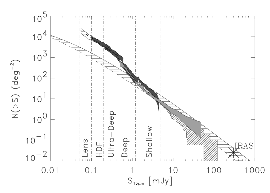
Figure 9: Integral source counts for extragalactic ISOCAM sources detected at 15 $\mu$m above a given flux $S$. The grey-shaded area shows the integral extragalactic counts with 68% confidence contours obtained from the ELAIS S1 Survey (this work). For comparison, the hatched and the black-shaded areas represent the counts with 68% confidence contours obtained respectively from the ELAIS Preliminary Analysis, normalizing downwards by a factor of 2 the fluxes of Serjeant et al. (2000), and from the ISOCAM Deep/Ultra-Deep Surveys (Elbaz et al. 1999b). The area filled with horizontal lines represents the range of possible expectations from no-evolution models normalized to the IRAS 12$\mu$m local luminosity function, as reported in figure 8. The fainter end of the IRAS 12$\mu$m source counts derived by Rush, Malkan and Spinoglio (1993), converted to 15 $\mu$m, is represented by the asterisk.

In figure 9 our integral extragalactic source counts are reported. The grey-shaded area shows the integral extragalactic counts with 68% confidence contours obtained from the ELAIS S1 + S1$\_5$ Survey. For comparison, the black-shaded area represents the counts with 68% confidence contours obtained from the ISOCAM Deep/Ultra-Deep Surveys (Elbaz et al. 1999b). The hatched area represents the integral counts of Serjeant et al. (2000) based on the Preliminary Analysis of the whole ELAIS Survey, with fluxes rescaled downward by an average factor of 2, as suggested by a recent calibration work (i.e. Väisänen et al. 2002). The area filled with horizontal lines represents the range of possible expectations from no-evolution models normalized to the IRAS 12$\mu$m local luminosity function. The asterisk represents the fainter end of the IRAS 12$\mu$m source counts derived by Rush, Malkan and Spinoglio (1993), opportunely converted to 15 $\mu$m.

Our data reduction allowed us to compute source counts down to fluxes $\sim$3 times fainter than the Preliminary Analysis (PA) of the ELAIS data (Serjeant et al. 2000). In the flux range common to the two samples we find that, after correcting downward the PA fluxes by a factor of 2, our source counts are in reasonably good agreement with the counts of Serjeant et al. (2000) above $\sim$2.5 mJy. However, the overall slope of the Serjeant et al. counts appears to be steeper than ours, with our counts being lower below 2.5 mJy and somewhat higher above 10 mJy. This is probably due the fact that a flux dependent calibration correction, rather than a constant correction, should be applied to the Serjeant et al. (2000) fluxes. In fact, there are hints (Babbedge and Rowan-Robinson 2002, in preparation) that the needed correction factor is $\sim$2.4 for the fainter PA fluxes and $\sim$1.75 for the brighter fluxes (the factor of 2 here adopted is an average value).

Our counts, though not deep enough to detect the fast convergence at flux densities fainter than 0.4 mJy shown by the Deep/Ultra-Deep ISOCAM counts, sample very well the flux density range where those counts start diverging from no evolution models. Indeed, we observe a remarkable change in the slope of our counts, showing a significant super-Euclidean slope from about 2 mJy to $\sim$0.45 mJy. Due to its large statistics, our Survey is at the moment best suited for determining both the exact flux density where the 15 $\mu$m extragalactic counts steepen and the count slope itself (before and after the steepening). A maximum likelihood fit to our extragalactic source counts with two power laws:

$$\frac{dN}{dS}\propto\left\{\begin{array}[]{ll}S^{-\alpha_{1}}&\mbox{if $S>S_{b}$}\\ S^{-\alpha_{2}}&\mbox{if $S<S_{b}$}\end{array}\right.$$ (8)

gives the following parameters: $\alpha_{1}=2.35\pm 0.05$, $\alpha_{2}=3.60\pm 0.05$, $S_{b}=$($2.15\pm 0.05$) mJy. Our best fit parameters suggest that the steepening of the integral counts starts around 2 mJy, then the counts keep a super-Euclidean slope down to the limits of our survey ($\sim$0.5 mJy).

6 Discussion

6.1 Comparison with Deep/Ultra-Deep ISOCAM Surveys Source Counts

The 15 $\mu$m extragalactic source counts derived from the southern ELAIS Survey cover over two decades in flux, from 0.5 up to 100 mJy, with a significant statistical sampling (325 objects). Due to the large flux density interval covered, the ELAIS counts bridge the gap existing between the IRAS counts and the ISOCAM Deep/Ultra-Deep counts. The ELAIS Survey was planned to be a shallow survey and to reach an optimistic limit of about 2 mJy. As shown in Paper I, with the Lari technique we were able to go much deeper than expected, detecting a significant number of sources even at sub-mJy levels. The strength of ELAIS counts is at fluxes brighter than $\sim$1 mJy, where they are highly statistically significant and complete. At fainter fluxes, though the S1 and S1$\_5$ counts are consistent over the whole flux range, the results are less strong due to the large incompleteness correction required by the S1 data and the small area covered by the more complete S1$\_5$ data. However, the results are consistent with the evolution scenario found by other ISOCAM surveys and are able to give general hints on the behaviour and evolution of infrared galaxies. In particular, ELAIS counts in the flux density range in common with ISOCAM Deep counts (0.5 – 4 mJy) diverge from no evolution models as well and steepen with a super-Euclidean slope (3.60 $\pm$ 0.05 for the differential form) up to the fainter limit. In particular, the flux density where our counts start diverging from no evolution predictions is (2.15 $\pm$ 0.05) mJy. Above this flux density, the ELAIS counts are consistent with no evolution, showing a slope (in differential form) of 2.35 $\pm$ 0.05. Although similar results have been found for the Deep ISOCAM Surveys, between 0.5 and $\sim$2 mJy our counts are somewhat steeper and on average lower than the others. However, the common flux range is sampled by three Deep Surveys only: Marano Deep, Lockman Deep and Lockman Shallow. The counts drawn from the Marano Deep Survey appear consistent with the ELAIS counts, while the counts obtained from both Lockman Deep and Shallow Surveys are less steep at faint fluxes (especially the Lockman Shallow ones) and higher than ours by about a factor of 2-3 around 2-3 mJy.

The reason for this discrepancy is still not completely understood. It could be due to different separate causes or to a combination of them. A possible reason might be attributed to different data reduction methods applied to different surveys. For example, our survey has been reduced with the Lari method (see Paper I), while the Marano and the Lockman Deep Surveys have been reduced with the PRETI method (Starck et al. 1999) and the Lockman Shallow Survey has been reduced with the triple beam switch method of IAS (Desért et al. 1999). We must note that the PRETI method was especially designed to account for all the spurious effects of ISOCAM data in a more complete way than the triple beam switch method. A comparison between these two methods performed in the HDF-N (Aussel et al. 1999a) has produced similar results, although not all the sources detected by one method were present in the list found by the other method. Moreover, flux densities derived for the common sources with the triple beam switch method were sistematically lower, by a factor of 0.82, than the PRETI fluxes. In fact, each method measures fluxes in a different way (i.e. auto-simulations for Lari, photometry aperture plus implicit colour correction for PRETI, fit with a fixed width Gaussian for the triple beam switch) and this might produce small differences in the photometry of the objects. However, if our fluxes were on the same scale as the PRETI ones, the assumption that the triple beam switch fluxes are 20% lower would furtherly increase the observed discrepancy between our counts and the Lockman Shallow counts. Viceversa, good agreement between Lockman Deep counts and our counts would be obtained if the Lockman Deep fluxes were systematically higher than ours by about 15% (see figure 10). The flux calibration of our catalogue, as described in detail in Paper I, has been tested using the stars in the field and resulted on the same flux scale of IRAS (relative flux scale of 1.096 $\pm$ 0.044), with photometric errors not larger than 10%.

Figure 10: Zoom of the normalized differential source counts at 15 $\mu$m. The symbols are the same as in figure 8: filled stars for ELAIS counts and open triangles for Lockman Deep counts. The upper Lockman points are the original counts, while the lower ones are the counts obtained with 15% lowered fluxes.

Another possible cause of the counts difference could be an incomplete star subtraction performed in the Lockman Surveys, whose brightest flux density bins (at 2-5 mJy) might contain between 20 and 50% of stars (as shown in section 5).

Finally, part of the observed discrepancy could also be due to cosmic variance affecting small area fields, like the Marano Deep Field (0.2 sq. deg.) and the Lockman Deep and Shallow Fields (respectively 0.14 and 0.54 sq. deg.).

6.2 Models and Interpretation

As already mentioned, at flux densities ${{}_{>}\atop{}^{\sim}}$ 1-2 mJy, the ELAIS counts are consistent with the expectation of models assuming no evolution for extragalactic sources, while they strongly depart from no evolution predictions at fainter fluxes. The almost flat differential counts (normalised to Euclidean) extending from the IRAS fluxes to 1-2 mJy, followed by the sudden upturn below, seem to require strong evolution for a single population rather than for the whole population of 15 $\mu$m galaxies.
Due to the uncertainties existing in our counts at faint fluxes, in this paper we do not pretend to construct an evolutionary model based on our result, however, in order to interpret our data and the evolution they seem to require, we have compared our counts with recent evolution models for mid-infrared galaxies found in literature. In particular, we have compared our counts with the models of Xu (2000) and Franceschini et al. (2001). Neither model is able to reproduce the sharp departure feature from no-evolution predictions, or the low ‘plateau’ between 1-2 and 100 mJy shown by our data. The Xu (2000) model is able to fit the Deep/Ultra-Deep ISOCAM counts by considering a rather extreme luminosity evolution (i.e. $L(z)=L(0)\times(1+z)^{4.5}$) for the whole infrared population. However, it largely over-predicts our counts above 0.8-1 mJy and its departure from no evolution predictions is far too smooth to reproduce the sharp upturn shown by our data around 2 mJy. The model predictions of Franceschini et al. (2001) are somewhat steeper than the Xu ones, but still overestimating and smoother than our counts, though considering a combination of luminosity and density evolution for star-forming galaxies only. The local luminosity functions (LLFs) on which these models are based are different: the one considered by Xu (2000) has been derived using the bivariate (15 $\mu$m vs. 60 $\mu$m luminosities) method, from an IRAS sample selected at 60 $\mu$m and observed by ISOCAM at 15 $\mu$m, while the one used by Franceschini et al. (2001) is an adapted combination of the 12 $\mu$m LLF from Fang et al. (1998) and the bivariate 15 - 60 $\mu$m, converted to 12 $\mu$m, from Xu et al. (1998). Franceschini et al. (2001) have also tried to disentangle the contributions of different populations. Due to its larger flexibility in allowing to play with the different populations and their evolutionary properties, we have based our analysis on the Franceschini et al. (2001) models, trying to find a good fit to our data by varying the LLF free parameters.
These models are able to reproduce the Deep/Ultra-Deep ISOCAM counts by considering different evolutionary properties for three different populations: non-evolving normal spirals, strongly evolving starburst plus Seyfert 2 galaxies and evolving AGN 1. The latter are assumed to evolve in luminosity as $L(z)=L(0)\times(1+z)^{3}$ up to $z=1.5$ and constant luminosity density at higher redshift. For the population of star-forming and Seyfert 2 galaxies, in a $H_{0}=50$ km s^-1 Mpc^-1, $\Omega_{m}=0.3$, $\Omega_{\Lambda}=0.7$ Universe, the best-fit to Deep/Ultra-Deep ISOCAM counts is found by Franceschini et al. (2001) by considering luminosity evolution $L(z)=L(0)\times(1+z)^{3.8}$ and density evolution $\rho(L[z],z)=\rho_{0}(L)\times(1+z)^{4}$ up to $z_{break}=0.8$, and no additional evolution at $z>z_{break}$.

Figure 11: Best fit model (re-adapted from Franceschini et al. 2001) to ELAIS S1 source counts. The dotted line corresponds to the expected counts for a population of non-evolving spirals. The short-dashed line is the modeled contribution of a population of strongly evolving starburst (plus Seyfert 2) galaxies, while the long-dashed line is the contribution of type I AGN. The solid line represents the expected total source counts.

We have not changed either the evolution (form and rate) for AGN 1, nor the evolutionary scheme for star-forming (plus Seyfert 2) galaxies. However, for the latter, we have varied the luminosity and density evolution rates (respectively $\alpha_{L}$ and $\alpha_{D}$ hereafter), $z_{break}$, and the LLF normalization. The crucial point is the star-forming galaxy LLF and in particular its shape at bright luminosities. In order to fit the sharp rise of our counts below 2 mJy, we have found essential to introduce a luminosity break ($L_{break}$) in the star-forming LLF, above which it quickly drops to zero. This is also strongly required by the redshift distribution for bright sources (above few mJy). In fact, without any luminosity break in the LLF, the redshift distribution predicted by the Franceschini et al. (2001) model for example for sources brighter than 5 mJy, shows a significant secondary peak around $z\sim 1$, in addition to a low redshift peak. This is not consistent with the redshifts measured for bright ELAIS sources ($S\geq 2$ mJy; Gruppioni et al. 2001; La Franca, Gruppioni, Matute et al. 2002, in preparation), which are all found to be at rather low redshifts ($z<0.3-0.4$).

We have taken into account the redshift distribution constraints when looking for the best fit to our observed source counts. In particular, we have asked the model results to roughly agree with the following observational evidences:

• absence of high redshift peak for bright ($\geq 2$ mJy) sources (Gruppioni et al. 2001; La Franca, Gruppioni, Matute et al. 2002, in preparation);

• majority of sources at moderate redshifts ($z<0.3-0.4$) even at fluxes $S\geq 0.8-1$ mJy, with a fraction of high $z$ sources not larger than 30 - 35% (Pozzi, Ciliegi, Gruppioni et al., 2002, in preparation);

• redshift distribution for Deep surveys ($S\geq 0.1-0.2$ mJy) showing a peak between $z=0.5$ and $z=1.2$ (HDF-North: Aussel et al. 1999b, Aussel et al. in preparation, as reported by Franceschini et al. 2001; CFRS 11415+52: Flores et al. 1999).

Figure 12: Redshift distributions predicted by our best fit model for 15 $\mu$m sources at different flux levels and in different areas. $Top$: $S\geq 2$ mJy, area = 4 deg² (S1); $middle$: $S\geq 1$ mJy, area = 4 deg² (S1); $bottom$: $S\geq 0.12$ mJy, area = $6\times 10^{-3}$ deg² (HDF-N). The latter is computed for the HDF-N area and to the same flux limit for a direct comparison with the redshift distribution observed in that field (Aussel et al. 2002, in preparation).

The best solution was found for $\alpha_{L}=3.0$, $\alpha_{D}=3.5$, $z_{break}=1.1$, a LLF of evolving starburst population 40% higher than the Franceschini one and $L_{break}=10^{10.8}L_{\odot}$. In figure 11 the fit to source counts obtained with the above parameters is shown, while the redshift distributions expected for our survey at $S_{15~{}\mu m}\geq$ 0.1, 1.0 and 2.0 mJy are plotted in figure 12. These distributions are in good agreement with the preliminary results of optical identification for the S1 sources on the DSS2. We find, in fact, that, while above 2 mJy most sources have an optical counterpart brighter than $R\simeq 21.5$ (92 % at $S_{15~{}\mu m}\geq 2$ mJy and 95% at $S_{15~{}\mu m}\geq 3$ mJy), between 1 and 2 mJy there is a quick drop in the identification fraction (it goes down to $\sim$70%), probably associated to a change in population (i.e. appearance of the high-$z$ excess number of sources in the redshift distribution). At $S_{15~{}\mu m}\geq 1$ mJy, the expected high-$z$ ($z\geq 0.6$) fraction of sources is $\sim$35%, in good agreement with the fraction of S1 sources to the same flux density without optical counterpart on the DSS2.

Our result shows that significant evolution is needed for at least a class of extragalactic objects, in order to explain the observed source counts below a few mJy. Above about 10 mJy the counts are dominated by a non-evolving population of normal spiral galaxies, while below this flux density a population of strongly evolving starburst galaxies shows up and, rapidly rising, starts dominating the counts. At fluxes ${{}_{<}\atop{}^{\sim}}3-5$ mJy, evolving starburst galaxies make up most of the observed counts, being responsible for the peak around 0.3-0.4 mJy revealed by the Deep and Ultra-Deep ISOCAM Surveys. The evolution required for this class of objects is lower than found by Franceschini et al. (2001): $\alpha_{L}$ is 3.0 instead of 3.8 and $\alpha_{D}$ is 3.5 instead of 4.0. However, a turnover at higher $z$ ($z_{break}=$ 1.1 instead of 0.8) is needed in order to reproduce both the sharp rise of our counts and the faint flux peak of the Deep ISOCAM Surveys counts. This value for $z_{break}$ is intermediate between 0.8 found by Franceschini et al. (2001) and 1.5 found by Xu (2000), though the latter obtains a reasonably good fit to the Deep/Ultra-Deep counts and to the redshift distribution of ISOCAM sources in the HDF-North (Aussel et al. 1999b), by considering pure luminosity evolution (with $\alpha_{L}=4.5$) for the whole 15 $\mu$m extragalactic population. However, the Xu (2000) model is not able to fit the new redshift distribution observed in the HDF-North with $>$ 90% complete spectroscopic identification, as derived by Aussel et al. (2002 in preparation) and reported by Franceschini et al. (2001).

We have obtained an estimate of the 15 $\mu$m CIRB flux by directly integrating the best-fit model counts down to $S_{15~{}\mu m}=50~{}\mu$Jy: 2.2 nW m^-2 sr^-1. This value is in good agreement with the computation done by Elbaz et al. (2001, as reported by Chary & Elbaz 2001), who finds a value of 2.4 $\pm$ 0.5 nW m^-2 sr^-1 by integrating the observed ISOCAM Deep/Ultra-Deep counts down to the same flux density limit. Our estimate of the 15 $\mu$m CIRB flux corresponds to about 67% of the total resolved CIRB at 15 $\mu$m derived by Biviano et al. (2000) as 3.3 $\pm$ 1.3 nW m^-2 sr^-1.

7 Conclusions

ISOCAM extragalactic source counts in the flux density range 0.5 – 100 mJy have been derived for the ELAIS 15 $\mu$m samples obtained in the southern hemisphere area with a new data reduction technique (see Paper I). Our counts sample very well the flux density region where Deep/Ultra-Deep ISOCAM counts start diverging from no evolution models. Indeed, we observe a significant change in slope from a value of $\sim$2.35 at fluxes higher than $S\simeq 2$ mJy to a very steep value ($\alpha\sim 3.60$) for fainter fluxes down to our flux limit ($S\simeq 0.5$ mJy).
This is in qualitative agreement with previous results, although the ELAIS counts show a somewhat steeper slope at faint fluxes than the other surveys ($\alpha\simeq 3.0$ between 0.4 and 4 mJy; Elbaz et al. 1999b). At the faintest limit of our survey ($S\sim 0.5-1.0$ mJy), where data from a number of other surveys exist, our counts agree with those obtained in the Marano Deep Survey and are somewhat lower than those obtained in other surveys. At brighter fluxes ($S{{}_{>}\atop{}^{\sim}}2-5$ mJy), where our data are highly complete and statistically significant (because of the large sampled area), our counts are significantly lower than the counts in the Lockman Deep and Shallow Surveys. The observed difference might be attributable to different reduction methods applied to different surveys, to not complete star subtractions and to cosmic variance that could affect small area surveys (i.e. Lockman Deep and Shallow, Marano Deep).

A good fit to our counts is obtained by re-adapting Franceschini et al. (2001) model and introducing a luminosity break in the local luminosity function of the evolving population. Our solution considers no evolution for normal spiral galaxies (dominating the counts at fluxes ${{}_{>}\atop{}^{\sim}}5-10$ mJy), a combination of luminosity and density evolution ($L(z)=L(0)\times(1+z)^{3.0}$ and $\rho(L[z],z)=\rho_{0}(L)\times(1+z)^{3.5}$) up to $z_{break}=1.1$ for starburst galaxies, with a break in their LLF at $L_{15~{}\mu m}=10^{10.8}L_{\odot}$, and luminosity evolution ($L(z)=L(0)\times(1+z)^{3.0}$ up to $z=1.5$) for type 1 AGN. Strongly evolving starburst galaxies rise quickly below $\sim 10$ mJy and start making up almost the totality of the observed counts at fluxes fainter than a few mJy. Our results are also in agreement with the observed redshift distributions at different flux levels (from 10 down to 0.1 mJy), predicting a rather local population ($z_{med}\simeq 0.2$) of star-forming galaxies down to $\sim$1.5 mJy and a rapid rise of a high-$z$ ($z_{med}\simeq 1$) excess of objects at fainter flux densities. This high-$z$ population totally dominates below $\sim 0.5$ mJy.

References

- [Alexander et al. 2001] Alexander D.M., La Franca F., Fiore F., Barcons, X., Ciliegi P., Danese L., Della Ceca R., Franceschini A., Gruppioni C., Matt G., Oliver S., Pompilio F., Wolter A., Efstathiou A., Perola G.C., Perri M., Rigopoulou D., Rowan-Robinson M. & Serjeant S., 2001, ApJ, 554, 18
- [Altieri et al. 1999] Altieri B., Metcalfe L. & Kneib J.P., 1999, A&A, 343, L65
- [Aussel and Alexander] Aussel H. & Alexander D.M., 2001, AAS, 198, 4910
- [Aussel et al. 1999a] Aussel H., Césarsky C.J., Elbaz D. & Starck J.-L., 1999a, A&A, 342, 313
- [Aussel et al. 1999b] Aussel H., Elbaz D., Césarsky C.J. & Starck J.-L., 1999b, The Universe as seen by ISO, P. Cox & M.F. Kessler, ESA Special Publication series (SP-427), p. 1023
- [Aussel et al. 2002] Aussel H. et al., 2002, in preparation
- [Babbedge and Rowan-Robinson 2002] Babbedge T. & Rowan-Robinson M., 2002, in preparation
- [Biviano et al. 2000] Biviano A., Metcalfe L., Altieri B., Leech K., Schulz B., Kessler M.F., McBreen B., Delaney M., Kneib J.-P., Soucail G., Okumura K., Elbaz D., and Aussel H., 2000, Clustering at High Redshift, A. Mazure, O. Le F vre and V. Le Brun, ASP Conference Series, vol. 200, p. 101 (astro-ph/9910314)
- [Cesarsky et al. 1996] Cesarsky C.J., Abergel A., Agnèsel P. et al., 1996, A&A, 315, L32
- [Chary and Elbaz 2001] Chary R. & Elbaz D., 2001, ApJ, 556, 562
- [Dole et al. 1999] Dole H., Lagache G., Puget J.-L. et al., 1999, The Universe as seen by ISO, P. Cox & M.F. Kessler, ESA Special Publication series (SP-427), p. 1031
- [Desert et al. 1999] Désert F.-X., Puget J.-L., Clements D.L., Pérault M., Abergel A., Bernard J.-P. & Cesarsky C.J., 1999, A&A, 342, 363
- [Elbaz et al. 1999a] Elbaz D., Aussel H., Césarsky C.J., Désert F.X., Fadda D., Franceschini A., Harwit M., Puget J.-L., & Starck J.-L., 1999a, The Universe as seen by ISO, P. Cox & M.F. Kessler, ESA Special Publication series (SP-427), p. 999
- [Elbaz et al. 1999b] Elbaz D., Césarsky C.J., Fadda D., Aussel H., Désert F.-X., Franceschini A., Flores H., Harwit M., Puget J.-L., Starck J.-L., Clements D.L., Danese L., Koo D. C. & Mandolesi R., 1999b, A&A, 351, L37
- [Elbaz 2000] Elbaz D., 2000, Building Galaxies: from the Primordial Universe to the Present, F. Hammer, T.X. Thuan, V. Cayatte, B. Guiderdoni, & J. Tran Thanh Van (Edition Frontieres), in press (astro-ph/9911050)
- [Elbaz et al. 2000] Elbaz D., Cesarsky C.J., Chanial D., Aussel H., Franceschini F., Fadda D., Chary L., 2002, ApJ, in press
- [Fixsen et al. 1998] Fixen D.J., Dwek E., Mather J.C., Bennett C.L. & Shafer R.A., 1998, ApJ, 508, 123
- [Fang et al. 1998] Fang F., Shupe D., Xu C. & Hacking P., 1998, ApJ, 500, 693
- [Flores et al. 1999] Flores H., Hammer F., Thuan T.X., Césarsky C., Desert F.X., Omont A., Lilly S.J., Eales S., Crampton D. & Le F vre O., 1999, ApJ, 517, 148
- [Franceschini et al. 1997] Franceschini A., Aussel H., Bressan A., Cesarsky C.J., Danese L., De Zotti G., Elbaz D., Granato G.L., Mazzei P., & Silva L., 1997, The Far Infrared ans Sub-Millimeter Universe, E. Wilson, ESA Special Publication Series (SP-401), p. 159
- [Franceschini et al. 2001] Franceschini A., Aussel H., Cesarsky C.J., Elbaz D. & Fadda D., 2001, A&A, 378,1
- [Gruppioni et al. 2001] Gruppioni C., Pozzi F., Ciliegi P., Mignoli M., La Franca F., Oliver S. & Rowan–Robinson M., 2001, The Far-Infrared and Sub-Millimeter Spectral Energy Distributions of Active and Starburst Galaxies, I. Van Bemmel, P. Barthel & B. Wilkes, New Astronomy Reviews series (Elsevier), in press
- [Gruppioni et al. 1999] Gruppioni C., Ciliegi P., Rowan-Robinson M., Cram L., Hopkins A., Cesarsky C., Danese L., Franceschini A., Genzel R., Lawrence A., Lemke D., McMahon R.G., Miley G., Oliver S., Puget J-L & Rocca-Volmerange B., 1999, MNRAS, 305, 297
- [Hacking et al. 1987] Hacking P.B., Houck J.R. & Condon J.J., 1987, ApJ, 316, 15
- [Hauser et al. 1998] Hauser M.G., Arendt R.G. & Kelsall T., 1998, ApJ, 508, 25
- [Kessler et al. 1996] Kessler M.F., Steinz J.A., Anderegg M.E., Clavel J., Drechsel G., Estaria P., Faelker J., Riedinger J.R., Robson A., Taylor B.G. & Ximenez de Ferran S., 1996, A&A, 315, 27
- [Kim and Sanders 1998] Kim D.B. & Sanders D.B., 1998, ApJS, 119, 41
- [La Franca et al. 2002a] La Franca F., Gruppioni C., Matute I. et al., 2002, in preparation
- [La Franca et al. 2002b] La Franca F. et al., 2002, in preparation
- [Lagache et al. 1999] Lagache G., Abergel A., Boulanger F., Désert F.X. & Puget J.-L., 1999, A&A, 344, 322
- [Lari et al. 2001] Lari C., Pozzi F., Gruppioni C., Aussel H., Ciliegi P., Danese L., Franceschini A., Oliver S., Rowan-Robinson M. & Serjeant S., 2001, MNRAS, 325, 1173
- [Lilly et al. 1996] Lilly S., Le Fèvre O., Hammer F. & Crampton D., 1996, ApJ, 460, L1
- [Lonsdale and Hacking 1989] Lonsdale, C.J., & Hacking, P.B. 1989, ApJ, 339, 712
- [Metcalfe et al. 1995] Metcalfe N., Shanks T., Fong R., & Roche N., 1995, MNRAS, 273, 257
- [Oliver et al. 2000] Oliver S., Rowan-Robinson M., Alexander D.M. et al., 2000, MNRAS, 316, 749
- [Pozzi et al. 2002b] Pozzi F., Ciliegi P., Gruppioni C., Lari C., Heraudeau P. & Mignoli M., 2002, in preparation
- [Puget et al. 1996] Puget J.-L., Abergel A., Bernard J.-P., Boulanger F., Burton W.B., Desert F.-X., & Hartmann D., 1996, A&A, 308, L5
- [Rowan-Robinson 2001] Rowan-Robinson M., 2001, ApJ, 549, 745
- [Rush et al. 1993] Rush B., Malkan M.A. & Spinoglio L., 1993, ApJS, 89, 1
- [Saunders et al. 1990] Saunders W., Rowan-Robinson M., Lawrence A., Efstathiou G., Kaiser N., Ellis R.S., & Frenk C.S., 1990, MNRAS, 242, 318
- [Serjeant et al. 2000] Serjeant S., Oliver S., Rowan-Robinson M. et al., 2000, MNRAS, 316, 768
- [Soifer and Negeubauer 1991] Soifer B.T & Neugebauer G., 1991, AJ, 101, 354
- [Starck et al. 1999] Starck J.-L., Aussel H., Elbaz D., Fadda D. & Cesarsky C., 1999, A&AS, 138, 365
- [Vaisanen et al. 2002] Väisänen P., Rowan-Robinson M., Serjeant S., Oliver S., Morel T., Sumner T., Crockett H., Gruppioni C. & Tollestrup E.V., 2002, MNRAS, in press
- [Xu et al. 1998] Xu C., Hacking P., Fang F., Shupe D.J., Lonsdale C.J., Lu N.Y., Helou G., Stacey G.J. & Ashby M.L.N., 1998, ApJ, 508, 576
- [Xu 2000] Xu C., 2000, ApJ, 541, 134