The role of magnetic helicity transport in nonlinear galactic dynamos

We consider the magnetic helicity balance for the galactic dynamo in the framework of the local dynamo problem, as well as in the no-$z$ model (which includes explicitly the radial distribution of the magnetic fields). When calculating the magnetic helicity balance we take into account the redistribution of the small-scale and large-scale magnetic fields between the magnetic helicities, as well as magnetic helicity transport and diffusion due to small-scale turbulence. We demonstrate that the magnetic helicity flux through the galactic disc boundaries leads to a steady-state magnetic field with magnetic energy comparable to the equipartition energy of the turbulent motions of the interstellar medium. If such flux is ignored, the steady-state magnetic field is found to be much smaller than the equipartition field. The total magnetic helicity flux through the boundaries consists of both an advective flux and a diffusive flux. The exact ratio of these contributions seems not to be crucial for determining the strength of the steady-state magnetic field and its structure. However at least some diffusive contribution is needed to smooth the magnetic helicity profile near to the disc boundaries. The roles of various transport coefficients for magnetic helicity are investigated, and the values which lead to magnetic field configurations comparable with those observed are determined.

1 Introduction

The magnetic fields of spiral galaxies are thought to be generated by hydromagnetic dynamo action, based on the joint action of the mean helicity of the interstellar turbulence and the differential rotation (see e.g., Ruzmaikin et al. 1988). The growth of a dynamo generated magnetic field must eventually be constrained by some nonlinear effect. The most simple and straightforward idea concerning the nonlinear constraint is based on equipartition between the kinetic energy of interstellar turbulence and the magnetic energy. More precisely, the $\alpha$-effect based on the hydrodynamic helicity is presumed to be quenched by equipartition strength magnetic fields. Although the idea is very crude, this assumption results in models of galactic magnetic fields which are quite similar to the observed magnetic field distributions in spiral galaxies (see Beck et al. 1996, for a review).

This viewpoint was strongly criticized in the early 1990s by Vainshtein & Cattaneo (1992) and Gruzinov & Diamond (1995), who suggested that the dynamo growth of the large-scale galactic magnetic field will saturate when its energy is lower than the equipartition value by many orders of magnitudes. As it has been recognized quite recently (Kleeorin et al. 2000; Blackman & Field 2000), their arguments are based implicitly on local conservation of magnetic helicity: as magnetic helicity is a conserved quantity, it can only change if there is a flux of magnetic helicity through the boundaries, or through resistive effects which are, however, very slow. On the other hand, dynamo models predict growth of the magnetic helicity of the large-scale magnetic field. Since the total magnetic helicity is locally conserved, the small-scale and large-scale contributions to the magnetic helicity must have opposite signs. Vainshtein & Cattaneo’s conclusions follow, since the small-scale magnetic field must possess magnetic helicity of equal magnitude (but of opposite sign). This field saturates the $\alpha$-effect and hence dynamo action, long before equipartition of the large-scale field is attained.

Several possibilities for overcoming the problem have been suggested, and new insight into the physical mechanisms of nonlinear saturation supports the applicability of conventional galactic magnetic field models (for a review, see Kulsrud, 1999). In particular, Moss et al. (1999) stress that magnetic helicity conservation arguments do not take into account additional magnetic helicity generation arising from the buoyancy of the large scale magnetic field, as suggested by Parker (1992), and showed that galactic dynamo models based on this mechanism yield magnetic field configurations that are quite similar to those observed.

Moreover, Kleeorin et al. (2000) stress that galactic dynamo action is impossible without a turbulent flux of magnetic field through the boundaries of the galactic disc (cf. Zeldovich et al. 1983) and it is quite reasonable to suggest that magnetic helicity is also transported through the disc boundaries. Kleeorin & Rogachevskii (1999) proposed a quantitative model for this flux of magnetic helicity and Kleeorin et al. (2000) demonstrated that dynamo action is saturated at the equipartition level of the large-scale field, provided that the magnetic helicity flux is taken into account.

It remains however unclear to what extent the magnetic helicity flux through the boundaries can contribute to the resolution of the magnetic helicity conservation problem (see e.g. Brandenburg et al. 2001a). In particular, saturation processes involve many other effects in addition to any flux of magnetic helicity through boundaries. It is necessary to make a careful distinction between the helicities and the $\alpha$-effect, and to consider nonlinear quenching of turbulent magnetic diffusivity, etc. A more specific point is that Kleeorin et al. (2000) considered a quite crude galactic dynamo model, replacing magnetic helicity losses by a simple decay term and considering magnetic helicity saturation as a process that occurs much faster than the dynamo growth. The aim of the present paper is to remove some of these restrictions and, to some extent, to clarify these questions.

We first consider a consistent, nonlinear, one dimensional model for the local galactic dynamo generation, based on arguments of magnetic helicity conservation, including turbulent magnetic helicity transport through the boundaries, magnetic helicity diffusion due to small-scale turbulence and nonlinear $\alpha$-quenching, and distinguish between helicities and the $\alpha$-effect. Modern theoretical studies provide specific forms for the effects under discussion. However, we take into account that the forms used are, to an extent, uncertain, and could be model-dependent, and so we consider our models also in a more phenomenological light, by varying values of parameters by an order of magnitude. We obtain a quantitative agreement between our model and the observed distribution of galactic magnetic field. Unsurprisingly perhaps, the ‘best’ values of the model parameters differ from the theoretical predictions. Note that we do not here take into account any nonlinear quenching of the turbulent magnetic diffusion, which is the subject of a separate study. We believe that the effects of these nonlinearities are less important than those modifying the $\alpha$-effect, and so choose here to isolate the latter. A quantitative model for a nonlinear quenching of turbulent magnetic diffusion has been recently suggested by Rogachevskii & Kleeorin (2001).

Note that Brandenburg et al. (2001b) also obtained equipartition field strengths in their 3D simulations with periodic boundary conditions. However, the time scales were rather large for high magnetic Reynolds numbers. The main reason is that the full treatment of the back reaction of the magnetic field onto the turbulence also involves a turbulent diffusivity quenching. Such a quenching is beyond the scope of the present paper, and so we cannot expect to reproduce this result of Brandenburg et al. (2001b) at the moment by using our approach. However there is no obstacle in principle in including a quenching of the turbulent diffusion in future studies.

Our result is not completely straightforward regarding estimation of the role of the flux through the boundaries (cf. Brandenburg et al. 2001a). We find that all the effects taken into account participate in the saturation process at a comparable level. Moreover, our model includes two kinds of magnetic helicity flux, i.e. explicit magnetic helicity transport as well as diffusion of magnetic helicity through the boundaries due to small-scale turbulence. The action of both effects is quite similar, and it is difficult to distinguish between them from modelling of the steady-state magnetic field distribution.

We also perform 2D simulations of the galactic dynamo in the framework of the so-called ”no-$z$” model. This involves observable properties only, in that it ignores the unobservable vertical magnetic field profiles in galactic discs, but retains the horizontal field structure. The steady-state field distributions obtained are quite similar to those known from observations, and from models with a naive $\alpha$-quenching.

2 The equations for the magnetic and current helicities

The equation for the current helicity $\langle\@vec{b}\cdot(\@vec{\nabla}{\bf\times}\@vec{b})\rangle$ can be obtained using arguments based on the magnetic helicity conservation law. We introduce the large-scale vector potential $\@vec{A}$, small-scale vector potential $\@vec{a}$, and the corresponding representations for the magnetic fields, $\@vec{B}$ and $\@vec{b}$. We then write the total magnetic field as $\@vec{H}=\@vec{B}+\@vec{b}$, and the total vector potential as $\@vec{\cal A}=\@vec{A}+\@vec{a}$, so that the fields are decomposed into mean and fluctuating parts. The equation for the vector potential $\@vec{\cal A}$ follows from the induction equation for the total magnetic field $\@vec{H}$

$$\partial\@vec{\cal A}/\partial t=\@vec{v}{\bf\times}\@vec{H}-\eta\,\@vec{\nabla}{\bf\times}\@vec{H}+\@vec{\nabla}\varphi\;,$$ (1)

where $\@vec{v}=\@vec{V}+\@vec{u},$ and $\@vec{V}=\langle\@vec{v}\rangle$ is the mean fluid velocity field, $\eta$ is the magnetic diffusion due to the electrical conductivity of the fluid and $\varphi$ is an arbitrary scalar function. Now we multiply the induction equation for the total magnetic field $\@vec{H}$ by $\@vec{a}$ and Eq. (1) by $\@vec{b}$, add them and average over the ensemble of turbulent fields. This yields an equation for the magnetic helicity $\chi^{m}=\langle\@vec{a}\cdot\@vec{b}\rangle$ in the form

$$\partial\chi^{m}/\partial t+\@vec{\nabla}\cdot\@vec{F}=-2\langle\@vec{u}{\bf\times}\@vec{b}\rangle\cdot\@vec{B}-2\eta\langle\@vec{b}\cdot(\@vec{\nabla}{\bf\times}\@vec{b})\rangle\;,$$ (2)

where $\@vec{F}=(2/3)\@vec{V}\chi^{m}+\langle\@vec{a}{\bf\times}(\@vec{u}{\bf\times}\@vec{B})\rangle-\eta\langle\@vec{a}{\bf\times}(\@vec{\nabla}{\bf\times}\@vec{b})\rangle+\langle\@vec{a}{\bf\times}(\@vec{u}{\bf\times}\@vec{b})\rangle-\langle\@vec{b}\varphi\rangle$ is the flux of magnetic helicity. The electromotive force for an isotropic and homogeneous turbulence is

$$\langle\@vec{u}{\bf\times}\@vec{b}\rangle=\alpha\@vec{B}-\eta_{T}\,(\@vec{\nabla}{\bf\times}\@vec{B})\;,$$ (3)

where $\eta_{T}$ is the turbulent magnetic diffusivity, and it is assumed that $\alpha$ is the total alpha-effect which at the nonlinear stage includes both the original hydrodynamic and the magnetic contributions. Now we take into account that $\chi^{c}\equiv\tau\langle\@vec{b}\cdot(\@vec{\nabla}{\bf\times}\@vec{b})\rangle$ is proportional to the magnetic helicity: $\chi^{c}=\chi^{m}/(18\pi\eta_{T}\rho)$ (see, e.g., Kleeorin & Rogachevskii, 1999), where $\rho$ is the density and $\tau$ is the correlation time of turbulent velocity field. We would like to stress that $\chi^{c}$ is a modified current helicity, i.e. the current helicity multiplied by the correlation time $\tau$ of velocity field. Thus, the equation for $\chi^{c}$ in dimensionless form is given by

$${{\partial\chi^{c}}\over{\partial t}}+{\chi^{c}\over T}+\@vec{\nabla}\cdot\@vec{F}=4(h/l)^{2}[R_{\alpha}^{-1}\,\@vec{B}\cdot(\@vec{\nabla}{\bf\times}\@vec{B})-\alpha B^{2}]\;$$ (4)

(see Kleeorin & Ruzmaikin, 1982; Kleeorin & Rogachevskii, 1999). We adopt here the standard dimensionless form of the galactic dynamo equations from Ruzmaikin et al. (1988); in particular, length is measured in units of the disc thickness $h$, time in units of $h^{2}/\eta_{T}$ and $B$ is measured in units of the equipartition energy $B_{\rm eq}=\sqrt{4\pi\rho}\,u_{\ast}$. $\chi^{c}$ and $\alpha$ are in units of $\alpha_{\ast}$ (the maximum value of the hydrodynamic part of the $\alpha$ effect). We define $R_{\alpha}=h\alpha_{\ast}/\eta_{T},$ $T=(1/3)(l/h)^{2}Rm$, where $l$ is the maximum scale of the turbulent motions, $Rm=lu_{\ast}/\eta$ is the magnetic Reynolds number. Also $u_{\ast}$ is the characteristic turbulent velocity at the scale $l$, $\rho$ is the gas density, and the turbulent diffusivity $\eta_{T}=lu_{\ast}/3$. For galaxies the term $\chi^{c}/T$ is very small and can be dropped.

The turbulent flux $\@vec{F}$ of magnetic helicity is proportional to the hydrodynamic part of the $\alpha$ effect and the turbulent magnetic diffusivity (see Kleeorin & Rogachevskii, 1999; Kleeorin et al. 2000). The turbulent flux of magnetic helicity serves as an additional nonlinear source in the equation for $\chi^{c}$ and it causes a drastic change in the dynamics of the large-scale magnetic field. Eq. (4) is the basic equation used below to describe the nonlinear evolution of the galactic dynamo. We adopt below a specific form of the flux $\@vec{F}$ which includes a transport of the magnetic helicity, leading to an advected flux through the boundaries, as well as a diffusion flux due to the small-scale turbulence.

3 Basic equations

The standard mean field dynamo equation takes the well-known form

$$\frac{\partial{\@vec{B}}}{\partial t}=\@vec{\nabla}\times(\@vec{V}\times\@vec{B}+\alpha\@vec{B}-\eta_{T}\@vec{\nabla}\times\@vec{B}).$$ (5)

The analysis leading to the standard local thin disc dynamo equations for an axisymmetric magnetic field can be found in, for example, Ruzmaikin et al. (1988). Using cylindrical polar coordinates $r,\phi,z$, we obtain the equations for the mean radial field $B_{r}=R_{\alpha}b_{r}$ and toroidal field $B_{\phi}$ for the local thin-disc $\alpha\Omega$-dynamo problem as

$${{\partial b_{r}}\over{\partial t}} = -(\alpha(\@vec{B})B_{\phi})^{\prime}+b_{r}^{\prime\prime}\;,$$ (6)

$${{\partial B_{\phi}}\over{\partial t}} = Db_{r}+B^{\prime\prime}_{\phi}\;.$$ (7)

Here $b^{\prime}=\partial b/\partial z,$ $D=r\,(d\Omega/dr)\,h^{2}/\eta_{T}$ is the dynamo number, and $\alpha(\@vec{B})$ is the total $\alpha$ effect which is given by

$$\alpha(\@vec{B})=\alpha^{v}+\alpha^{m}\;,$$ (8)

where $\alpha^{v}$ is the hydrodynamic part of the $\alpha$ effect, and $\alpha^{m}$ is the magnetic part of the $\alpha$ effect. These quantities are determined by the corresponding helicities and quenching functions, $\phi_{v}(B)$ and $\phi_{m}(B),$ and $B=|\@vec{B}|.$ In particular, $\alpha^{v}=\chi^{v}\phi_{v}(B),$ $\alpha^{m}=\chi^{c}(\@vec{B})\phi_{m}(B)$ and $\chi^{v}=-(\tau/3)\langle\@vec{u}\cdot(\@vec{\nabla}{\bf\times}\@vec{u})\rangle.$ Thus,

$$\alpha(\@vec{B})=\chi^{v}\phi_{v}(B)+\chi^{c}(\@vec{B})\phi_{m}(B)\;,$$ (9)

where the quenching functions $\phi_{v}(B)$ and $\phi_{m}(B)$ are given by

$$\phi_{v}(B) = (4/7)\phi_{m}(B)+(3/7)[1-16B^{2}$$ (10)

$$+ 128B^{4}\ln(1+(8B^{2})^{-1})]\;,$$

$$\phi_{m}(B) = (3/8B^{2})(1-\arctan(\sqrt{8}B)/\sqrt{8}B)\;$$ (11)

(see Rogachevskii & Kleeorin, 2000). Thus $\phi_{v}(B)=1/(4B^{2})$ and $\phi_{m}(B)=3/(8B^{2})$ for $B\gg 1/\sqrt{8};$ and $\phi_{v}(B)=1-(48/5)B^{2}$ and $\phi_{m}(B)=1-(24/5)B^{2}$ for $B\ll 1/\sqrt{8}.$

The function $\chi^{c}(\@vec{B})$ entering the magnetic part of the $\alpha$ effect is determined by the evolutionary equation

$${\partial\chi^{c}\over\partial t} = 4\biggl{(}{h\over l}\biggr{)}^{2}[B_{\phi}b^{\prime}_{r}-B^{\prime}_{\phi}b_{r}-\alpha(\@vec{B})B^{2}$$ (12)

$$+ C{{\partial}\over{\partial z}}(|\chi^{v}(z)|\phi_{v}(B)B^{2})]+\kappa(\chi^{c})^{\prime\prime}\;,$$

where we have written $\@vec{B}\cdot(\@vec{\nabla}{\bf\times}\@vec{B})=R_{\alpha}(B_{\phi}b^{\prime}_{r}-b_{r}B^{\prime}_{\phi}),$ and $b^{\prime}=\partial b/\partial z$, and have introduced a coefficient $C$ for the magnetic helicity flux transport term, for future convenience. Unless otherwise stated, $C=1$. We have also introduced an explicit diffusion of $\chi^{c}$, with coefficient $\kappa$.

This diffusion plays an important role below; however it does not follow directly from the arguments of magnetic helicity conservation presented in the previous section. A consistent way to introduce it into the equation of magnetic helicity balance requires a more detailed analysis of the interstellar turbulence at the nonlinear stage of the galactic dynamo. We consider here that the random flows present in the interstellar medium consist of a combination of small-scale motions, which are affected by magnetic forces resulting in a steady-state of the dynamo, and a microturbulence which is supported by a strong random driver (supernovae explosions) which can be considered as independent of the galactic magnetic field. The large-scale magnetic field is smoothed over both kinds of turbulent fluctuations, while the small-scale magnetic field is smoothed over microturbulent fluctuations only. It is the smoothing over the microturbulent fluctuations that gives the coefficient $\kappa$. In particular, the relevant analysis can be performed using Eqs. (9)–(11) in Kleeorin & Rogachevskii (1999). More pragmatically, it is difficult to imagine that a turbulent diffusion acts on the magnetic field, but not on the current helicity.

Equations (9)–(12) contain the main nonlinearities suggested for the nonlinear $\alpha$ effect. For example, the function $\phi_{v}(B)$ describes conventional quenching of the $\alpha$ effect. A simple form of such a quenching, $\phi_{v}=1/(1+B^{2}),$ was introduced long ago (see, e.g., Iroshnikov, 1970; Rüdiger, 1974; Roberts & Soward, 1975). The splitting of the total $\alpha$ effect into the hydrodynamic, $\alpha^{v},$ and magnetic, $\alpha^{m},$ parts was first suggested by Frisch et al. (1975). The magnetic part $\alpha^{m}$ includes two types of nonlinearity: the algebraic quenching described by the function $\phi_{m}(B)$ (see, e.g., Field et al., 1999; Rogachevskii and Kleeorin, 2000) and the dynamic nonlinearity which is determined by Eq. (12). This equation describes the evolution of magnetic helicity, i.e. its production, dissipation and transport. The governing equation for magnetic helicity was proposed by Kleeorin & Ruzmaikin (1982; see also the discussion by Zeldovich et al., 1983) for an isotropic turbulence, and investigated by Kleeorin et al. (1995) for stellar dynamos, and self-consistently derived by Kleeorin & Rogachevskii (1999) for an arbitrary anisotropic turbulence. Schmalz & Stix (1991) and Covas et al. (1998) also investigated related solar dynamo models. Magnetic helicity transport through the boundary of a dynamo region is reported by Chae (2001) to be observable at the solar surface. The equation for $\chi^{c}$ in the form of Eq. (12) was given by Kleeorin et al. (2000), but without the term with coefficient $\kappa$. Note that the role of a flux of magnetic helicity in the dynamics of the mean magnetic field in accretion discs was recently discussed by Vishniac & Cho (2001).

4 The local thin disc model

4.1 Asymptotic expansions and an equilibrium solution

We now present asymptotic expansions for a galactic dynamo model determined by Eqs. (6)–(12). In a steady-state, Eq. (12) with $\kappa=0$ gives

$$\alpha(\@vec{B})B^{2}=B_{\phi}b^{\prime}_{r}-B^{\prime}_{\phi}b_{r}+C[|\chi^{v}(z)|\phi_{v}(B)B^{2}]^{\prime}\;.$$ (13)

Then, for fields of even parity with respect to the disc plane, Eqs. (6) and (7) give

$$B^{\prime\prime\prime}_{\phi} + D\alpha(B)B_{\phi}=0\;,$$ (14)

$$b_{r} = -D^{-1}B^{\prime\prime}_{\phi}\;.$$ (15)

For the $\alpha\Omega$-dynamo $B\approx B_{\phi}.$ This assumption is justified if $|D|\gg R_{\alpha},$ i.e. $|R_{\omega}|\gg 1.$ Thus Eqs. (13)–(15) yield

$$[(B^{\prime})^{2}]^{\prime}-2\,C\,D\,(|\chi^{v}(z)|\phi_{v}(B)B^{2})^{\prime}=0\;.$$ (16)

For an arbitrary profile $|\chi^{v}(z)|$ and negative dynamo number $D$, there is an explicit steady solution of this equation with the boundary conditions $B_{\phi}(z=1)=0$ and $B_{\phi}^{\prime}(z=0)=0$,

$$B(z)=(C\,|D|/2)^{1/2}\int_{|z|}^{1}\sqrt{|\chi^{v}(\tilde{z})|}\,d\tilde{z}\;,$$ (17)

where $z$ is measured in the units of $h,$ and we have assumed that $B\gg 1/\sqrt{8}.$ For the specific choice of the hydrodynamic helicity profile $|\chi^{v}(z)|=\sin^{2}(\pi z/2)$ we obtain

$$B_{\phi} = {{\sqrt{2C\,|D|}}\over{\pi}}B_{\rm eq}\cos\,\biggl{(}{{\pi z}\over 2}\biggr{)}\;,$$ (18)

$$B_{r} = -{\pi\sqrt{2C\,R_{\alpha}}\over 4\sqrt{|R_{\omega}|}}B_{\rm eq}\cos\,\biggl{(}{{\pi z}\over 2}\biggr{)}\;,$$ (19)

where we have restored the dimensional factor $B_{\rm eq}.$ The boundary conditions for $B_{r}$ are $B_{r}(z=1)=0$ and $B_{r}^{\prime}(z=0)=0.$ The pitch angle of the magnetic field lines is $p=-{\rm arctan}\,(\pi^{2}/4|R_{\omega}|)\approx 14^{\circ}$ for $|D|=10$ and $R_{\alpha}=1.$ Note, however, that our asymptotic analysis in the vicinity of the point $z=1$ is not self-consistent. The numerical results (Sect. 4.2) demonstrate that in this region the role of $\kappa$ is important. Note also that for profiles with $\chi^{v}(z=1)=0$ a steady-state solution for $B_{r}$ does not satisfy the boundary condition $B_{r}(z=1)=0.$ This is the reason why we choose the profile with $\chi^{v}(z=1)\not=0.$

Now we obtain a steady-state solutions for $C=0$ and $\kappa\not=0.$ Thus, Eq. (12) yields:

$$B_{\phi}b^{\prime}_{r}-B^{\prime}_{\phi}b_{r}-\alpha(\@vec{B})B^{2}+\tilde{\kappa}(\chi^{c})^{\prime\prime}=0\;,$$ (20)

where $\tilde{\kappa}=\kappa/4(h/l)^{2}.$ For fields of even parity with respect to the disc plane, Eqs. (9), (14), (15) and (20) give for $B\gg 1/\sqrt{8}$:

$$[(B^{\prime})^{2}-2|D|\tilde{\kappa}(\chi^{c})^{\prime}]^{\prime}=0\;,$$ (21)

where $B\approx B_{\phi}$ for the $\alpha\Omega$-dynamo. Combining Eqs. (20) and (21) we obtain

$$4(BB^{(IV)} + B^{\prime}B^{\prime\prime\prime})-(3/4\tilde{\kappa})(B^{\prime})^{2}=-|D|[(\chi^{v})^{\prime}$$ (22)

$$+ (3/2)(\chi^{c})^{\prime}_{z=0}]\;,$$

where $B^{(IV)}$ is the fourth-order $z$-derivative. For the specific choice of the hydrodynamic helicity profile $\chi^{v}=\sin(\pi z)$ there is a steady-state solution

$$B_{\phi} = {2\over{\pi}}\biggl{(}{|D|\over\pi^{2}+3/(8\tilde{\kappa})}\biggr{)}^{1/2}B_{\rm eq}\cos\,\biggl{(}{{\pi z}\over 2}\biggr{)}\;,$$ (23)

$$B_{r} = -{{\pi}\over 2}\biggl{(}{R_{\alpha}\over|R_{\omega}|(\pi^{2}+3/(8\tilde{\kappa}))}\biggr{)}^{1/2}B_{\rm eq}\cos\,\biggl{(}{{\pi z}\over 2}\biggr{)}\;,$$ (24)

which exists for the boundary condition $(\chi^{c})^{\prime}_{z=0}=-(4\pi^{2}\tilde{\kappa}+3/2)^{-1}.$ Note that the term proportional to $\kappa(\chi^{c})^{\prime\prime}$ in Eq. (12) can be interpreted as a flux of magnetic helicity which causes a steady-state solution for the mean magnetic field. The pitch angle for this solution turns out to be the same as for that with $\kappa=0$.

4.2 Numerical solutions

We found solutions of Eqs. (6 - 12) by step by step integration, from arbitrarily chosen initial conditions.

In agreement with our previous results (Kleeorin et al. 2000), the flux terms connected with nonvanishing coefficients $C$ and $\kappa$ lead to (large-scale) magnetic field evolution at significant steady-state magnetic field strengths, i.e. at strengths comparable to the equipartition value. However, the relative roles of $C$ (magnetic helicity transport) and $\kappa$ (magnetic helicity diffusion due to the small-scale turbulence) appear to be quite unexpected (note that the analysis of Kleeorin et al., 2000 was too crude to make a distinction between these effects). We obtained steady-state solutions even for vanishing $C$ and nonvanishing $\kappa$, while a weak diffusion of magnetic helicity is needed in order to get a steady-state with nonvanishing $C$. This fact should be connected with the peculiar behavior of the asymptotic solution near to the disc boundaries when $\kappa=0$, mentioned in Sect. 4.1. However this distinction between the role of magnetic helicity transport and diffusion seems to be more of a mathematical rather than a physical nature. For $\kappa=0$, Eq. (12) is a first order equation with respect to the spatial variables, whereas it is a second order equation for $\kappa\neq 0$, and this difference causes problems with the boundary conditions. Presumably, it means that the evaluation of the term proportional to $C$ in this equation, whilst self-consistent inside the galactic disc, needs some improvement near to the sharp boundary. In general, we find that both effects destroy the local conservation of magnetic helicity and that their variations affect the final magnetic field distribution in a similar way.

We used spatial profiles $\chi^{v}=\sin^{2}(\pi z/2)$, $\chi^{v}=\sin(\pi z)$, $\chi^{v}=\sin^{2}(\pi z)$, for values of the ratio $h/l=2,5,10$, and put $C=1,10$. The solutions are steady, except for $D=-1000$ and $h/l\geq 5$, in the cases with either $\chi^{v}=\sin(\pi z)$ or $\chi^{v}=\sin^{2}(\pi z/2)$, and $C=10$.

Various properties of these solutions are illustrated in Figs. 1 – 5. It can be seen clearly that the field strength ($\sim|B_{\phi}|$) is typically of order 1 (equipartition) or larger, and increases with $|D|$. The role of the flux transport term in Eq. (12) can be seen in Fig. 3, i.e., the magnitude of the mean magnetic field $|\@vec{B}|$ increases with the coefficient $C$.

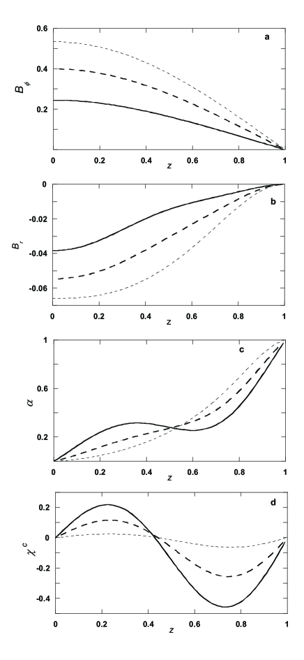
Figure 1: The $z$-dependence of solutions for the one-dimensional model; dynamo number $D=-20$, $C=1$, $\kappa=1$ and $|\chi^{v}(z)|=\sin^{2}(\pi z/2)$. The various curves indicate results with $h/l=2$ (short-dashed), $h/l=5$ (dashed) and $h/l=10$ (solid). a) the toroidal magnetic field $B_{\phi}(z)$, b) the poloidal magnetic field $B_{r}(z)$, c) the total $\alpha$-effect, $\alpha(z)$, d) the function $\chi^{c}(z)$.

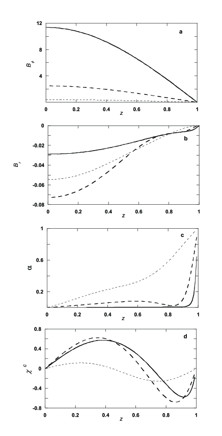
Figure 2: As Fig. 1, with $h/l=5$, and dynamo numbers $D=-20$ (short-dashed), $D=-100$ (dashed) and $D=-1000$ (solid).

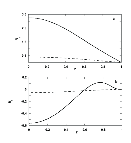
Figure 3: As Fig. 1, with $D=-20$, showing the effects of changing $C$: $C=1$ (dashed) and $C=10$ (solid); $h/l=5$.

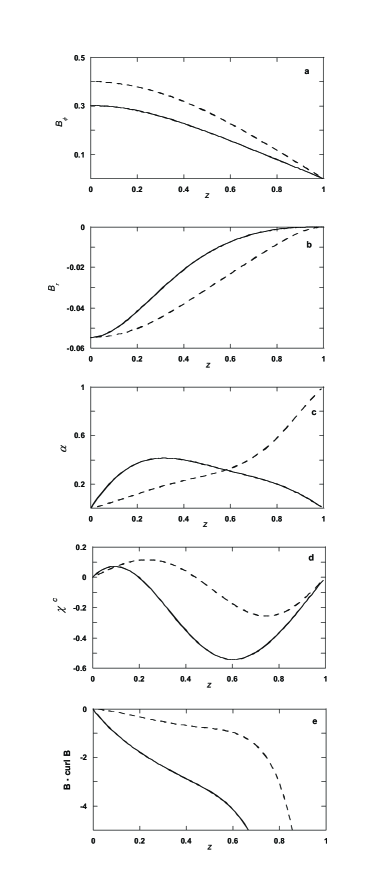
Figure 4: As Fig. 1, with $D=-20$, $C=1$, $h/l=5$, showing the effects of changing the form of $\chi^{v}$: $|\chi^{v}(z)|=\sin^{2}(\pi z/2)$ (dashed), and $\chi^{v}(z)=\sin(\pi z)$ (solid).

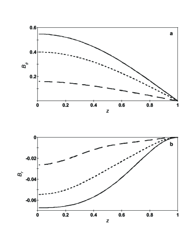
Figure 5: As Fig. 1, with $D=-20$, $C=1$, $h/l=5$, $|\chi^{v}(z)|=\sin^{2}(\pi z/2)$, showing the effects of changing $\kappa$: $\kappa=0.1$ (dashed), $\kappa=1$ (short-dashed), $\kappa=10$ (solid). The values of $\chi^{c}$ vary in the ranges $(-0.5,0.25)$, $(-0.25,0.10)$ and $(-0.04,0.15)$ for $\kappa=0.1,\,1$ and 10 respectively.

However, it is clear that a detailed agreement with observed galactic magnetic fields needs some effort. In many cases we obtain a steady-state magnetic field about $0.1-0.5B_{\rm eq}$ while observations suggest $B\approx B_{\rm eq}$. To get this we need $|D|>20-100$ (Fig. 2), which is a quite restrictive condition, or a value of $C$ that exceeds unity (Fig. 3). However straightforward theoretical estimations suggest $C<1$. Even so, the values of $C$ required do not appear unreasonable, given the inherent uncertainties of the theory.

5 The no-$z$ model

5.1 The model equations

The basic no-$z$ dynamo model for disc galaxies is described in Moss (1995). Phillips (2001) suggested a plausible tuning of the model and his major amendment, the multiplication by factors $\pi^{2}/4$ of the terms representing the $z$-diffusion of $B_{r}$ and $B_{\phi}$, was implemented here. The no-$z$ model differs from the local model of Sect. 3 in that it describes magnetic fields over the entire radial range, $0\leq r\leq R$, but all explicit dependence on the vertical coordinate $z$ has been removed, with $z$-derivatives being replaced by inverse powers of $h$. The field components $B_{r}$, $B_{\phi}$ appearing in the no-$z$ equations can either be thought of as representing mid-plane values, or as some sort of vertical average of values through the disc. Here we develop a version of Eq. (12) for the no-$z$ model, starting from the appropriate analogue of Eq. (12) which is

$${{\partial\chi^{c}}\over{\partial t}} = \rho(r)^{-1}\biggl{\{}4\biggl{(}{h\over l}\biggr{)}^{2}\biggl{[}R_{\alpha}^{-1}\@vec{B}\,\cdot(\@vec{\nabla}\times\@vec{B})-\alpha B^{2}$$ (25)

$$-{\rm div}\biggl{(}{\@vec{\nabla}\rho\over\rho}\,\chi^{v}\,B^{2}\Phi_{v}(B/\sqrt{\rho})\biggr{)}\biggr{]}$$

$$+\Delta\chi^{c}-{\rm div}[\@vec{V}\,\chi^{c}]\biggr{\}}\;,$$

$$\alpha = \chi^{v}\,\Phi_{v}(B/\sqrt{\rho})+\chi^{c}\,\Phi_{m}(B/\sqrt{\rho})\;,$$ (26)

where $\@vec{V}=\@vec{e}_{\phi}\,\Omega\,r$ is the large-scale velocity (differential rotation). The factor $\rho^{-1}$ multiplying by the right hand side of Eq. (25) arises because the link between the magnetic helicity $\chi^{m}$ and the current helicity $\chi^{c}$ contains the density $\rho,$ i.e. $\chi^{c}=\chi^{m}/18\pi\eta_{T}\rho.$ The quenching functions $\Phi_{v}$ and $\Phi_{m}$ contain in their arguments the factor $1/\sqrt{\rho}$ because they are based on local equipartition, while Eqs. (25) and (26) presume that the field $B$ is measured in units of equipartition at the point $r=0$. Note that our model includes a flux of magnetic helicity which is not directly connected with a mean magnetic energy flux; however an energy flux associated with the small-scale magnetic field is, of course, possible.

The coordinate version of Eq. (25) is given by

$${\partial\chi^{c}\over\partial t} = \rho^{-1}\biggl{\{}4\biggl{(}{h\over l}\biggr{)}^{2}[R_{\alpha}^{-1}(B_{\phi}B_{r}^{\prime}-B_{r}B^{\prime}_{\phi})-\alpha B^{2}$$ (27)

$$+(|\chi^{v}|\,\Phi_{v}\,B^{2})^{\prime}]+{4\lambda^{2}\over r}{\partial\over\partial r}[r\,\chi^{v}\,\Lambda_{\rho}^{-1}\,\Phi_{v}\,B^{2}]+(\chi^{c})^{\prime\prime}$$

$$+{\lambda^{2}\over r}{\partial\over\partial r}\biggl{(}r{\partial\chi^{c}\over\partial r}\biggr{)}+{\lambda^{2}\over r^{2}}{\partial^{2}\chi^{c}\over\partial\phi^{2}}-\lambda^{2}\Omega{\partial\chi^{c}\over\partial\phi}\biggr{\}}\;,$$

where $(\chi^{c})^{\prime}=\partial\chi^{c}/\partial z$, $\lambda=h/R$ is the aspect ratio, and $\Lambda^{-1}_{\rho}=-|\@vec{\nabla}|\rho/\rho$ is the density stratification scale.

For the no-z model in the axisymmetric case Eq. (27) becomes

$${\partial\chi^{c}\over\partial t} = \rho^{-1}\biggl{\{}4\biggl{(}{h\over l}\biggr{)}^{2}[R_{\alpha}^{-1}\zeta B_{r}B_{\phi}+C\,\chi^{v}\,\Phi_{v}(B/\sqrt{\rho})\,B^{2}$$ (28)

$$-\alpha B^{2}]-\kappa\chi^{c}+{4\lambda^{2}\over r}{\partial\over\partial r}[r\,\Lambda_{\rho}^{-1}\,\chi^{v}\,\Phi_{v}(B/\sqrt{\rho})\,B^{2}]$$

$$+{\lambda^{2}\over r}{\partial\over\partial r}\biggl{(}r\,{\partial\chi^{c}\over\partial r}\biggr{)}\biggr{\}}\;.$$

Note that with the no-$z$ formalism, the term $\@vec{B}\,\cdot(\@vec{\nabla}\times\@vec{B})$ vanishes identically. Examination of the solutions of Sect. 4.2 suggests that setting this term to zero may not always be a good approximation, but experimentation with the inclusion of an order of magnitude estimate for the omitted term suggests that the no-$z$ solutions are insensitive to it. We have introduced a coefficient $\kappa$ in the term $-\kappa\,\chi^{c}$ in Eq. (28). The motivation is that this term represents the term $\partial^{2}\chi^{c}/\partial z^{2}$ in Eq. (27). The literal application of the no-$z$ rules would imply $\kappa=1$. However the results of Sect. 4.2 suggest that in the local model $\chi^{c}\sim\sin(2\pi z)$, giving $\kappa\approx 4\pi^{2}$. This is analogous to the modification of the representation of the $z$-diffusion terms for the magnetic field suggested by Phillips (2001), and mentioned above. Thus we introduce $\kappa$ as a free parameter. The term $\chi^{v}\,\Phi_{v}(B/\sqrt{\rho})\,B^{2}$ represents a magnetic helicity flux. As it is introduced in a somewhat ad hoc manner, we have introduced the coefficient $C$ to represent this uncertainty. To determine the magnetic field distribution along the radius we use a Brandt rotation law, $\Omega(r)=\Omega_{0}/[1+(r/r_{\omega})^{2}]^{1/2}$ with $r_{\omega}=0.2,$ and the radial density profile $\rho(r)=\exp[-(r/r_{\rho})^{2}]$ with $r_{\rho}=0.5$, so that $\Lambda_{\rho}=2r/r_{\rho}^{2}.$ We also set $\chi^{v}(r)=1.$

One technical point should be noted here, which is important when comparing results from the local thin-disc model, studied in the earlier parts of this paper, with those from the no-$z$ model. For the local thin-disc model, $R_{\omega}=rh^{2}\eta_{T}^{-1}d\Omega/dr<0$. By the nature of the model, $rd\Omega/dr$ is the value at a chosen radius in the disc, and $r$ does not further occur explicitly in the analysis. However the no-$z$ model is global with respect to radius, and the value of $rd\Omega/dr$ varies through the disc, from zero at $r=0$ to some maximum absolute value; for the Brandt rotation law this value is $0.31\Omega_{0}$ at $r=\sqrt{2/3}r_{\omega}$. For the no-$z$ model the global definition is $R_{\omega}=R_{\omega}({\rm no}-z)=\Omega_{0}h^{2}/\eta_{T}>0$. (Less importantly, there are also small differences, of order 25%, in the effective values of $R_{\alpha}$ occurring in the two approximations, even though the formal definitions are the same - see Phillips (2001).) To emphasize these distinctions, we write the no-$z$ dynamo number as ${\cal D}=R_{\omega}({\rm no}-z)R_{\alpha}$.

For these reasons, it cannot be expected that there will be a precise correspondence between the values of the marginal dynamo numbers for these two approximations; empirically we found ${\cal D}_{\rm crit}\approx 20$. We note that $|D_{\rm crit}|/{\cal D}_{\rm crit}\approx 0.4$, which can be compared with the maximum value of $|rd\Omega/dr|/\Omega_{0}=0.31$ for the no-$z$ model with our Brandt rotation law. These issues are also touched on in Sects. 3.2 and 4 of Moss et al. (2001).

What seem to be important are the terms with $\lambda^{2}.$ They represent a diffusion and an advection of helicity along the radius, i.e. from the galactic center to its periphery. This could lead to a more extended magnetic field distribution than given by conventional models. This is why the result can be compared with that from the conventional model with $\alpha\sim 1/(1+B^{2}/\rho).$

5.2 Numerical results

We integrated the standard axisymmetric no-$z$ equations (modified as described above) for $B_{r}$ and $B_{\phi}$, together with Eq. (28), from arbitrarily chosen initial conditions for a range of values of $C$ and $\kappa$, finding steady solutions. We present in Fig. 6, as examples which are close enough to the available phenomenology of galactic magnetic fields, solutions with $\kappa=1$, $\zeta=0$, ${\cal D}=50$, $C=3$ (dashed line) and $C=10$ (solid line).

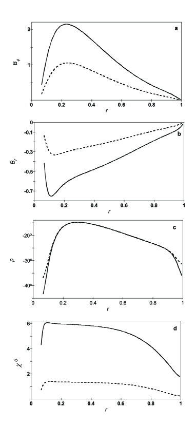
Figure 6: Details of the no-$z$ model, with dynamo number ${\cal D}=50$, $h/l=5$, $\lambda=0.05$, $|\chi^{v}(z)|=\sin^{2}(\pi z/2)$. a) the toroidal magnetic field $B_{\phi}(r)$, b) the radial magnetic field $B_{r}(r)$, c) the pitch angle $p$, d) the function $\chi^{c}(z)$. Broken curves are solutions with $C=3$, solid with $C=10$.

Again, we can observe that typically $|\@vec{B}|$ is of order unity. The value $r=1$ can be taken roughly to correspond to 15 kpc in dimensional units, so the radial magnetic field reaches its maximal value at a galactocentric radius of $3\dots 4$ kpc, quite typical for the simplest approximations of galactic rotation curves. Pitch angles in this radial range are about $-15^{\circ}\dots-20^{\circ}$, in agreement with available observational data. The values of $\chi^{c}$ are in the range $1.5\dots 6$, so the back reaction of magnetic field basically modifies the dynamo action. The main dependencies of the results on the model parameters are given in Table 1.

We conclude from the the results shown in Table 1 that in the no-$z$ model the helicity diffusivity $\kappa$ does not play an important role (in contrast to the 1D model of the previous section). The only anomalous thing about solutions with $\kappa=0$ is an extremely long (about 50 diffusion times) transient phase when $C=0.1$. However this was not a slow growth, but rather a growth over a few time units followed by a rapid decay and then a slow relaxation. This feature was not seen when $C=1,10$, when the magnetic fields grew to approximately their final strengths over a few time units.

Table 1: Summary of selected calculations for the no-$z$ model. $E_{r}/E_{\phi}$ is the ratio of energies in the radial and azimuthal magnetic fields, $\langle p\rangle$ and $\langle\chi^{c}\rangle$ are the averages with respect to radius of pitch angle (in degrees) and $\chi^{c}$ in the range $0.20<r<0.80$, and $B_{\phi,m}$ is the maximum value of $B_{\phi}$.

Table 1.
$R_{\alpha}=2$, $R_{\omega}=25$, ${\cal D}=50$
$C=0.1$
$\kappa$	$E_{r}/\bar{E}_{\phi}$	$\langle p\rangle$	$\langle\chi^{c}\rangle$	$B_{\phi,m}$
0	0.089	$-16$	$-0.67$	0.028
0.1	0.118	$-18$	$-0.56$	0.060
1.0	0.113	$-18$	$-0.42$	0.149
10.0	0.103	$-18$	$-0.18$	0.320
$C=1.0$
0, 0.1, 1.0, 10.0	0.097	$-18$	$\approx 0$	0.484
$C=10.0$
0	0.104	$-18$	6.22	2.19
0.1	0.103	$-18$	6.1	2.19
1.0	0.100	$-18$	5.5	2.15
10.0	0.096	$-18$	2.9	0.82
$C=-1.0$
1.0	0.13	$-18$	-0.52	0.073
10.0	0.11	$-18$	-0.30	0.021
$R_{\alpha}=5$, $R_{\omega}=80$, ${\cal D}=400$
$C=1.0$
0.1, 1.0, 10.0	0.01	$-6$	$\approx 0$	1.93

The interaction of the two flux transport coefficients is not straightforward. For $C=0.1$, field strengths increase with $\kappa$, whereas for $C=10$, they decrease. When $C=1.0$, the solutions are remarkably insensitive to the value of $\kappa$, independent of the value of ${\cal D}$. These comments apply both to solutions with a modestly supercritical dynamo number (${\cal D}=50$), and a very supercritical ${\cal D}=400$. The pitch angle depends predominantly on ${\cal D}$ – see Table 1.

6 Discussion and conclusions

Conventional galactic dynamo models are based usually on a naive concept of $\alpha$-quenching. From the theoretical point of view this concept must sooner or later be replaced by a better elaborated model for the processes of magnetic helicity generation and transport, which lead to dynamo saturation. In this paper we have presented a model of such saturation, based as far as possible physically on first principles rather than on ad hoc parameterizations of turbulence. This model is shown to reproduce successfully basic features of galactic magnetic fields and, when used in conjunction with standard galactic dynamo models, can be used to obtain detailed models of magnetic field generation in specific galaxies. Perhaps not unexpectedly, we have to adjust some coefficients of the model in order to obtain this agreement. However all terms occurring in the model can be justified from first principles.

Magnetic field distributions obtained with our model are compared with that from a model with a conventional $\alpha$-quenching and corresponding values of the control parameters, in Fig. 7. It can be seen that results for these models closely resemble each other, and for the choice $C=3$ they practically coincide; certainly their deviation is much less than the available accuracy of the observations. Note that our model, in the case shown in Fig. 7, is intrinsically quite distant from an $\alpha$-quenched model. However, for $C=1.0$ and ${\cal D}=-50$ we find $\langle\chi^{c}\rangle\approx 0$, so here the dynamo saturation must be connected mainly with a conventional $\alpha$-quenching and $\kappa$ has no influence. We take here $\kappa=1$ although, as noted, solutions are insensitive to $\kappa$ for these parameters. Of course, the last result does not coincide with that for conventional $\alpha$-quenching, because Eq. (28) is more complicated than the conventional $\alpha$-quenching, even when $\langle\chi^{c}\rangle\approx 0$.

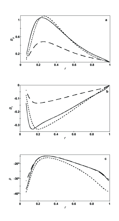
Figure 7: Comparison of the equilibrium $r$-profiles for the no-$z$ model obtained using two kinds of nonlinearities: the nonlinearity considered here for $C=1$ (dashed) and $C=3$ (solid), and a standard alpha-quenching $\alpha\propto 1/[1+B^{2}(\@vec{r})/\rho(r)]$ with $\rho=1$ (short-dashed). Notation is as in Fig. 6.

From a practical viewpoint, these results lead to a two-fold conclusion. On one hand the research undertaken can be considered as a justification of conventional galactic dynamo models based on a naive $\alpha$-quenching. However the physics underlying our model is much more complicated. On the other hand it means that the galactic dynamo, at least in its standard manifestation considered here, is very robust and the resulting magnetic field is practically independent of small details of the dynamo model. It follows that it is necessary to consider more fragile dynamo regimes in order to isolate features specifically connected with the details of dynamo saturation mechanisms.

Our analysis has also shown that the detailed form of the flux of the magnetic helicity is not crucial for the overall state of the saturated mean magnetic field. The most important factor is to have a nonzero flux of the magnetic helicity (e.g., in the form of the transport term or in the form of the diffusive term).

We note that our results clarify the role of magnetic helicity transport in galactic dynamos in the mean-field approach only. However, we do not address the question of the link between the transport of the total magnetic helicity $\@vec{\cal A}\cdot\@vec{H}$ and the total magnetic field $\@vec{H}$. A recent paper by Brandenburg et al. (2001b) on the topic of stellar dynamos using direct numerical simulations isolates many further questions which are still far from being clear.

Finally, we note that theoretical ideas do not even exclude negative values of $C$. In this case larger steady state magnetic fields might be predicted, because the flux transport could then amplify the mean field and the saturation might be connected with the diffusive flux only. However the results of simulations with negative $C$ given in Table 1 demonstrate that the detailed balance between the various terms in Eq. (28) is too complicated for this simple explanation to be valid.

- (1) Beck, R., Brandenburg, A., Moss, D., Shukurov, A., & Sokoloff, D. 1996, ARA&A, 34, 155
- (2) Blackman, E., & Field, G. 2000, ApJ, 534, 984
- (3) Brandenburg A., 2001, ApJ 550,824
- (4) Brandenburg, A., Bigazzi, A., & Subramanian, K. 2001a, MNRAS, 325, 685
- (5) Brandenburg, A., Dobler, W., & Subramanian, K., 2001b, astro-ph/0111576
- (6) Chae, J. 2001, ApJ, 560, L95
- (7) Covas, E., Tavakol, R., Tworkowski, A., & Brandenburg, A. 1998, A&A, 329, 350
- (8) Field, G., Blackman, E., & Chou, H. 1999, ApJ, 513, 638
- (9) Frisch U., Pouquet A., Leorat I., & Mazure A., 1975, J. Fluid Mech. 68, 769
- (10) Gruzinov, A. V., & Diamond, P. H. 1995, Phys. Plasmas, 2, 1941
- (11) Iroshnikov, R. S. 1970, SvA, 14, 582; 1001
- (12) Kleeorin, N., Moss, D., Rogachevskii, I., & Sokoloff, D. 2000, A&A, 361, L5
- (13) Kleeorin, N., & Rogachevskii, I. 1999, Phys. Rev. E., 59, 6724
- (14) Kleeorin, N., Rogachevskii, I., & Ruzmaikin, A. 1995, A&A, 297, 159
- (15) Kleeorin, N., & Ruzmaikin, A., 1982, Magnetohydrodyn., 18, 116
- (16) Kulsrud, R. 1999, Ann. Rev. Astron. Astrophys., 37, 37
- (17) Moss, D. 1995, MNRAS, 275, 191
- (18) Moss, D., Shukurov, A., & Sokoloff, D. 1999, A&A, 343, 120.
- (19) Moss, D., Shukurov, A., Sokoloff, D., Beck, R., & Fletcher, A. 2001, A&A, 3380, 55.
- (20) Parker, E. N. 1992, ApJ, 163, 252.
- (21) Phillips, A. 2001, GAFD, 94, 135
- (22) Roberts, P. N., & Soward, A. M. 1975, Astron. Nachr., 296, 49
- (23) Rogachevskii, I., & Kleeorin, N. 2000, Phys. Rev. E., 61, 5202
- (24) Rogachevskii, I., & Kleeorin, N. 2001, Phys. Rev. E., 64, 056307
- (25) Rüdiger, G. 1974, Astron. Nachr., 295, 229
- (26) Ruzmaikin, A., Shukurov, A., & Sokoloff, D. 1988, Magnetic Fields of Galaxies (Kluwer, Dordrecht)
- (27) Schmalz, S., & Stix, M. 1991, A&A, 245, 654
- (28) Vainshtein, S. I., & Cattaneo, F. 1992, ApJ, 393, 165
- (29) Vishniac, E. T., & Cho, J. 2001, ApJ, 550, 752
- (30) Zeldovich, Ya. B., Ruzmaikin, A. A., & Sokoloff, D. D. 1983, Magnetic Fields in Astrophysics (Gordon and Breach, New York)