New Understanding of Large Magellanic Cloud Structure, Dynamics and Orbit from Carbon Star Kinematics

Abstract

We formulate a new, revised and coherent understanding of the structure and dynamics of the Large Magellanic Cloud (LMC), and its orbit around and interaction with the Milky Way. Much of our understanding of these issues hinges on studies of the LMC line-of-sight kinematics. The observed velocity field includes contributions from the LMC rotation curve $V(R^{\prime})$, the LMC transverse velocity vector ${\vec{v}}_{t}$, and the rate of inclination change $di/dt$. All previous studies have assumed $di/dt=0$. We show that this is incorrect, and that combined with uncertainties in ${\vec{v}}_{t}$ this has led to incorrect estimates of many important structural parameters of the LMC. We derive general expressions for the velocity field which we fit to kinematical data for 1041 carbon stars. We calculate ${\vec{v}}_{t}$ by compiling and improving LMC proper motion measurements from the literature, and we show that for known ${\vec{v}}_{t}$ all other model parameters are uniquely determined by the data. The position angle of the line of nodes is $\Theta=129.9^{\circ}\pm 6.0^{\circ}$, consistent with the value determined geometrically by van der Marel & Cioni (2001). The rate of inclination change is $di/dt=-0.37\pm 0.22\>{\rm mas}\,{\rm yr}^{-1}=-103\pm 61$ degrees/Gyr. This is similar in magnitude to predictions from $N$-body simulations by Weinberg (2000), which predict LMC disk precession and nutation due to Milky Way tidal torques. The LMC rotation curve $V(R^{\prime})$ has amplitude $49.8\pm 15.9\>{\rm km}\,{\rm s}^{-1}$. This is $40$% lower than what has previously (and incorrectly) been inferred from studies of HI, carbon stars, and other tracers. The line-of-sight velocity dispersion has an average value $\sigma=20.2\pm 0.5\>{\rm km}\,{\rm s}^{-1}$, with little variation as function of radius. The dynamical center of the carbon stars is consistent with the center of the bar and the center of the outer isophotes, but it is offset by $1.2^{\circ}\pm 0.6^{\circ}$ from the kinematical center of the HI. The enclosed mass inside the last data point is $M_{\rm LMC}(8.9\>{\rm kpc})=(8.7\pm 4.3)\times 10^{9}\>{\rm M_{\odot}}$, more than half of which is due to a dark halo. The LMC has a considerable vertical thickness; its $V/\sigma=2.9\pm 0.9$ is less than the value for the Milky Way’s thick disk ($V/\sigma\approx 3.9$). Simple arguments for models stratified on spheroids indicate that the (out-of-plane) axial ratio could be $\sim 0.3$ or larger. Isothermal disk models for the observed velocity dispersion profile confirm the finding of Alves & Nelson (2000) that the scale height must increase with radius. A substantial thickness for the LMC disk is consistent with the simulations of Weinberg, which predict LMC disk thickening due to Milky Way tidal forces. These affect LMC structure even inside the LMC tidal radius, which we calculate to be $r_{t}=15.0\pm 4.5\>{\rm kpc}$ (i.e., $17.1^{\circ}\pm 5.1^{\circ}$). The new insights into LMC structure need not significantly alter existing predictions for the LMC self-lensing optical depth, which to lowest order depends only on $\sigma$. The compiled proper motion data imply an LMC transverse velocity $v_{t}=406\>{\rm km}\,{\rm s}^{-1}$ in the direction of position angle $78.7^{\circ}$ (with errors of $\sim 40\>{\rm km}\,{\rm s}^{-1}$ in each coordinate). This can be combined with the observed systemic velocity, $v_{\rm sys}=262.2\pm 3.4\>{\rm km}\,{\rm s}^{-1}$, to calculate the LMC velocity in the Galactocentric rest frame. This yields $v_{\rm LMC}=293\pm 39\>{\rm km}\,{\rm s}^{-1}$, with radial and tangential components $v_{\rm LMC,rad}=84\pm 7\>{\rm km}\,{\rm s}^{-1}$ and $v_{\rm LMC,tan}=281\pm 41\>{\rm km}\,{\rm s}^{-1}$, respectively. This is consistent with the range of velocities that has been predicted by models for the Magellanic Stream. The implied orbit of the LMC has an apocenter to pericenter distance ratio $\sim 2.5:1$, a perigalactic distance $\sim 45\>{\rm kpc}$, and a present orbital period around the Milky Way $\sim 1.5\>{\rm Gyr}$. The constraint that the LMC is bound to the Milky Way provides a robust limit on the minimum mass and extent of the Milky Way dark halo: $M_{\rm MW}\geq 4.3\times 10^{11}\>{\rm M_{\odot}}$ and $r_{h}\geq 39\>{\rm kpc}$ (68.3% confidence). Finally, we present predictions for the LMC proper motion velocity field, and we discuss how measurements of this may lead to kinematical distance estimates of the LMC.

1 Introduction

The Large and Small Magellanic Clouds (LMC and SMC) are close companion galaxies of our Milky Way. Their interaction with the Milky Way has produced the Magellanic Stream, which spans more than $100^{\circ}$ across the sky (e.g., Westerlund 1997; Wakker 2002). It consists of gas that trails the Magellanic Clouds as they orbit the Milky Way. A less prominent leading gas component was recently discovered as well (Lu et al. 1998; Putman 1998). Models of the Magellanic Stream hold the promise of providing important constraints on the mass and gravitational potential of the Milky Way dark halo (e.g., Lin, Jones & Klemola 1995). However, this requires an accurate understanding of the three-dimensional velocity of the Magellanic Clouds. While the systemic line-of-sight velocities of both the LMC and SMC have been accurately determined using Doppler shifts, a determination of their transverse velocities in the plane of the sky has proven to be much more difficult. We restrict our attention in the present paper to the LMC, which has been studied more and is understood better than the SMC. Several proper motion studies of the LMC have been published (Jones, Klemola & Lin 1994; Kroupa, Röser & Bastian 1994; Kroupa & Bastian 1997; Drake et al. 2002; Pedreros, Anguita & Maza 2002), but the uncertainties in the measurements are considerable. Accurate knowledge of the LMC transverse velocity has therefore remained elusive.

The uncertainty in the transverse velocity of the LMC has not only restricted models of the Magellanic Stream, but also the interpretation of the observed LMC line-of-sight velocity field. As one moves away from the LMC center, the transverse velocity component of the LMC center of mass (CM) ceases to be perpendicular to the line of sight. This causes a spurious solid-body rotation component in the observed line-of-sight velocity field (Feast, Thackeray & Wesselink 1961). Initially this effect was used to obtain a rough estimate of the transverse velocity of the LMC under the assumption (appropriate for a circular disk) that its kinematic line of nodes (defined as the line of maximum velocity gradient) should be equal to the photometric major axis (Feitzinger, Schmidt-Kaler & Isserstedt 1977; Meatheringham et al. 1988; Gould 2000). However, this assumption is now known to be invalid. Robust geometric methods show that the line of nodes of the LMC (defined as the intersection of the galaxy-plane and the sky-plane) does not coincide with the photometric major axis (van der Marel & Cioni 2001, hereafter Paper I), and hence, that the LMC is intrinsically elongated (van der Marel 2001, hereafter Paper II). The most recent analyses of the LMC velocity field have corrected for the spurious solid-body rotation component using the available LMC proper motion measurements (e.g., Kim et al. 1998; Alves & Nelson 2000). However, the corrections involved are large (because the spurious component is comparable to the intrinsic LMC rotation component) and highly uncertain (because the LMC proper motion is not known accurately). In addition, all previous studies have assumed that the LMC viewing angles have no explicit time dependence, contrary to the results of $N$-body simulations which predict precession and nutation of the LMC disk due to Milky Way tidal torques (Weinberg 2000). All this probably explains why analyses of the LMC velocity field have yielded somewhat puzzling results. For example, Alves & Nelson (2000) obtained from a study of carbon-star velocities that the position angle of the kinematic line of nodes rises from $\Theta_{\rm kin}=143^{\circ}\pm 7^{\circ}$ at a mean distance of $4.5^{\circ}$ from the galaxy center to $\Theta_{\rm max}=183^{\circ}\pm 8^{\circ}$ at $9.2^{\circ}$. The results obtained from HI kinematics by Kim et al. (1998) were qualitatively not very different. A kinematic twist of $40^{\circ}\pm 11^{\circ}$ is quite unexpected, given that, over the same range of distances, the LMC has no twist in the stellar number density contours (to an accuracy of $\sim 3^{\circ}$; Paper II). More importantly, the inferred kinematic line of nodes differs considerably from the true line of nodes, for which a position angle $\Theta=122.5\pm 8.3^{\circ}$ was determined geometrically from DENIS and 2MASS near-IR stellar catalogs (Paper I). While the LMC is not intrinsically circular, the implied difference between $\Theta$ and $\Theta_{\rm kin}$ is too large to plausibly attribute to non-circular orbits (Paper II).

In the present paper we address these issues, and their consequences, by presenting the most detailed and sophisticated analysis to date of the LMC line-of-sight velocity field. In Section 2 we derive general expressions for the velocity fields of a rotating disk galaxy that has a non-negligible angular extent on the sky, both for the line-of-sight velocity component and for the velocity components in the plane of the sky. In Section 3 we present a conceptual discussion of the line-of-sight velocity field. We address which quantities are uniquely constrained by the observations, and which ones are not. In Section 4 we fit the general equations for the line-of-sight velocity field to the velocities available for 1041 carbon stars, and we discuss the results. In Section 5 we review what is known about the proper motion and distance of the LMC from other sources. In Section 6 we combine this knowledge with the information obtained from the analysis of the line-of-sight velocity field to determine $di/dt$, the rate at which the LMC inclination changes with time. In Section 7 we discuss the kinematical properties of the LMC disk as implied by our analysis. We address the position of the dynamical center, the disk rotation curve and the velocity dispersion profile, the position angle of the line of nodes, and the influence of non-circular orbits on the results of the analysis. In Section 8 we discuss the implications of the results for our understanding of the structure of the LMC, including its mass, tidal radius, scale height, dark halo and self-lensing optical depth. In Section 9 we discuss the implications of the results for the transverse velocity of the LMC, the three-dimensional velocity of the LMC in the Galactocentric rest frame, the orbit of the LMC around the Milky Way, the mass and extent of the Milky Way, and the origin of the Magellanic Stream. In Section 10 we present predictions for the proper motion velocity field of the LMC, which may be observationally accessible with future astrometric missions. In Section 11 we discuss a new method for kinematical determination of the LMC distance, and its prospects for yielding results that are competitive with other methods. Conclusions are presented in Section 12. Appendix A discusses an improved analysis of the published proper measurements of Jones et al. (1994) and Pedreros et al. (2002), which were obtained for fields that are offset from the LMC CM.

2 General Expressions for the Velocity Field of a Rotating Disk

Many previous studies have given equations for the description of the velocity field of an external galaxy. However, it is customary to make the assumption that the angular size subtended by the galaxy is negligible. This is equivalent to assuming that the galaxy is at infinite distance and that ‘the sky is flat’ over the area of the galaxy. However, the LMC subtends a very large angle on the sky (more than $20^{\circ}$ end-to-end) and this makes the usual equations inadequate for describing its kinematics. We therefore start by deriving general expressions for the velocity field of a rotating disk which are valid for a galaxy of arbitrary angular size. We address not only the line-of-sight velocities, but also the velocity components perpendicular to the line of sight. Readers interested mostly in the application to the LMC may wish to skip directly to Section 3.

2.1 Coordinate Systems and Velocity Components

We adopt the same coordinate systems as in Paper I. The position of any point in space is uniquely determined by its right ascension and declination on the sky, $(\alpha,\delta)$, and its distance $D$. The point ${\cal O}$ with coordinates $(\alpha_{0},\delta_{0},D_{0})$ is the origin of the analysis, and is chosen to be the galaxy center of mass (CM). Angular coordinates $(\rho,\phi)$ are defined on the celestial sphere, where $\rho$ is the angular distance between the points $(\alpha,\delta)$ and $(\alpha_{0},\delta_{0})$, and $\phi$ is the position angle of the point $(\alpha,\delta)$ with respect to $(\alpha_{0},\delta_{0})$; see Figure 1. In particular, $\phi$ is the angle at $(\alpha_{0},\delta_{0})$ between the tangent to the great circle on the celestial sphere through $(\alpha,\delta)$ and $(\alpha_{0},\delta_{0})$, and the circle of constant declination $\delta_{0}$. By convention, $\phi$ is measured counterclockwise starting from the axis that runs in the direction of decreasing right ascension at constant declination $\delta_{0}$. Equations (1)–(3) of Paper I allow $(\rho,\phi)$ to be calculated for any $(\alpha,\delta)$.

At any given position $(D,\rho,\phi)$, a velocity vector can be decomposed into a sum of three orthogonal components:

$$v_{1}\equiv{{dD}\over{dt}},\qquad v_{2}\equiv D{{d\rho}\over{dt}},\qquad v_{3}\equiv D\sin\rho{{d\phi}\over{dt}}.$$ (1)

Here, $v_{1}$ is the line-of-sight velocity, and $v_{2}$ and $v_{3}$ are the velocity components in the plane of the sky; see Figure 2. The goal of the present analysis is to obtain expressions for $(v_{1},v_{2},v_{3})$ as a function of $(\rho,\phi)$.

We introduce a Cartesian coordinate system $(x,y,z)$ that has its origin at ${\cal O}$, with the $x$-axis anti-parallel to the RA axis, the $y$-axis parallel to the declination axis, and the $z$-axis towards the observer; see Figures 1 and 2. The transformation equations from $(D,\rho,\phi)$ to $(x,y,z)$ are given by equation (5) of Paper I. The inverse transformation equations are:

$$D = [x^{2}+y^{2}+(D_{0}-z)^{2}]^{1/2},$$

$$\rho = \arctan[(x^{2}+y^{2})/(D_{0}-z)^{2}]^{1/2},$$ (2)

$$\phi = \arctan(y/x).$$

Substitution of equation (2.1) in equation (1) yields after some manipulations

$$\left(\begin{array}[]{c}v_{1}\\ v_{2}\\ v_{3}\end{array}\right)=\left(\begin{array}[]{ccc}\sin\rho\cos\phi&\sin\rho\sin\phi&-\cos\rho\\ \cos\rho\cos\phi&\cos\rho\sin\phi&\sin\rho\\ -\sin\phi&\cos\phi&0\end{array}\right)\>\left(\begin{array}[]{c}v_{x}\\ v_{y}\\ v_{z}\end{array}\right),$$ (3)

where $(v_{x},v_{y},v_{z})$ is the three-dimensional velocity in the $(x,y,z)$ coordinate system. To describe the internal kinematics of the galaxy it is useful to adopt a second Cartesian coordinate system $(x^{\prime},y^{\prime},z^{\prime})$ that is obtained from the system $(x,y,z)$ by counterclockwise rotation around the $z$-axis by an angle $\theta$, followed by a clockwise rotation around the new $x^{\prime}$-axis by an angle $i$; see Figure 3. With this definition, the $(x^{\prime},y^{\prime})$ plane is inclined with respect to the sky by the angle $i$ (with face-on viewing corresponding to $i=0$). The angle $\theta$ is the position angle of the line of nodes (the intersection of the $(x^{\prime},y^{\prime})$-plane and the $(x,y)$-plane of the sky), measured counterclockwise from the $x$-axis. In practice, $i$ and $\theta$ will be chosen such that the $(x^{\prime},y^{\prime})$ plane coincides with the equatorial plane of the galaxy. The transformation equations from $(x,y,z)$ to $(x^{\prime},y^{\prime},z^{\prime})$ are given by equation (6) of Paper I. The inverse transformations are

$$\left(\begin{array}[]{c}x\\ y\\ z\end{array}\right)=\left(\begin{array}[]{ccc}\cos\theta&-\sin\theta\cos i&-\sin\theta\sin i\\ \sin\theta&\cos\theta\cos i&\cos\theta\sin i\\ 0&-\sin i&\cos i\\ \end{array}\right)\>\left(\begin{array}[]{c}x^{\prime}\\ y^{\prime}\\ z^{\prime}\end{array}\right).$$ (4)

Upon taking the time derivative on both sides this yields transformation equations from $(v_{x}^{\prime},v_{y}^{\prime},v_{z}^{\prime})$ to $(v_{x},v_{y},v_{z})$. These can be substituted in equation (3), which after some further manipulations yields

$$\left(\begin{array}[]{c}v_{1}\\ v_{2}\\ v_{3}\end{array}\right)=\left(\begin{array}[]{ccc}\sin\rho\cos(\phi-\theta)&[\sin\rho\cos i\sin(\phi-\theta)+\cos\rho\sin i]&[\sin\rho\sin i\sin(\phi-\theta)-\cos\rho\cos i]\\ \cos\rho\cos(\phi-\theta)&[\cos\rho\cos i\sin(\phi-\theta)-\sin\rho\sin i]&[\cos\rho\sin i\sin(\phi-\theta)+\sin\rho\cos i]\\ -\sin(\phi-\theta)&\cos i\cos(\phi-\theta)&\sin i\cos(\phi-\theta)\\ \end{array}\right)\>\left(\begin{array}[]{c}v_{x}^{\prime}\\ v_{y}^{\prime}\\ v_{z}^{\prime}\end{array}\right).$$ (5)

For the analysis of the line-of-sight velocity field one needs only $v_{1}$, but to interpret proper motion measurements one needs to know in addition how the velocities $v_{2}$ and $v_{3}$ relate to the local directions of West and North. The proper motions in these directions are defined as

$$\mu_{W}=-\cos\delta({{d\alpha}/{dt}}),\qquad\mu_{N}=({{d\delta}/{dt}}).$$ (6)

To obtain expressions for these proper motions we start with equations (1)–(3) of Paper I, which relate $(\rho,\phi)$ to the right ascension and declination $(\alpha,\delta)$ on the sky. Upon taking the time derivative of these equations one obtains relations between ${{d\rho}/{dt}}$ and ${{d\phi}/{dt}}$ on the one hand, and ${{d\alpha}/{dt}}$ and ${{d\delta}/{dt}}$ on the other hand. These can be solved to obtain:

$$\left(\begin{array}[]{c}\mu_{W}\\ \mu_{N}\end{array}\right)=(1/D)\times\left(\begin{array}[]{cc}-\sin\Gamma&-\cos\Gamma\\ \cos\Gamma&-\sin\Gamma\\ \end{array}\right)\>\left(\begin{array}[]{c}v_{2}\\ v_{3}\end{array}\right).$$ (7)

The angle $\Gamma$ determines the rotation angle of the $(v_{2},v_{3})$ frame on the sky; see Figure 1. It is determined by

$$\cos\Gamma = [\sin\delta\cos\delta_{0}\cos(\alpha-\alpha_{0})-\cos\delta\sin\delta_{0}]\>/\sin\rho,$$

$$\sin\Gamma = [\cos\delta_{0}\sin(\alpha-\alpha_{0})]\>/\sin\rho.$$ (8)

In practice we restrict the discussion to a planar system with all tracers in the $(x^{\prime},y^{\prime})$ plane. In this case the distance $D$ to a tracer is related to the CM distance $D_{0}$ through equation (8) of Paper I. Substitution of that equation yields

$$\left(\begin{array}[]{c}\mu_{W}\\ \mu_{N}\end{array}\right)={{[\cos i\cos\rho-\sin i\sin\rho\sin(\phi-\theta)]}\over{D_{0}\cos i}}\times\left(\begin{array}[]{cc}-\sin\Gamma&-\cos\Gamma\\ \cos\Gamma&-\sin\Gamma\\ \end{array}\right)\>\left(\begin{array}[]{c}v_{2}\\ v_{3}\end{array}\right).$$ (9)

In practice one needs to express this in observable units, which is achieved by using the relation

$$v_{i}/D_{0}=\left\{(v_{i}/[\>{\rm km}\,{\rm s}^{-1}])\>/\>(4.7403885\>D_{0}/\>{\rm kpc})\right\}{\rm mas/yr}.$$ (10)

2.2 Velocity Field Model

For a planar system, the velocity of a tracer can be written as a sum of three components:

$$\left(\begin{array}[]{c}v_{1}\\ v_{2}\\ v_{3}\end{array}\right)=\left(\begin{array}[]{c}v_{1}\\ v_{2}\\ v_{3}\end{array}\right)_{{\rm CM}}+\left(\begin{array}[]{c}v_{1}\\ v_{2}\\ v_{3}\end{array}\right)_{{\rm pn}}+\left(\begin{array}[]{c}v_{1}\\ v_{2}\\ v_{3}\end{array}\right)_{{\rm int}}.$$ (11)

The first component, ${\vec{v}}_{{\rm CM}}$, is the velocity contributed by the space motion of the CM. The second component, ${\vec{v}}_{{\rm pn}}$, is the velocity contributed by time-variations in the viewing angles $i$ and $\theta$ of the disk plane. Such variations arise if the orientation of the disk plane is not static in an inertial frame. For the case of the LMC, this occurs naturally as a result of the precession and nutation of the disk plane induced by external tidal torques (Weinberg 2000). The third component, ${\vec{v}}_{{\rm int}}$, is the velocity contributed by the internal motion of the tracer in the disk plane. We proceed by deriving expressions for each of these contributions.

2.2.1 Center-of-Mass Motion

The velocity of the center of mass can be described by quantities $v_{\rm sys}$, $v_{t}$ and $\theta_{t}$, such that $v_{\rm sys}$ is the systemic velocity of the CM along the line of sight (positive when receding), $v_{t}$ is the transverse velocity of the CM, and $\theta_{t}$ is the direction of the transverse motion on the sky; see Figure 4. This implies

$$\left(\begin{array}[]{c}v_{x}\\ v_{y}\\ v_{z}\end{array}\right)_{{\rm CM}}=\left(\begin{array}[]{c}v_{t}\cos\theta_{t}\\ v_{t}\sin\theta_{t}\\ -v_{\rm sys}\end{array}\right).$$ (12)

From equations (3) and (12) one obtains for the observable velocity components

$$\left(\begin{array}[]{c}v_{1}\\ v_{2}\\ v_{3}\end{array}\right)_{{\rm CM}}=\left(\begin{array}[]{c}v_{t}\sin\rho\cos(\phi-\theta_{t})+v_{\rm sys}\cos\rho\\ v_{t}\cos\rho\cos(\phi-\theta_{t})-v_{\rm sys}\sin\rho\\ -v_{t}\sin(\phi-\theta_{t})\end{array}\right).$$ (13)

2.2.2 Precession and Nutation

To assess the effect of changes in $i$ and $\theta$, consider a point that has fixed coordinates in the $(x^{\prime},y^{\prime},z^{\prime})$ frame. By taking the time derivative of equation (4) one obtains:

$$\left(\begin{array}[]{c}v_{x}\\ v_{y}\\ v_{z}\end{array}\right)= (d\theta/dt) \left(\begin{array}[]{ccc}-\sin\theta&-\cos\theta\cos i&-\cos\theta\sin i\\ \cos\theta&-\sin\theta\cos i&-\sin\theta\sin i\\ 0&0&-\sin\theta\\ \end{array}\right)\>\left(\begin{array}[]{c}x^{\prime}\\ y^{\prime}\\ z^{\prime}\end{array}\right)+$$ (23)

$$(di/dt) \left(\begin{array}[]{ccc}0&\sin\theta\sin i&-\sin\theta\cos i\\ 0&-\cos\theta\sin i&\cos\theta\cos i\\ 0&-\cos i&0\\ \end{array}\right)\>\left(\begin{array}[]{c}x^{\prime}\\ y^{\prime}\\ z^{\prime}\end{array}\right).$$ (30)

For a planar disk ($z^{\prime}=0$), one has from equation (2) of Paper II:

$$\left(\begin{array}[]{c}x^{\prime}\\ y^{\prime}\\ z^{\prime}\end{array}\right)={{D_{0}\sin\rho}\over{\cos i\cos\rho-\sin i\sin\rho\sin(\phi-\theta)}}\left(\begin{array}[]{c}\cos i\cos(\phi-\theta)\\ \sin(\phi-\theta)\\ 0\end{array}\right).$$ (31)

These equations can be substituted in equation (3), which yields after some manipulations

$$\left(\begin{array}[]{c}v_{1}\\ v_{2}\\ v_{3}\end{array}\right)_{{\rm pn}}={{D_{0}\sin\rho}\over{\cos i\cos\rho-\sin i\sin\rho\sin(\phi-\theta)}}\left(\begin{array}[]{c}(di/dt)\sin(\phi-\theta)[\cos i\cos\rho-\sin i\sin\rho\sin(\phi-\theta)]\\ (di/dt)\sin(\phi-\theta)[-\cos i\sin\rho-\sin i\cos\rho\sin(\phi-\theta)]\\ (di/dt)\sin(\phi-\theta)[-\sin i\cos(\phi-\theta)]+(d\theta/dt)[\cos i]\end{array}\right).$$ (32)

For future reference it is useful to note that the line-of-sight component of this vector simplifies to

$$v_{1,{\rm pn}}=D_{0}\>(di/dt)\>\sin\rho\>\sin(\phi-\theta).$$ (33)

Note that the quantity $d\theta/dt$ does not affect the line-of-sight velocity; it does affect the predicted proper motions, as discussed in Section 10 below.

2.2.3 Internal Rotation

We consider the case in which the mean streaming (i.e., the rotation) in the disk plane can be approximated as being circular. This is for simplicity only; there is no reason why the streamlines couldn’t be non-circular, and why this couldn’t potentially be important. Section 7.5 discusses the extent to which this may influence our results for the LMC. For circular motion one has

$$\left(\begin{array}[]{c}v_{x}^{\prime}\\ v_{y}^{\prime}\\ v_{z}^{\prime}\end{array}\right)=\left(\begin{array}[]{c}sV(R^{\prime})y^{\prime}/R^{\prime}\\ -sV(R^{\prime})x^{\prime}/R^{\prime}\\ 0\end{array}\right),$$ (34)

where $R^{\prime}$ is the polar radius in the $(x^{\prime},y^{\prime})$ plane, $V(R^{\prime})$ is the mean streaming velocity at radius $R^{\prime}$, and $s=\pm 1$ is the ‘spin sign’ that determines in which of the two possible directions the disk rotates. With help of equation (31) one obtains

$$R^{\prime}={{D_{0}\sin\rho\>[\cos^{2}i\cos^{2}(\phi-\theta)+\sin^{2}(\phi-\theta)]^{1/2}}\over{\cos i\cos\rho-\sin i\sin\rho\sin(\phi-\theta)}}$$ (35)

and

$$\left(\begin{array}[]{c}v_{x}^{\prime}\\ v_{y}^{\prime}\\ v_{z}^{\prime}\end{array}\right)={{sV(R^{\prime})}\over{[\cos^{2}i\cos^{2}(\phi-\theta)+\sin^{2}(\phi-\theta)]^{1/2}}}\times\left(\begin{array}[]{c}\sin(\phi-\theta)\\ -\cos i\cos(\phi-\theta)\\ 0\end{array}\right).$$ (36)

Substitution in equation (5) yields

$$\left(\begin{array}[]{c}v_{1}\\ v_{2}\\ v_{3}\end{array}\right)_{{\rm int}}={{sV(R^{\prime})}\over{[\cos^{2}i\cos^{2}(\phi-\theta)+\sin^{2}(\phi-\theta)]^{1/2}}}\times\left(\begin{array}[]{c}-\sin i\cos(\phi-\theta)[\cos i\cos\rho-\sin i\sin\rho\sin(\phi-\theta)]\\ \sin i\cos(\phi-\theta)[\cos i\sin\rho+\sin i\cos\rho\sin(\phi-\theta)]\\ -[\cos^{2}i\cos^{2}(\phi-\theta)+\sin^{2}(\phi-\theta)]\end{array}\right).$$ (37)

2.3 Position Angles

In practice it is useful to employ positions angles $\Phi$, $\Theta$ and $\Theta_{t}$ that are measured from North over East in the usual astronomical convention:

$$\Phi\equiv\phi-90^{\circ},\qquad\Theta\equiv\theta-90^{\circ},\qquad\Theta_{t}\equiv\theta_{t}-90^{\circ}.$$ (38)

These are the angles that we use henceforth; see Figures 1, 3 and 4. The equations for the velocity field depend on the position angles $\phi$, $\theta$ and $\theta_{t}$ only through the differences $\phi-\theta$ and $\phi-\theta_{t}$, for which

$$\phi-\theta=\Phi-\Theta,\qquad\phi-\theta_{t}=\Phi-\Theta_{t}.$$ (39)

3 Information Content and Degeneracies of the Line-of-Sight Velocity Field

The model described in Section 2.2 provides a closed expression for the line-of-sight velocity field of a planar disk with circular streamlines. Combination of equations (11, 13, 33, 35, 37, 39) yields

$$v_{\rm los}(\rho,\Phi)=v_{\rm sys}\cos\rho+v_{t}\sin\rho\cos(\Phi-\Theta_{t})+D_{0}(di/dt)\sin\rho\sin(\Phi-\Theta)-\>s\,V(R^{\prime})f\sin i\cos(\Phi-\Theta),$$ (40)

with

$$R^{\prime}=D_{0}\sin\rho/f,\qquad f\equiv{{\cos i\cos\rho-\sin i\sin\rho\sin(\Phi-\Theta)}\over{{[\cos^{2}i\cos^{2}(\Phi-\Theta)+\sin^{2}(\Phi-\Theta)]^{1/2}}}}.$$ (41)

The quantities that feature in these equations have been defined previously in Section 2, but it is useful to recap them briefly. The velocity $v_{\rm los}\equiv v_{1}$ is the component of the velocity along the line of sight. The quantities $(\rho,\Phi)$ identify the position on the sky: $\rho$ is the angular distance from the CM, and $\Phi$ is the position angle with respect to the CM (measured from North over East). The quantities $(v_{\rm sys},v_{t},\Theta_{t})$ describe the velocity of the CM in an inertial frame in which the sun is at rest: $v_{\rm sys}$ is the systemic velocity along the line of sight, $v_{t}$ is the transverse velocity, and $\Theta_{t}$ is the position angle of the transverse velocity on the sky. The angles $(i,\Theta)$ describe the direction from which the plane of the galaxy is viewed: $i$ is the inclination angle ($i=0$ for a face-on disk), and $\Theta$ is the position angle of the line of nodes. The velocity $V(R^{\prime})$ is the rotation velocity at cylindrical radius $R^{\prime}$ in the disk plane. $D_{0}$ is the distance to the CM, and $f$ is a geometrical factor. The quantity $s=\pm 1$ is the ‘spin sign’ that determines in which of the two possible directions the disk rotates. In the following we will set $s=+1$, with the understanding that $V(R^{\prime})$ can be both positive and negative.

The first two terms on the right hand side of equation (40) describe the line-of-sight component of the CM velocity of the LMC. The third term describes the line-of-sight component of the velocities induced by the precession and nutation of the LMC disk plane. The last term describes the line-of-sight component of the LMC rotation (in the limit $\rho\rightarrow 0$, the last term reduces to the rotation field model used by, e.g., Alves & Nelson (2000) and many other authors). The first term in equation (40) differs from $v_{\rm sys}$ only by an amount of order $\rho^{2}$. For $\rho=10^{\circ}$ one has for the LMC $v_{\rm sys}\cos\rho\approx v_{\rm sys}-4\>{\rm km}\,{\rm s}^{-1}$. Hence, the large size of the LMC has only a minor influence on the systemic velocity component of the observed velocity field. The second term in equation (40) is proportional to $\sin\rho$, which corresponds to a solid-body rotation component. At $\rho=10^{\circ}$, this component has an amplitude between 50–$100\>{\rm km}\,{\rm s}^{-1}$, depending on the exact value of $v_{t}$. This exceeds the projected amplitude of the intrinsic velocity field of the LMC (the fourth term in eq. [40]), which is only $\sim 30$–$40\>{\rm km}\,{\rm s}^{-1}$. The third term also corresponds to a solid-body rotation component. Its amplitude is comparable to that of the second term if $di/dt\approx v_{t}/D_{0}$, which is in the range 1–2 mas/yr, depending on the exact value of $v_{t}$. Expressed in more relevant units, this corresponds to $\sim 275$–$550$ degrees/Gyr. This is larger than what one would expect on the basis of $N$-body simulations, but only by a factor of a few (Weinberg 2000). The third term in equation (40) therefore should not be neglected, although this has in fact been done by all previous authors.

To gain insight into the interplay between the different components that contribute to the observed velocity field it is useful to decompose the transverse velocity vector of the CM into a sum of two orthogonal vectors, one along the position angle of the line of nodes $\Theta$, and one along $\Theta+90^{\circ}$; see Figure 4. These vectors have lengths

$$v_{tc}=v_{t}\cos(\Theta_{t}-\Theta),\qquad v_{ts}=v_{t}\sin(\Theta_{t}-\Theta),$$ (42)

respectively. The proper motion vector $(\mu_{W},\mu_{N})$ of the CM (see eq. [6]) can be similarly decomposed into a sum of vectors along $\Theta$ and $\Theta+90^{\circ}$, respectively. These vectors have lengths

$$\mu_{c}=-\mu_{W}\sin\Theta+\mu_{N}\cos\Theta,\qquad\mu_{s}=-\mu_{W}\cos\Theta-\mu_{N}\sin\Theta.$$ (43)

The transverse velocity and proper motion components of the CM are related through

$$v_{x}=D_{0}\mu_{W},\qquad v_{y}=D_{0}\mu_{N},\qquad v_{tc}=D_{0}\mu_{c},\qquad v_{ts}=D_{0}\mu_{s},$$ (44)

where $v_{x}$ and $v_{y}$ are the components of the transverse velocity in the $(x,y,z)$ coordinate system defined in Section 2.1. In the following it is useful to define

$$w_{ts}=v_{ts}+D_{0}(di/dt)=D_{0}[\mu_{s}+(di/dt)]$$ (45)

and

$${\hat{v}}_{\rm los}\equiv v_{\rm los}-v_{\rm sys}\cos\rho.$$ (46)

The equation (40) for the line-of-sight velocity field then reduces to:

$${\hat{v}}_{\rm los}=[w_{ts}\sin\rho]\sin(\Phi-\Theta)+[v_{tc}\sin\rho-f\>V(R^{\prime})\sin i]\cos(\Phi-\Theta).$$ (47)

Along the line of nodes one has that $\sin(\Phi-\Theta)=0$ and $\cos(\Phi-\Theta)=\pm 1$. This yields

$${\hat{v}}_{\rm los}({\rm along})=\pm[v_{tc}\sin\rho-V(D_{0}\tan\rho)\sin i\cos\rho].$$ (48)

Perpendicular to the line of nodes one has that $\cos(\Phi-\Theta)=0$ and $\sin(\Phi-\Theta)=\pm 1$, and therefore

$${\hat{v}}_{\rm los}({\rm perpendicular})=\pm w_{ts}\sin\rho.$$ (49)

This implies that perpendicular to the line of nodes ${\hat{v}}_{\rm los}$ is linearly proportional to $\sin\rho$. By contrast, along the line of nodes this is true only if $V(R^{\prime})$ is a linear function of $R^{\prime}$. This is not expected to be the case, because galaxies do not generally have solid-body rotation curves; disk galaxies tend to have flat rotation curves, at least outside the very center. This implies that, at least in principle, both the position angle $\Theta$ of the line of nodes and the quantity $w_{ts}$ are uniquely determined by the observed velocity field: $\Theta$ is the angle along which the observed ${\hat{v}}_{\rm los}$ are best fit by a linear proportionality with $\sin\rho$, and $w_{ts}$ is the proportionality constant. The systemic velocity, $v_{\rm sys}$, and the position of the CM on the sky are also uniquely determined, because they represent points of symmetry in the velocity field. However, $V(R^{\prime})$, $i$ and $v_{tc}$ are not uniquely determined. Let $\overline{V}(R^{\prime})$, $\overline{i}$ and $\overline{v}_{tc}$ be the true values of these quantities. Then any combination of $V(R^{\prime})$, $i$ and $v_{tc}$ with

$$V(R^{\prime})\>=\>\left({{\sin\overline{i}}\over{\sin{i}}}\right)\>\overline{V}(R^{\prime})+{{(v_{tc}-\overline{v}_{tc})\tan\rho}\over{\sin{i}}}$$ (50)

for all $R^{\prime}$ will provide exactly the same predictions both along and perpendicular to the line of nodes. While the predictions may be very subtly different at intermediate angles, the quality of realistic datasets will be insufficient to discriminate between different models that satisfy equation (50). Hence, the component $v_{tc}$ of the transverse velocity is unconstrained by the observed velocity field, unless we assume some prior knowledge about the shape of the rotation curve $V(R^{\prime})$. Conversely, the rotation curve $V(R^{\prime})$ cannot be determined unless $v_{tc}$ is known.

4 The LMC Line-of-Sight Velocity Field Traced by Carbon Stars

The kinematical properties of the LMC have been studied using many different tracers, including HI (e.g., Kim et al. 1998), star clusters (Freeman, Illingworth & Oemler 1983; Schommer et al. 1992), planetary nebulae (Meatheringham et al. 1988), HII regions and supergiants (Feitzinger et al. 1977), and carbon stars. The latter have yielded the largest and most useful datasets in recent years, and we therefore restrict our analysis to carbon star data. We included and merged two different radial velocity data sets. The first is the one obtained by Kunkel et al. (1997), which was analyzed previously by Alves & Nelson (2000). This data set covers mostly the periphery of the LMC, and is distributed fairly homogeneously in position angle. We excluded all (inter-cloud) stars further than $\rho=13^{\circ}$ from the LMC center, because it is not clear to what extent they belong to the LMC and participate in its kinematics. This leaves a total of 468 stars. The second data set is the one obtained by Hardy, Schommer & Suntzeff (2002, in preparation), which was analyzed previously by Graff et al. (2000). The 573 stars in this data set were selected from Blanco et al. (1980), and their spatial distribution reflects the distribution of fields in that survey. The stars sample the inner parts of the LMC, but with a discontinuous distribution in radius and position angle. The combined dataset of 1041 stars samples the entire area of the LMC, but not homogeneously. The same data set, although with subtly different selection criteria, was studied previously by Alves (2000); the spatial distribution in the LMC of these carbon stars with known line-of-sight velocities is shown in his figure 1.

We fitted the velocity field given by equation (47) to the data, by minimizing the RMS residual of the fit using a downhill-simplex routine (Press et al. 1992). The position of the CM and the parameters $(v_{\rm sys},v_{ts},v_{tc},\Theta)$ were all treated as free parameters that were optimized in the fit. The inclination $i$ is essentially degenerate with the amplitude of the rotation curve $V(R^{\prime})$, cf. equation (50). It was therefore, without loss of generality, fixed to the value

$$i=34.7^{\circ}\pm 6.2^{\circ}$$ (51)

determined in Paper I. The rotation curve $V(R^{\prime})$ was parameterized as

$$V(R^{\prime})=V_{0}\>{{{R^{\prime}}^{\eta}}\over{{R^{\prime}}^{\eta}+{R_{0}}^{\eta}}}$$ (52)

This corresponds to a velocity that increase as a power-law until some scale radius $R_{0}$, after which it flattens to the constant value $V_{0}$. The parameters $(V_{0},R_{0},\eta)$ were also optimized in the fit. The adoption of a parameterized form for $V(R^{\prime})$ artificially removes some of the degeneracy described by equation (50); while infinitely many functions $V(R^{\prime})$ can fit the data equally well, only some of these can be expected to be properly described by the adopted parameterization. The implications of this are addressed below.

Once the best-fitting model has been identified, we calculate error bars on the model parameters using Monte-Carlo simulations. Many different pseudo data sets are created that are analyzed similarly as the real data set. The dispersions in the inferred model parameters are a measure of the formal 1-$\sigma$ error bars on the best-fit model parameters. Each pseudo data set is created by calculating for each star a velocity $v_{\rm los}$ that is the sum of a random Gaussian deviate $\Delta v$ and the velocity predicted by the best-fit model. The Gaussian dispersion of the $\Delta v$ is chosen to correspond to the RMS residual of the best-fit model.

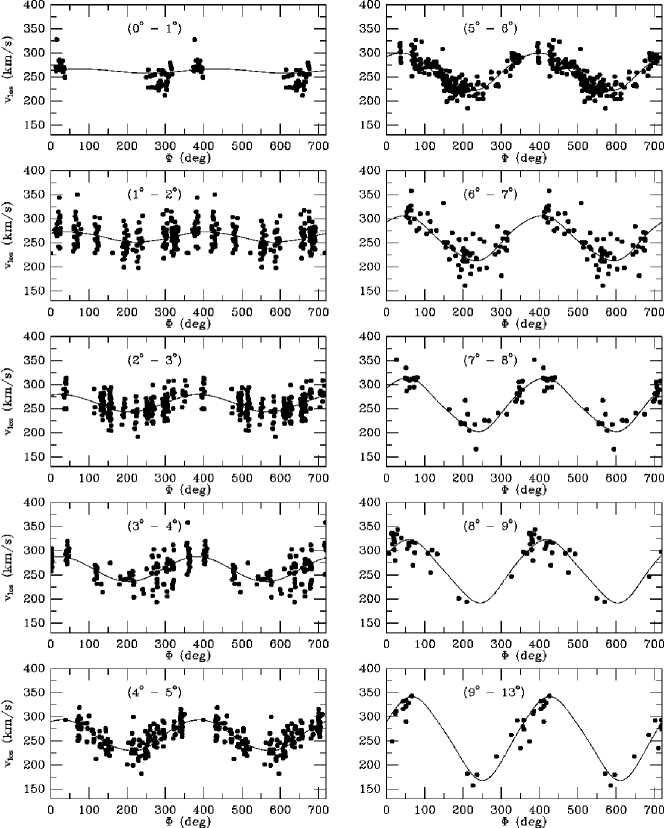
Figure 5: Carbon star line-of-sight velocity data from Kunkel et al. (1997) and Hardy et al. (2002, in prep.), as function of position angle $\Phi$ on the sky. The displayed range of the angle $\Phi$ is $0^{\circ}$–$720^{\circ}$, so each star is plotted twice. Each panel corresponds to a different range of angular distances $\rho$ from the LMC center, as indicated. The curves show the predictions of the best-fit model (calculated at the center of the radial range for the given panel).

The data and the best-fitting model are shown in Figure 5. For all radii $1^{\circ}\leq\rho\leq 9^{\circ}$ the fit is about as good as could be expected. At small radii, $\rho\leq 1^{\circ}$, there appears to be some systematic discrepancy between the data and the model. However, the data in the central degree (top left panel of Figure 5) provide too sparse coverage of the full range of position angles to draw any conclusions from this. There also appear to be minor discrepancies in the data-model comparison at radii $\rho\geq 9^{\circ}$. This could be due to tidal distortions in the LMC disk and its velocity field at large radii. Either way, these discrepancies do not affect the primary results of this paper in any significant way; fits to restricted radial ranges yielded identical results.

The right ascension $\alpha$ and declination $\delta$ of the CM and the parameters $v_{\rm sys}$, $w_{ts}$ and $\Theta$ are all determined unambiguously. The RMS residual of the fit is the (globally averaged) line-of-sight velocity dispersion $\sigma$ of the LMC. The model fit yields:

$$\alpha_{\rm CM} = 5^{\rm h}\>27.6^{\rm m}\>\pm 3.9^{\rm m}\>,$$

$$\delta_{\rm CM} = -69.87^{\circ}\pm 0.41^{\circ},$$

$$v_{\rm sys} = 262.2\pm 3.4\>{\rm km}\,{\rm s}^{-1},$$

$$w_{ts} = -402.9\pm 13.0\>{\rm km}\,{\rm s}^{-1},$$

$$\Theta = 129.9^{\circ}\pm 6.0^{\circ},$$

$$\sigma = 20.2\pm 0.5\>{\rm km}\,{\rm s}^{-1},$$ (53)

where the CM position is given in J2000.0 coordinates.

As discussed in Section 3, the quantity $v_{tc}$ and the rotation curve $V(R^{\prime})$ are not uniquely determined by the line-of-sight velocity field. The parameterized model that best fits the data has $v_{tc}=599\>{\rm km}\,{\rm s}^{-1}$ and the rotation curve $V(R^{\prime})$ that is shown as a solid curve in Figure 6. However, every other $v_{tc}$ will provide an equally acceptable fit, provided that $V(R^{\prime})$ is modified according to equation (50). The alternative rotation curves thus obtained are shown as dashed curves in Figure 6 for several values of $v_{tc}$. The value of $v_{tc}$ is constrained by the line-of-sight velocity field only through the fact that some of the rotation curves $V(R^{\prime})$ needed to fit the data are unplausible. If $v_{tc}$ is high, then $V(R^{\prime})$ is implausibly large for a low-luminosity galaxy such as the LMC. The LMC is slightly fainter than M33, $M_{V}=-18.5$ vs. $M_{V}=-18.9$, respectively (van den Bergh 2000), and the LMC and M33 have similar disk scale lengths (Paper II; Regan & Vogel 1994). According to the Tully-Fisher relation, the circular velocity of the LMC should be lower than for M33. For M33, $V(R^{\prime})\approx 120\>{\rm km}\,{\rm s}^{-1}$ at $R^{\prime}=11.6\>{\rm kpc}$ (Corbelli & Salucci 2000), the largest radius included in our study of the LMC. Figure 6 shows that for $v_{tc}=600\>{\rm km}\,{\rm s}^{-1}$, the LMC rotation curve levels off at $V(R^{\prime})\approx 130\>{\rm km}\,{\rm s}^{-1}$. This makes models with $v_{tc}\gtrsim 600\>{\rm km}\,{\rm s}^{-1}$ quite implausible. On the other hand, if $v_{tc}$ is low, less than $\sim 200\>{\rm km}\,{\rm s}^{-1}$, then $V(R^{\prime})$ has a sign change within the radial range out to which its starlight can be traced. This is never observed in disk galaxies. Based on these considerations we conclude that

$$v_{tc}\>\in\>[200,600]\>{\rm km}\,{\rm s}^{-1}.$$ (54)

The results described in this section were found to be very robust. We experimented with fits to subsets of the data, fits over restricted radial ranges, fits with different parameterizations for $V(R^{\prime})$, and different algorithms for the determination of the parameters that characterize the velocity field. All of this yielded results that are statistically equivalent to those described above.

5 The Proper Motion and Distance of the LMC

The analysis of the LMC line-of-sight velocity field has provided constraints on the velocities $v_{tc}$ and $w_{ts}$ (eqs. [4] and [54]). These velocities are directly related to the proper motion vector $(\mu_{W},\mu_{N})$ and distance $D_{0}$ of the LMC CM through equations (43), (44) and (45). To make further progress it is therefore useful to review what is already know about these quantities.

5.1 Proper Motion

Table 1 lists the proper motion measurements that are available for the LMC. They are from the following sources: Kroupa et al. (1994), using stars from the PPM Catalogue; Jones et al. (1994), using photographic plates with a 14 year epoch span; Kroupa & Bastian (1997), using Hipparcos data; Drake et al. (2002), using data from the MACHO project; and Pedreros et al. (2002), using CCD frames with an 11 year epoch span. The measurements of Jones et al. (1994) and Pedreros et al. (2002) pertain to fields in the outer parts in the LMC disk. These measurements require corrections for the orientation and rotation of the LMC disk. The proper motions listed in the table are based on the corrections that we derive in Appendix A, which are more accurate than the corrections derived in the original papers. The table does not include the measurement published by Anguita, Loyola & Pedreros (2000). Their result for the proper motion in the declination direction ($\mu_{N}=2.9\pm 0.2\>{\rm mas}\,{\rm yr}^{-1}$) is highly ($10\sigma$) inconsistent with all other studies. This probably indicates that the measurement contains some unidentified error; see Pedreros et al. (2002) and Drake et al. (2002) for some discussion of this issue.

Figure 7 shows the data from Table 1 in the $(\mu_{W},\mu_{N})$ plane. The ellipses around the data points indicate the corresponding 68.3% confidence regions. The proper motion measurements are in fair agreement with each other, in the sense that they fall in the same part of the diagram. The weighted average of the proper motion measurements in Table 1 is

$$\mu_{W}=-1.68\pm 0.16\>{\rm mas}\,{\rm yr}^{-1},\qquad\mu_{N}=0.34\pm 0.16\>{\rm mas}\,{\rm yr}^{-1}.$$ (55)

This is the LMC proper motion that we will use in the subsequent discussion. The corresponding 68.3% confidence region is indicated in Figure 7 by a heavy ellipse.

5.2 Distance

The distance $D_{0}$ to the LMC is a very important quantity in the calibration of the cosmological distance ladder. Most of the methods that are customarily used to study the Hubble constant of the Universe are ultimately calibrated by the distance to the LMC. The period-luminosity relation of Cepheids provides the most important, but by no means the only example. Of course, there now exist methods that provide information on the Hubble constant without requiring knowledge of the distance to the LMC. These use, e.g., gravitational lensing, the Sunyaev-Zeldovich effect, or the Cosmic Microwave Background radiation. However, the systematic uncertainties in these methods have not yet been reduced to levels where they can replace the more traditional techniques. The distance to the LMC therefore remains a topic of intense interest and debate in modern astronomy.

Many techniques have been used to estimate the LMC distance. Unfortunately, there continue to be systematic differences between the results from different techniques that exceed the formal errors. It is beyond the scope of the present paper to review this topic in detail. Instead, we refer the reader to the recent reviews by, e.g., Westerlund (1997), Gibson et al. (2000) and Freedman et al. (2001). Here we follow Freedman et al. by adopting

$$m-M=18.50\pm 0.10$$ (56)

for the LMC distance modulus, where $m-M\equiv 5\log(D_{0}/\>{\rm kpc})+10$. The implied distance is $D_{0}=50.1\pm 2.5\>{\rm kpc}$. At this distance, a proper motion of $1\>{\rm mas}\,{\rm yr}^{-1}$ corresponds to $238\pm 12\>{\rm km}\,{\rm s}^{-1}$ (eq. [10]), and 1 degree on the sky corresponds to $0.875\pm 0.044\>{\rm kpc}$.

New and improved distance determinations for the LMC continue to become available at a rapid rate. Recent measurements that were not yet included in the compilation of Freedman et al. (2001) include, e.g., measurements using the Tip of the Red Giant Branch (Cioni et al. 2000), eclipsing binaries (Fitzpatrick et al. 2002), RR Lyrae variables (Benedict et al. 2002) and the Red Clump (Alves et al. 2002, in prep.). The results from these recent studies are all consistent with the value adopted in equation (56).

6 Precession and Nutation of the LMC Disk

Equation (45) can be solved for $di/dt$ to obtain

$$di/dt=(w_{ts}/D_{0})-\mu_{s}.$$ (57)

The quantity $w_{ts}$ is determined by the line-of-sight velocity field, as is the line-of-nodes position angle $\Theta$ (eq.[4]). The proper motion component $\mu_{s}$ is determined by the literature average in equation (55), with help of the definition in equation (43). The distance is given by the literature average in equation (56). The rate of inclination change $di/dt$ is therefore uniquely determined by the available data. Evaluation of equation (57) yields

$$di/dt=-0.37\pm 0.22\>{\rm mas}\,{\rm yr}^{-1}=-103\pm 61\>\>{\rm degrees}/\>{\rm Gyr},$$ (58)

where a simple Monte-Carlo scheme was used for propagation of errors.

The LMC is the first galaxy for which it has been possible to measure $di/dt$. It is therefore useful to ask whether the inferred value is plausible, given our understanding of the LMC and its orbit around the Milky Way. Weinberg (2000) performed $N$-body simulations to assess the influence of the Milky Way on the structure and dynamics of the LMC. He found that the tidal torques from the Milky Way are expected to induce precession and nutation in the symmetry axis of the LMC disk plane. His figures 3 and 4 show the variations in the directions of the LMC symmetry axis for a generic simulation of the LMC (i.e., not fine-tuned to reproduce all the currently observed features of the LMC). On average, the rate of directional change in the three-dimensional angle is $\sim 60^{\circ}/\>{\rm Gyr}$ (i.e., $0.22\>{\rm mas}\,{\rm yr}^{-1}$). However, there are considerable variations with time, and at certain times the rate is several times larger. Whether this directional change is seen by an observer as a change in inclination or as a change in the line-of-nodes position angle depends on the exact location of the observer. Either way, the observed rate $di/dt$ given by equation (58) has the same order of magnitude as the generic predictions by Weinberg (2000). We therefore interpret the observed $di/dt$ as an indication of precession and nutation induced by tidal torques from the Milky Way.

The line-of-sight velocity field does not determine the second derivative $d^{2}i/dt^{2}$. It also does not provide any information on time variations in the position angle $\Theta$ of the line of nodes. It is therefore not possible to calculate either the past or the future variation of the orientation of the LMC symmetry axis in an inertial frame tied to the Milky Way. If one assumes that $d^{2}i/dt^{2}$ is always equal to zero, then the LMC would make one revolution every $3.5\pm 2.1\>{\rm Gyr}$. However, this number provides no real insight. The simulations of Weinberg show that LMC symmetry axis is expected to undergo nutation (i.e., oscillation with $d^{2}i/dt^{2}\not=0$) and not tumbling motion (i.e., full revolutions).

7 Kinematical Properties of the LMC disk

7.1 Dynamical Center

Previous authors who have modeled the dynamics of tracers in the LMC have fixed the dynamical center a priori, generally to coincide with the kinematical center of the HI gas. Kim et al. (1998) find this HI kinematical center to be at $\alpha=5^{\rm h}\>17.6^{\rm m}\>$ and $\delta=-69^{\circ}1^{\prime}$ (J2000.0 coordinates), with an accuracy that is probably better than $\sim 0.2^{\circ}$ in each coordinate. It has been a well-known result for many years that this position differs by almost a full degree from the center of the LMC bar (e.g., Westerlund 1997). The data from 2MASS yield for the latter $\alpha=5^{\rm h}\>25.1^{\rm m}\>\pm 0.1^{\rm m}\>$ and $\delta=-69^{\circ}47^{\prime}\pm 1^{\prime}$ (Paper II). Our analysis in Section 4 is the first to provide an accurate measurement of the dynamical center of the stars in the LMC, by leaving it as a completely free parameter in the fit. We obtain $\alpha_{\rm CM}=5^{\rm h}\>27.6^{\rm m}\>\pm 3.9^{\rm m}\>$ and $\delta_{\rm CM}=-69^{\circ}52^{\prime}\pm 25^{\prime}$ (eq. [4]). This is consistent with the position of the center of the bar. It is also consistent with the position of the center of the outer isophotes of the LMC (corrected for the effect of viewing perspective), which is at approximately $\alpha=5^{\rm h}\>29^{\rm m}\>$ and $\delta=-69^{\circ}30^{\prime}$ (Paper II). However, the dynamical center of the stars differs from the dynamical center of the gas by as much as $1.2^{\circ}\pm 0.6^{\circ}$. These results suggest that the gas kinematics are quite disturbed, while the stellar kinematics show little evidence for peculiar behavior. This is not particularly surprising in view of other knowledge about the gas in the Magellanic Clouds, which is quite disturbed in general (witness the Magellanic Bridge and the Magellanic Stream). These results make it unlikely that any study of the HI in the LMC will ever lead to an accurate understanding of its structure and dynamics.

7.2 Rotation Curve

For studies of the dynamics and mass distribution of the LMC it is useful to have an unparameterized description of its rotation and velocity dispersion profiles. To this end we have performed fits of the velocity field given by equation (40) to individual rings in the plane of the LMC disk. The rotation velocity $V(R^{\prime})$ and the line of sight position angle $\Theta$ were assumed to be constant over each ring, and were determined so as to best fit the data. The resulting kinematical profiles are listed in Table 2, and are shown in Figure 6. In the fits we kept the quantities $(\alpha_{\rm CM},\delta_{\rm CM},v_{\rm sys},w_{ts},i)$ fixed to their previously determined values (eqs. [51] and [4]). The value of $v_{tc}$ was fixed to that implied by the LMC proper motion; from equations (43, 44, 4, 55, 56) one obtains

$$v_{tc}=253\pm 52\>{\rm km}\,{\rm s}^{-1}.$$ (59)

This is not inconsistent with the weak constraint $v_{tc}\>\in\>[200,600]\>{\rm km}\,{\rm s}^{-1}$ that was obtained from the analysis of the line-of-sight velocity field (eq. [54]).

The inferred rotation curve $V(R^{\prime})$ rises linearly in the central region and is roughly flat at $V\approx 50\>{\rm km}\,{\rm s}^{-1}$ for $R^{\prime}\gtrsim 4\>{\rm kpc}$ (i.e., $R^{\prime}/D_{0}\gtrsim 0.08$). The error bars in $V(R^{\prime})$ do not take into account the errors in $(\alpha_{\rm CM},\delta_{\rm CM},v_{\rm sys},w_{ts},i,v_{tc})$, which were all kept fixed. In reality, the errors in $i$ and $v_{tc}$ do add additional uncertainty to the rotation curve. The uncertainty in $i$ (eq. [51]) causes a $\sim 15$% uncertainty in the normalization of $V(R^{\prime})$, cf. equation (50). No other part of our analysis depends on the exact choice of the inclination. The influence of the $52\>{\rm km}\,{\rm s}^{-1}$ error in $v_{tc}$ (eq. [59]) can be assessed visually from Figure 6.

The innermost data point in Figure 6 at $R^{\prime}/D_{0}\approx 0.01$ (i.e., $R^{\prime}\approx 0.5\>{\rm kpc}$) is clearly discrepant from the data points at larger radii, both in terms of its kinematic position angle $\Theta$ and its rotation velocity $V$. Although this could be attributed to non-circular streaming motions in the region of the bar, this result has only very low significance. The top left panel of Figure 5 shows that the data in this region provide only very sparse coverage of the full range of position angles. Better data are needed to address the kinematics in the central kpc with any confidence.

Alves & Nelson (2000) previously analyzed the carbon-star kinematics of the LMC. Like most authors, they didn’t use the fully correct expression for the velocity field of a rotating disk at finite distance (last term in eq. [40]) and they assumed $di/dt=0$. They corrected for the transverse motion of the LMC using an assumed proper motion $(\mu_{W},\mu_{N})=(-1.65\pm 0.20,-0.17\pm 0.22)\>{\rm mas}\,{\rm yr}^{-1}$. This is an average of the proper motion measurements by Jones et al. (1994) and Kroupa & Bastian (1997). This proper motion, combined with $di/dt=0$, implies $v_{tc}=325\pm 57\>{\rm km}\,{\rm s}^{-1}$ and $w_{ts}=-220\pm 62\>{\rm km}\,{\rm s}^{-1}$ (cf. eqs.[43, 44, 4, 55, 56). The value of $w_{ts}$ is quite different from the value that we have obtained here from a fit to the velocity field, $w_{ts}=-402.9\pm 13.0\>{\rm km}\,{\rm s}^{-1}$ (cf. eq. [4]). The result of enforcing an incorrect value of $w_{ts}$ on the solution is that one obtains an incorrect value for the position angle of the line of nodes. Alves & Nelson obtained a kinematic line of nodes that is both twisting and inconsistent with the geometrically determined line of nodes (see Section 1). Since the rotation curve is determined by the velocities measured along the line of nodes, one also obtains an incorrect estimate of the rotation curve. Alves & Nelson obtained a rotation curve amplitude of $\sim 70\>{\rm km}\,{\rm s}^{-1}$, which exceeds ours by $\sim 40$%.

The analysis by Kim et al. (1998) of the HI velocity field suffered from similar shortcomings. They corrected for the transverse motion of the LMC using the proper motion advocated by Jones et al. (1994), $(\mu_{W},\mu_{N})=(-1.37\pm 0.28,-0.18\pm 0.27)\>{\rm mas}\,{\rm yr}^{-1}$. This proper motion, combined with $di/dt=0$, implies $v_{tc}=276\pm 69\>{\rm km}\,{\rm s}^{-1}$ and $w_{ts}=-175\pm 72\>{\rm km}\,{\rm s}^{-1}$. Again, the value of $w_{ts}$ is quite different from the value that we have obtained here from a fit to the velocity field. So, like Alves & Nelson, Kim et al. obtained a kinematic line of nodes that is both twisting and inconsistent with the geometrically determined line of nodes, as well as a rotation curve amplitude that exceed ours by $\sim 40$%.

7.3 Velocity Dispersion Profile

The velocity dispersion profile that we derive for the carbon stars in the LMC is shown in the middle panel of Figure 6. It is not very different from the velocity dispersion profile derived by Alves & Nelson (2000). The dispersion is 20–$22\>{\rm km}\,{\rm s}^{-1}$ between $1$ and $3.5\>{\rm kpc}$ from the center, followed by a decline to 16–$17\>{\rm km}\,{\rm s}^{-1}$ between $3.5$ and $7\>{\rm kpc}$ from the center, and a subsequent increase to 21–$22\>{\rm km}\,{\rm s}^{-1}$ between $7$ and $9\>{\rm kpc}$.

The different stellar populations in the LMC are not characterized by a single velocity dispersion. As in the Milky Way, younger populations have a smaller velocity dispersion than older populations. A summary of measurements for various populations is given by Gyuk, Dalal & Griest (2000). They range from $\sigma\approx 6\>{\rm km}\,{\rm s}^{-1}$ for the youngest populations (e.g., supergiants, HII regions, HI gas) to $\sigma\approx 30\>{\rm km}\,{\rm s}^{-1}$ for the oldest populations (e.g., old long-period variables, old clusters). Any discussions in the remainder of the paper that use our velocity dispersion measurements, e.g., those in Section 8.3 concerning the LMC scale height, apply strictly only to carbon stars. On the other hand, the carbon stars are part of the intermediate-age population which is believed to be fairly representative for the bulk of the mass in the LMC. In this sense, the results inferred for the carbon star population are believed to be generic for the LMC as a whole.

7.4 Line of Nodes Position Angle

The fit to the velocity field described in Section 4 implies a line-of-nodes position angle $\Theta=129.9^{\circ}\pm 6.0^{\circ}$ (eq. [4]). This agrees within the errors with the geometrically determined line-of-nodes position angle, $\Theta=122.5\pm 8.3^{\circ}$ (Paper I). This agreement was not in any way built into the model, and it therefore provides an important consistency check on the validity of our approach. This is particularly important because it resolves the discrepancy that emerged from previous kinematical analyses of the LMC (see Section 1). It also provides further confirmation of the finding from Paper II that the position angle of the line nodes is very different from the position angle of the LMC major axis (${\rm PA}_{\rm maj}=189.3^{\circ}\pm 1.4^{\circ}$), and hence that the LMC is not intrinsically circular.

The bottom panel of Figure 6 shows that the radial profile of $\Theta$ is approximately flat (with the exception of the innermost point, which has very low significance; see Section 7.2). The constancy of $\Theta$ as a function of radius should come as no surprise. Our velocity field model does not allow for radial twists in $\Theta$. The best-fitting value for $w_{ts}$ is therefore, by definition, the value that yields the least possible radial variation in $\Theta$. One might wonder if this is not the equivalent of forcing a square peg into a round hole. After all, the projected morphology of the LMC shows a considerable isophotal twist between the region of the bar and the outer parts of the disk (Paper II). While this is certainly a worry, we have found little evidence that there is a corresponding twist in the kinematic line of nodes. First, the results of the present paper, which assume an absence of kinematic twists, provide a highly consistent view of the LMC. Second, there is no evidence for any isophotal twist at projected radii $\rho\geq 4.5^{\circ}$, suggesting that at least at these radii there are probably no twists in the kinematic line of nodes. Kinematical fits restricted to the range $\rho\geq 4.5^{\circ}$ yielded results that were statistically consistent with those for the full radial range.

7.5 Influence of Non-Circular Streamlines

It was shown in Paper II that the LMC is not intrinsically circular, but instead has an ellipticity $\epsilon=1-(b/a)=0.31\pm 0.01$. However, the gravitational potential of a mass distribution is always rounder than the mass distribution, which provides some a priori justification for the use of a model in which the streamlines are circular. There is also some a posteriori justification from the fact that the kinematically inferred position angle of the line of nodes, $\Theta_{\rm kin}=129.9^{\circ}\pm 6.0^{\circ}$ (eq. [4]), agrees with the geometrically determined value, $\Theta=122.5\pm 8.3^{\circ}$ (Paper I). Detailed dynamical models of elliptical disks generally predict a (small) misalignment between $\Theta_{\rm kin}$ and $\Theta$ (e.g., Schoenmakers, Franx & de Zeeuw 1997). The fact that no such misalignment is detectable with the available statistics ($\Theta_{\rm kin}-\Theta=7.4^{\circ}\pm 10.2^{\circ}$) suggests that a model with circular streamlines may not be unreasonable in the present context. Note, however, that this argument cannot be reversed. The fact that $\Theta_{\rm kin}-\Theta$ is small does not by itself imply that the streamlines must be nearly circular (Jalali & Abolghasemi 2002).

Unfortunately, there are no unambiguous theoretical methods for calculating the velocity field of an elliptical disk. Some results have been obtained for gaseous systems (Jalali & Abolghasemi 2002), but stellar systems are more complicated because they can have an anisotropic velocity dispersion (i.e., pressure) tensor. It is therefore difficult to estimate the systematic errors in our results due to the simplifying assumption of circular streamlines. It should be noted though, that even if the streamlines are not circular, this will not invalidate our approach at a basic level. Even in an elliptical disk there is generally a position angle $\Upsilon$ along which the line-of-sight velocity component is zero (Schoenmakers et al. 1997). Unlike in a circular disk, one will not generally have that $\Upsilon=\Theta+90^{\circ}$, where $\Theta$ is the true geometrical line of nodes. However, along the position angle $\Upsilon$ one still has that ${\hat{v}}_{\rm los}=\pm w_{ts}\sin\rho$, as in equation (49). So for an elliptical disk one can still, at least in principle, constrain $\Upsilon$ and $w_{ts}$ from the line-of-sight velocity field. However, the actual algorithm employed here will not be quite sufficient to yield highly accurate results. We rely on fitting the velocity field given by equation (40), which for an elliptical disk is not generally valid at all position angles $\Phi$. It is not clear how important this is for the present analysis, but it will certainly become more important as larger samples of carbon star line-of-sight velocities will become available in the future. This will decrease the formal error random errors in the modeling, at which point deviations from circular streamlines may start to play a more important role.

8 Structure of the LMC Disk

An important result of the present study is that we find the rotation curve amplitude of the LMC to be $\sim 40$% lower than suggested on the basis of previous analyses (see Section 7.2). This changes our understanding of several important structural parameters and properties of the LMC.

8.1 Mass

Figure 6 shows that the rotation curve of the LMC is approximately flat from $R\approx 4\>{\rm kpc}$ out to the last data point at $R=8.9\>{\rm kpc}$. The weighted mean of the rotation velocity data points in this radial range is $V=49.8\>{\rm km}\,{\rm s}^{-1}$. There are several uncertainties in this rotation curve amplitude: (i) an error of $\pm 2.1\>{\rm km}\,{\rm s}^{-1}$ due to the finite number of data points; (ii) an error of $\pm 7.8\>{\rm km}\,{\rm s}^{-1}$ due to the error in our knowledge of the LMC inclination (eq. [51]); and most importantly (iii) an error of approximately $\pm 13.7\>{\rm km}\,{\rm s}^{-1}$ due the error in our knowledge of $v_{tc}$ (eq. [59] and Figure 6). Addition of these errors in quadrature yields $V=49.8\pm 15.9\>{\rm km}\,{\rm s}^{-1}$. The weighted mean line-of-sight velocity dispersion over the same radial range is $\sigma=16.9\pm 0.5\>{\rm km}\,{\rm s}^{-1}$.

Due to asymmetric drift, the average azimuthal streaming velocity $V$ is always smaller than the velocity $V_{\rm circ}$ of a tracer on a circular orbit in the equatorial plane. For the solar neighborhood in the Milky Way, observations indicate that $V_{\rm circ}^{2}\approx V^{2}+5.5\sigma_{R}^{2}$ (Dehnen & Binney 1998). For the LMC we expect similarly that $V_{\rm circ}^{2}=V^{2}+\kappa\sigma^{2}$, where $\sigma$ is the observed line-of-sight velocity dispersion and $\kappa$ is a model dependent factor. Since the formal error in $V$ is quite large, there is no particular benefit in making very sophisticated models to determine $\kappa$. A simple model that is adequate in the present context considers the equatorial plane of an axisymmetric system with an isotropic velocity distribution embedded in an isothermal dark halo. The equations of van der Marel (1991) then show that $-\kappa$ is equal to the logarithmic slope of the mass density in the equatorial plane. For an exponential disk this yields $\kappa=R/R_{d}$, where $R_{d}$ is the exponential disk scale length. From Paper II we know that the LMC is modestly well described by an exponential profile with $R_{d}\approx 1.5\>{\rm kpc}$. This implies that at the last measured data point $\kappa\approx 6$ and $V_{\rm circ}=64.8\pm 15.9\>{\rm km}\,{\rm s}^{-1}$ (the error on $V_{\rm circ}$ does not include a theoretical error on $\kappa$, given that its influence would most likely be negligible compared to the formal error in $V$).

The total mass of the LMC inside the last measured data point is $M_{\rm LMC}(R)=RV_{\rm circ}^{2}/G$, where the gravitational constant $G=4.3007\times 10^{-6}\>{\rm kpc}(\>{\rm km}\,{\rm s}^{-1})^{2}\>{\rm M_{\odot}}^{-1}$. This yields $M_{\rm LMC}(8.9\>{\rm kpc})=(8.7\pm 4.3)\times 10^{9}\>{\rm M_{\odot}}$. Despite its relatively large error bar, our estimate is considerably more accurate in a systematic sense than the results of previous studies. Nonetheless, we find that (after correction for the fact that different authors tend to quote masses enclosed within different radii) our result is similar to most other LMC mass estimates in the literature (e.g., Feitzinger et al. 1977; Meatheringham et al. 1988; Kim et al. 1998). The reason for this is that while previous authors generally inferred a higher rotation curve amplitude $V$ (see Section 7.2), their general neglect of the asymmetric drift correction led to similar estimates of $V_{\rm circ}$. Our mass estimate does differ considerably from that presented by Schommer et al. (1992). They applied a statistical mass estimator to the velocities of a sample of 16 old LMC clusters to infer a mass $M_{\rm LMC}\approx 2\times 10^{10}\>{\rm M_{\odot}}$ within an effective radius of $\sim 6\>{\rm kpc}$. This result is inconsistent with the analysis presented here. Several $N$-body simulation studies of the LMC have assumed, following Schommer et al. , that $\sim 2\times 10^{10}\>{\rm M_{\odot}}$ is enclosed inside the visible body of the LMC (e.g., Gardiner, Sawa & Fujimoto 1994; Gardiner & Noguchi 1996; Weinberg 2000). It is likely that these simulations have overestimated the self-gravity of the LMC compared to the Milky Way tidal force.

8.2 Tidal Radius

To calculate the tidal radius of the LMC we consider the gravitational accelerations at a point on the line that connects the Milky Way to the LMC. Let the point be at a distance $\beta D_{0}$ from the LMC center and at a distance $[1-\beta]D_{0}$ from the Milky Way center. We assume that $\beta\ll 1$; the calculations can easily be carried out to full accuracy, but this does not lead to significantly different results. Let ${\vec{a}}_{\rm MW}$ be the gravitational acceleration due to the Milky Way and ${\vec{a}}_{\rm LMC}$ the gravitational acceleration due to the LMC. The tidal radius corresponds to the point at which ${\vec{a}}_{\rm MW}([1-\beta]D_{0})-{\vec{a}}_{\rm MW}(D_{0})=-{\vec{a}}_{\rm LMC}(\beta D_{0})$.

The traditional assumption in the calculation of the tidal radius is that both bodies can be approximated to be point masses. In this case one obtains that

$$\beta_{\rm tidal}\equiv\beta_{1}=[M_{\rm LMC}/2M_{\rm MW}]^{1/3}.$$ (60)

This equation was used, e.g., by Weinberg (2000; his appendix A). However, this equation is not really appropriate, because there is strong evidence that the mass of the Milky Way continues to rise linearly to beyond the distance of the LMC (e.g., Kochanek 1996; Wilkinson & Evans 1999). If one assumes instead that the Milky Way has a flat rotation curve with circular velocity $V_{0}$, while still assuming that the LMC is a point mass, then

$$\beta_{\rm tidal}\equiv\beta_{2}=[M_{\rm LMC}/M_{\rm MW}(D_{0})]^{1/3}.$$ (61)

where $M_{\rm MW}(D_{0})$ is the mass of the Milky Way inside a sphere of radius $D_{0}$. This yields a tidal radius that is a factor $2^{1/3}=1.26$ larger than the value given by equation (60). If one assumes that the LMC itself can also not be approximated as a point mass, but instead has a constant circular velocity $V_{\rm circ}$ (i.e., mass rising linearly with radius), then

$$\beta_{\rm tidal}\equiv\beta_{3}=V_{\rm circ}/V_{0}.$$ (62)

The kinematical data that are available for the LMC do not extend as far out as the tidal radius, so we do not know whether the LMC circular velocity curve at the tidal radius is flat or Keplerian. The LMC tidal radius, $r_{t}\equiv\beta_{\rm tidal}D_{0}$, must therefore be in the range $\beta_{2}D_{0}\lesssim r_{t}\lesssim\beta_{3}D_{0}$. To evaluate equation (61) we use $M_{\rm LMC}=(8.7\pm 4.3)\times 10^{9}\>{\rm M_{\odot}}$ from Section 8.1 and $M_{\rm MW}(D_{0})=(4.9\pm 1.1)\times 10^{11}\>{\rm M_{\odot}}$ from Kochanek (1996), which yields $\beta_{2}=0.26\pm 0.05$. To evaluate equation (62) we use $V_{\rm circ}=64.8\pm 15.9\>{\rm km}\,{\rm s}^{-1}$ from Section 8.1 and $V_{0}=206\pm 23\>{\rm km}\,{\rm s}^{-1}$ based on the mass given by Kochanek, which yields $\beta_{3}=0.31\pm 0.08$. We combine these results to obtain for the LMC tidal radius that $r_{t}=15.0\pm 4.5\>{\rm kpc}$. This corresponds to an angle on the sky of $17.1^{\circ}\pm 5.1^{\circ}$.

The result thus calculated can be compared to our observational knowledge of the outer parts of the LMC. Data from the 2MASS survey show that the isopleths of RGB and AGB stars can be traced out to a major axis radius of $\sim 9^{\circ}$ and are regular out to this radius (Paper II). APM measurements of photographic Schmidt plates have revealed regular isopleths out to $\sim 11.5^{\circ}$ (Irwin 1991). Observations therefore indicate that $r_{t}\gtrsim 11.5^{\circ}$, consistent with value calculated above. Having said this, it must be kept in mind that the tidal radius is not a particularly well-defined quantity, especially not for a disk system such as the LMC. The Milky Way center does not lie in the plane of the LMC disk (Paper II). As a consequence, for points in the LMC disk the gravitational accelerations ${\vec{a}}_{\rm MW}$ and ${\vec{a}}_{\rm LMC}$ are not colinear. So there is no radius in the disk where they add up to zero. Also, as the LMC orbits the Milky Way, the angle between the acceleration vectors changes. The effect of the Milky Way tidal force therefore need not lead to a sharp truncation of the disk, but instead may lead to thickening of the disk and the formation of an extended halo of unbound particles (Weinberg 2000).

8.3 Scale Height

The observed velocity dispersion profile contains important information on the scale height of the LMC as function of radius, as discussed in detail by Alves & Nelson (2000). They found that the velocity dispersion profile does not fall steeply enough with radius to be consistent with a constant scale-height disk. From this they concluded that the disk must be ‘flared’, with a scale height that increases radially outward. This can arise naturally as a result of tidal forces from the Milky Way. These forces become relatively more important (compared to the LMC self-gravity) as one moves to larger radii. Indeed, the $N$-body simulations by Weinberg (2000) predict a considerable thickness for the LMC disk as a result of the Milky Way tidal forces (although, somewhat surprisingly, the vertical velocity dispersion in his simulations remains small).

It is straightforward to refit the isothermal flared disk model of Alves & Nelson (2000; their eq. [37]) to our new kinematical results and preferred LMC disk parameters. For an isothermal disk the vertical density profile is proportional to ${\rm sech}^{2}(z/z_{0})$, where $z_{0}$ can vary with disk radius. The input to the model of Alves & Nelson (2000) includes the total disk mass (Section 8.1), the radial exponential scale length of the disk (Paper II), the total mass of the LMC dark halo (Section 8.4), the mean density of the Milky Way’s dark halo at the LMC distance (Section 9.4) and approximate corrections for the finite thickness and finite radial extent of the disk. The best fit to our velocity dispersion data (Figure 6 and Table 2) yields $z_{0}=0.27\>{\rm kpc}$ at the LMC center, rising to $z_{0}=1.5\>{\rm kpc}$ at a radius of $5.5\>{\rm kpc}$. If one prefers to model the disk’s thickness with an exponential instead of a ${\rm sech}^{2}$ function, then the exponential scale height is approximately half of $z_{0}$ (Gilmore, King & van der Kruit 1990).

It is useful to compare the LMC disk to the disk components of our Milky Way galaxy. The thin disk of the Milky Way has $V/\sigma\approx 9.8$ and the thick disk has $V/\sigma\approx 3.9$. For the LMC we have, averaged between $4$ and $9\>{\rm kpc}$ as in Section 8.1, that $V/\sigma\approx 2.9\pm 0.9$. The Milky Way thick disk has an exponential vertical scale height $z_{d}\approx 1\>{\rm kpc}$ (Binney & Merrifield 1998). Its exponential radial scale length is $R_{d}\approx 3\>{\rm kpc}$, if one assumes that the Milky Way thin and thick disks have the same radial profile. Hence, at the solar radius ($\sim 3R_{d}$), the Milky Way thick disk is characterized by a relative thickness $z_{d}/R_{d}\approx 1/3$. This is quantitatively similar to the values inferred for the LMC, upon application of Alves & Nelson’s (2000) flared disk model to our new data. At $3R_{d}\approx 4.5\>{\rm kpc}$, the model predicts $z_{0}=1.1\>{\rm kpc}$. The corresponding exponential scale height (see above) is $z_{d}\approx 0.5\>{\rm kpc}$ so that $z_{d}/R_{d}\approx 1/3$. So both in terms of $V/\sigma$ as well as in terms of $z_{d}/R_{d}$, the LMC is very similar to the thick disk of the Milky Way and very different from the thin disk of the Milky Way.

There are different approaches to estimate the actual shape and vertical scale height of the LMC disk. A useful alternative to the approach employed by Alves & Nelson (2000) is to assume that the LMC is spheroidal with axial ratio $q$ (for reference, an infinitely thin disk has $q\ll 1$ whereas the very flattest elliptical galaxies have $q\approx 0.3$; Binney & Merrifield 1998). The axial ratio is directly related to the quantity $V/\sigma$ through hydrostatic equilibrium. For a self-gravitating system one can use the relation provided by the tensor virial theorem (Binney & Tremaine 1987). However, this relation is not accurate for the LMC, which is embedded in a dark halo (see Section 8.4 below). So we consider another simple model instead: we assume that the LMC is embedded in a spherical isothermal halo, and that it has an isotropic velocity dispersion that is approximately constant as function of radius. The equations of van der Marel (1991) then yield that

$$q=\left\{2+\left[{2\over\kappa}(V/\sigma)^{2})\right]\right\}^{-1/2},$$ (63)

where, as in Section 8.1, $-\kappa$ is the logarithmic slope of the mass density in the equatorial plane: $\kappa\approx R/R_{d}$ with $R_{d}\approx 1.5\>{\rm kpc}$. This simple model suggest that the axial ratio ranges from $q\approx 0.31$ at $R=3\>{\rm kpc}$ to $q\approx 0.46$ at $R=9\>{\rm kpc}$. These results are qualitatively consistent with those from Alves & Nelson’s (2000) flaring disk model.

The LMC has $V/\sigma$ considerably larger than unity, and it therefore remains quite justified to regard the LMC as a rotationally supported disk-like system. However, it is most definitely not a thin disk. Although the axial ratio values that we have estimated are based on simple models, and need to be interpreted with care, it is clear that the LMC is quite thick. While this does not appear to have been fully appreciated in the literature, it need not come as a surprise. The inferred thickness is entirely consistent with the predictions from simulations (Weinberg 2000).

8.4 Dark Halo

The total $B$-band magnitude of the LMC is $0.63$ (de Vaucouleurs & Freeman 1973), the $B-V$ color is $0.61\pm 0.03$ (Bothun & Thompson 1988), and the V-band extinction is $A_{V}\approx 0.4$ (Zaritsky 1999). This implies a total intrinsic luminosity $L_{V}=3.0\times 10^{9}\>{\rm L_{\odot}}$. Realistic stellar population synthesis and evolution models for disk galaxies predict a strong correlation between color and mass-to-light ratio. To fit the extinction-corrected $B-V$ color, the mass-to-light ratio of the stellar population should be $M/L_{V}\approx 0.9\pm 0.2$ (Bell & de Jong 2001), with some residual dependence on the assumed initial mass function and its low-mass cut-off. This implies a total mass for the visible disk of the LMC of $M\approx 2.7\times 10^{9}\>{\rm M_{\odot}}$. The mass of the neutral gas in the LMC has been estimated to be $0.5\times 10^{9}\>{\rm M_{\odot}}$ (Kim et al. 1998). The combined mass of the visible material in the LMC is therefore insufficient to explain the dynamically inferred mass $M_{\rm LMC}(8.9\>{\rm kpc})=(8.7\pm 4.3)\times 10^{9}\>{\rm M_{\odot}}$ (Section 8.1). Consequently, the LMC must be embedded in a dark halo. This is consistent also with the fact that the observed rotation curve amplitude is relatively flat as a function of radius. To determine the properties of the LMC dark halo one must: (i) model the contributions to the circular velocity from gas, stars and dark matter; (ii) calculate the asymmetric drift; (iii) perform a detailed data-model comparison. Such a detailed analysis is beyond the scope of the present paper. Alves & Nelson (2000) did perform such modeling, but their results will need to revised in view of the present paper: they used an observed rotation curve amplitude that is 40% higher than the one that we have inferred here, and they ignored asymmetric drift.

The observed rotation velocity $V(R)$ listed in Table 2 rises very slowly; it does not reach its flat part until $R\approx 4\>{\rm kpc}$. This is different from the behavior of the circular velocity curves $V_{\rm circ}(R)$ predicted by realistic models, which reach velocities near their maximum already at $R\approx 2\>{\rm kpc}$ (Alves & Nelson 2000). This indicates, independent of model details, that $V<V_{\rm circ}$ in the central region of the LMC. Our favored explanation for this is that it is the result of asymmetric drift. In the central $R\lesssim 2\>{\rm kpc}$, $V/\sigma$ is of order unity. We do not think that it is due to some error in the rotation curve $V(R)$ inferred from the observations. At small radii, $V(R)$ is rather insensitive to errors in $v_{tc}$, cf. Figure 6. There also is no strong dependence on the assumed position angle of the line of nodes. Alves (2000) also found that $V<V_{\rm circ}$ at $R\lesssim 4\>{\rm kpc}$, despite the use of a very different line of nodes position angle. Nonetheless, one must not forget that the central region of the LMC contains a strong bar. So it is quite likely that the streaming velocity field in this region is considerably more complicated than the circular streaming model that we have used in our analysis. A proper understanding of the kinematics and mass distribution of the LMC in its central few kpc will require detailed modeling of both bar dynamics and asymmetric drift.

8.5 Microlensing Optical Depth

The observed microlensing optical depth towards the LMC is $\tau_{\rm obs}=12^{+4}_{-3}\times 10^{-8}$ with an additional 20–30% of systematic error (Alcock et al. 2000). To interpret this result it is critically important to know the self-lensing optical depth of the LMC, $\tau_{\rm self}$. This subject was addressed and reviewed most recently by Gyuk et al. (2000). For their most favored set of LMC model parameters they predict $\tau_{\rm self}=2.2\times 10^{-8}$, a factor of $5.5$ less than the observed value. It is useful to address whether our new results on LMC structure change this conclusion.

To lowest order, the LMC self-lensing optical depth depends exclusively on the observed velocity dispersion and not separately on either the galaxy mass or scale height (Gould 1995). The values that we have inferred here for the line-of-sight velocity dispersion of the LMC are not very different from those used by previous authors. This argues that, to lowest order, our new findings do not change the predictions for the LMC self-lensing optical depth. In principle, the expression derived by Gould (1995) is somewhat idealized. It relies on the assumptions that: (a) the LMC disk is thin; and (b) the observed velocity dispersion tracks the scale height as in simple equilibrium models. The first assumption is suspect based on our discussion in Section 8.3 and the second assumption has been shown to be violated in the $N$-body simulations of Weinberg (2000). One could therefore argue that it is prudent to consider more sophisticated models. However, this was done by Gyuk et al. (2000), and they did not find results that differ greatly from the simple predictions obtained directly from the velocity dispersion. Alves & Nelson (2000) incorporated the flaring of the LMC disk, and this too was found not to increase $\tau_{\rm self}$ very significantly. The MACHO survey fields used to derive $\tau_{\rm obs}$ are mostly situated in the central 2 kpc of the LMC (Alcock et al. 2000), and at these radii the flaring is not yet substantial enough to make a big difference (see Section 8.3). In view of these arguments, it appears unlikely that the revised understanding of LMC structure that has emerged from the present study will significantly increase the predicted LMC self-lensing optical depth.

For LMC self-lensing models to become a viable explanation for the observed lensing events they will not only have to correctly predict $\tau_{\rm obs}$, but also the observed spatial and time-scale distributions of the lensing events (Gyuk et al. 2000; Alcock et al. 2000). Proposed tests of the lensing population based on the spatial distribution of the events may need to be revisited in light of our new and coherent understanding of LMC structure. For example, the tests discussed by Alcock et al. (2000; their section 5.3; see also Gyuk et al. 2000) are based on an incorrect line of nodes position angle of $170^{\circ}$. This is quite different from the actual value, which has now been found using several different methods to be in the range $120^{\circ}$–$130^{\circ}$ (Papers I and II; Section 4). This error could become important, particularly if larger samples of microlensing events become available. The flare of the LMC disk is also important for self-lensing models. It causes the spatial distribution to more resemble that expected for LMC halo lenses. The event rate will fall off more gradually with radius than if the disk had a constant thickness, and the near-to-far side event rate asymmetry will be less. It may be worth investigating new tests of the spatial event distribution that build on our improved understanding of the LMC structure (e.g., a test based on the event distance perpendicular to the line-of-nodes).

9 The Orbit of the LMC

9.1 Systemic Velocity

As mentioned in Section 4, the kinematical properties of the LMC have been studied previously using many different tracers. Each of these studies has yielded an estimate of the systemic velocity of the LMC. The result that has most often been adopted in models of the Milky Way dark halo and the Magellanic Stream (e.g., Wilkinson & Evans 1999; Gardiner et al. 1994) is the value $v_{\rm sys}=274\>{\rm km}\,{\rm s}^{-1}$ inferred from HI data by Luks & Rohlfs (1992). This value is similar to the value $v_{\rm sys}=279\>{\rm km}\,{\rm s}^{-1}$ inferred subsequently, also from HI data, by Kim et al. (1998). However, the HI distribution and kinematics in the LMC are quite disturbed. For example, Luks & Rohlfs required two separate HI velocity components to fit their data, and as discussed in Section 7.1, the HI dynamical center probably does not coincide with the LMC CM. The true systemic velocity, i.e., the line-of-sight velocity of the CM, is therefore better estimated from discrete tracers. From our analysis of 1041 carbon stars we have obtained $v_{\rm sys}=262.2\pm 3.4\>{\rm km}\,{\rm s}^{-1}$ (eq. [4]). The error in the determination of $v_{\rm sys}$ scales as $1/\sqrt{N}$, where $N$ is the number of tracers. Previous studies with other tracers generally had much smaller values of $N$ than available for the present study. For example, Meatheringham et al. (1988) studied 94 planetary nebulae; Schommer et al. (1992) studied 83 star clusters; etc. We conclude that our estimate of $v_{\rm sys}$ is the most accurate one currently available.

9.2 Transverse Velocity

The observed proper motion of the LMC quoted in equation (55) yields an estimate of the transverse velocity of the LMC. With the help of equations (44) and (56) one obtains

$$v_{x}=-399\>{\rm km}\,{\rm s}^{-1},\qquad v_{y}=80\>{\rm km}\,{\rm s}^{-1},$$ (64)

where the $x$ and $y$ directions point towards the West and North, respectively. This result corresponds to a velocity $v_{t}=406\>{\rm km}\,{\rm s}^{-1}$ in the direction of position angle $\Theta_{t}=78.7^{\circ}$. The uncertainty in the distance $D_{0}$ causes the error $\Delta v$ in the transverse velocity to be larger in the direction $\Theta_{t}$ than in the direction $\Theta_{t}+90^{\circ}$:

$$\Delta v(\Theta_{t})=44\>{\rm km}\,{\rm s}^{-1},\qquad\Delta v(\Theta_{t}+90^{\circ})=37\>{\rm km}\,{\rm s}^{-1}.$$ (65)

The $68.3$% confidence region on the transverse velocity of the LMC is shown as a heavy ellipse in Figure 8.

The analysis of the line-of-sight velocity field also constrains the transverse velocity of the LMC. This velocity is determined completely by the orthogonal components $v_{tc}$ and $v_{ts}$, measured along and perpendicular to the line of nodes, respectively (Figure 8). The component $v_{tc}$ is weakly constrained by the velocity field, $v_{tc}\>\in\>[200,600]\>{\rm km}\,{\rm s}^{-1}$ (eq. [54]). The component $v_{ts}=w_{ts}-D_{0}(di/dt)$ (eq.[45]) can be calculated only if $w_{ts}$, $D_{0}$ and $di/dt$ are all known. While $w_{ts}$ and $D_{0}$ are rather tightly constrained, $di/dt$ is unfortunately completely unknown. So in Section 6 we used this relation to estimate $di/dt$, using the value of $v_{ts}$ implied by the proper motion data. For the purpose of visualization it is now useful to reverse this situation for a moment, and assume that $di/dt$ is known. In particular, let us assume that $di/dt=0$. In this case one obtains from the observed line-of-sight velocity field an estimate of the transverse velocity of the LMC that is completely independent from the available proper motion and distance measurements. The 68.3% confidence region thus obtained is the trapezoid shown with dashed lines in Figure 8. It overlaps (albeit slightly) with the 68.3% confidence region obtained from the proper motion data. The agreement can be improved by varying $di/dt$, which shifts the trapezoid along the $v_{ts}$ direction shown in Figure 8. The agreement is optimized for $di/dt=-0.37\>{\rm mas}\,{\rm yr}^{-1}$, the value derived in Section 6. The 68.3% confidence region for this value is shown as a solid trapezoid in Figure 8. Note, that the shift in the $(v_{x},v_{y})$ plane induced by this $di/dt$ is fairly small. In addition, it was shown in Section 6 that the simulations of Weinberg (2000) actually predict a somewhat smaller absolute value of $di/dt$. So theory predicts that the true transverse velocity of the LMC should not be very different from the value predicted from the velocity field under the assumption that $di/dt=0$. This is exactly what the proper motion measurements indicate.

9.3 Three-Dimensional Space Motion

Our knowledge of the transverse velocity of the LMC is becoming steadily more accurate as the number of independent proper motion measurements increases. We also know now, based on the results shown in Figure 8, that the proper motion measurements yield a picture that is consistent with the results from analysis of the line-of-sight velocity field. Therefore, there is no reason to believe that the proper motion measurements are plagued by large systematic errors. It is therefore prudent to ask what the measurements imply for the three-dimensional space motion of the LMC. This issue has been addressed previously by several authors, but the results from the present paper now allow us to address this with higher confidence.

To determine the three-dimensional motion of the LMC with respect to the Milky-Way we need to correct for the reflex-motion of the sun. Following Gardiner et al. (1994) and Kroupa & Bastian (1997) we adopt a Cartesian coordinate system $(X,Y,Z)$, with the origin at the Galactic Center, the $Z$-axis pointing towards the Galactic North Pole, the $X$-axis pointing in the direction from the sun to the Galactic Center, and the $Y$-axis pointing in the direction of the sun’s Galactic Rotation. The position and velocity vectors of the sun are

$${\vec{r}}_{\odot}=(-R_{0},\>0,\>0),\qquad{\vec{v}}_{\odot}=(U_{\odot},\>V_{0}+V_{\odot},\>W_{\odot}).$$ (66)

The quantities $(R_{0},V_{0})$ are the distance of the sun from the Galactic Center, and the circular velocity of the Milky Way at the position of the sun. We use the standard IAU values $R_{0}=8.5\>{\rm kpc}$ and $V_{0}=220\>{\rm km}\,{\rm s}^{-1}$ (Kerr & Lynden-Bell 1986). The vector $(U_{\odot},V_{\odot},W_{\odot})$ is the sun’s velocity with respect to the Local Standard of Rest for which we use the recent determination by Dehnen & Binney (1998): $(U_{\odot},V_{\odot},W_{\odot})=(10.0\pm 0.4,\>5.2\pm 0.6,\>7.2\pm 0.4)\>{\rm km}\,{\rm s}^{-1}$.

Let $(l,b)$ be the Galactic coordinates of the LMC. The right ascension and declination of the dynamical center of the LMC determined in Section 4 yield, using equation (2.1) of Binney & Merrifield (1998), $l=280.531^{\circ}$ and $b=-32.523^{\circ}$. The unit vector from the sun in the direction towards the LMC is ${\vec{u}}_{1}=(\cos b\cos l,\cos b\sin l,\sin b)$, so that the position vector of the LMC is ${\vec{r}}_{\rm LMC}={\vec{r}}_{\odot}+D_{0}{\vec{u}}_{1}$. For the distance $D_{0}$ to the LMC we adopt the value from equation (56). This implies

$${\vec{r}}_{\rm LMC}=(-0.78,\>-41.55,\>-26.95)\>{\rm kpc}.$$ (67)

By numerical differentiations of the unit vector ${\vec{u}}_{1}$ with respect to right ascension and declination, respectively, one can calculate the unit vectors ${\vec{u}}_{2}$ and ${\vec{u}}_{3}$ in the directions West and North (in the plane of the sky, as seen from the sun). The unit vectors thus obtained,

$${\vec{u}}_{1} = (0.15410,\>-0.82897,\>-0.53764),$$

$${\vec{u}}_{2} = (0.06860,\>0.55180,\>-0.83115),$$ (68)

$${\vec{u}}_{3} = (-0.98567,\>-0.09120,\>-0.14190),$$

form an orthonormal basis set of the $(X,Y,Z)$ space. The velocity vector of the LMC corrected for the reflex motion of the sun is

$${\vec{v}}_{\rm LMC}={\vec{v}}_{\odot}+v_{\rm sys}{\vec{u}}_{1}+v_{x}{\vec{u}}_{2}+v_{y}{\vec{u}}_{3},$$ (69)

where $v_{\rm sys}$ is the systemic velocity of the LMC (eq. [4]) and $v_{x}$, $v_{y}$ are the transverse velocity components of the LMC (eqs. [64,65]). The total velocity of the LMC in the $(X,Y,Z)$ system is $v_{\rm LMC}\equiv|{\vec{v}}_{\rm LMC}|$. The radial velocity component is $v_{\rm LMC,rad}={\vec{v}}_{\rm LMC}\cdot{\vec{r}}_{\rm LMC}/|{\vec{r}}_{\rm LMC}|$. Equation (67) yields for the distance of the LMC form the Galactic Center

$$r_{\rm LMC}\equiv|{\vec{r}}_{\rm LMC}|=49.53\>{\rm kpc}.$$ (70)

The tangential velocity component of the LMC velocity is $v_{\rm LMC,tan}=(v_{\rm LMC}^{2}-v_{\rm LMC,rad}^{2})^{1/2}$. These equations yield for the three-dimensional space velocity of the LMC:

$${\vec{v}}_{\rm LMC} = (-56\pm 36,\>-219\pm 23,\>186\pm 35)\>{\rm km}\,{\rm s}^{-1},$$

$$v_{\rm LMC} = 293\pm 39\>{\rm km}\,{\rm s}^{-1},\quad v_{\rm LMC,rad}=84\pm 7\>{\rm km}\,{\rm s}^{-1},\quad v_{\rm LMC,tan}=281\pm 41\>{\rm km}\,{\rm s}^{-1}.$$ (71)

The errors in equation (9.3) were obtained by propagation of the errors in $v_{\rm sys}$, $v_{x}$ and $v_{y}$ using a simple Monte-Carlo scheme. The errors in the model parameters $R_{0}$, $V_{0}$, $U_{\odot}$, $V_{\odot}$, $W_{\odot}$, $D_{0}$, and the position of the LMC center on the sky were not explicitly taken into account. However, it was verified that variation of these parameters within their error ranges does not change any of the values in equation (9.3) by more than a few km/s. The only exception is $V_{0}$, which adds directly into the $Y$-component of ${\vec{v}}_{\rm LMC}$. This changes $v_{\rm LMC}$, $v_{\rm LMC,rad}$ and $v_{\rm LMC,tan}$ as well. So a considerably non-standard value of $V_{0}$ (e.g., $V_{0}=184\>{\rm km}\,{\rm s}^{-1}$, as advocated by Olling & Merrifield 1998) would change the results in equation (9.3) by a few tens of $\>{\rm km}\,{\rm s}^{-1}$.

The values in equation (9.3) are not hugely dissimilar from those calculated by, e.g., Kroupa & Bastian (1997) and Pedreros et al. (2002). The main difference is that our error bars are considerably smaller. This is partly due to the use of a larger data set, and partly due to a more accurate method of error propagation. The results for the LMC in equation (9.3) now provide one of the highest accuracy space velocities of any Galactic satellite (velocities for other satellites can be found in, e.g., Wilkinson & Evans [1999] and Dinescu et al. [2001]).

9.4 Mass and Extent of the Milky Way

Models generally suggest that the Magellanic Stream represents material torn from the Magellanic Clouds during the previous perigalactic passage (e.g., Lin et al. 1995). The fact that this is not the first passage implies that the LMC must be bound to the Milky Way (but see Shuter 1992 for an alternative view). So the binding energy ${\cal E}=\Psi-{1\over 2}v^{2}$ must be positive (Binney & Tremaine 1987). It is useful to study what this implies for the mass and extent of the Milky Way.

We adopt a simple model in which the Milky Way dark halo has a spherically symmetric mass density $\rho(r)$ with an isothermal profile and a sharp cut-off at $r=r_{h}$:

$$\rho=V_{0}^{2}/4\pi Gr^{2},\quad(r\leq r_{h});\qquad\rho=0,\quad(r>r_{h}),$$ (72)

where, as before, $G$ is the gravitational constant. The velocity $V_{0}$ is the (constant) circular velocity of the halo for $r\leq r_{h}$, which we assume to be $V_{0}=220\>{\rm km}\,{\rm s}^{-1}$ as in Section 9.3. There exist other parameterizations for the mass density that produce a smoother truncation at $r_{h}$ (e.g., Lin & Lynden-Bell 1982; Wilkinson & Evans 1999), but use of such a profile would not change the basic argument presented here. The gravitational potential is

$$\Psi=V_{0}^{2}[1+\ln(r_{h}/r)],\quad(r\leq r_{h});\qquad\Psi=V_{0}^{2}(r_{h}/r),\quad(r>r_{h}),$$ (73)

The enclosed mass is

$$M(r)=rV_{0}^{2}/G,\quad(r\leq r_{h});\qquad M(r)=r_{h}V_{0}^{2}/G\equiv M_{\rm MW},\quad(r>r_{h}),$$ (74)

where $M_{\rm MW}$ is the total mass of the Milky Way. It is useful to define some ancillary quantities:

$$\zeta\equiv r_{h}/r_{\rm LMC},\qquad\xi\equiv{1\over 2}(v_{\rm LMC}/V_{0})^{2},\qquad M^{\prime}\equiv r_{\rm LMC}v^{2}_{\rm LMC}/2G.$$ (75)

The condition ${\cal E}>0$ that the LMC is bound to the Milky Way implies for the mass enclosed within the present radius of the LMC

$$M(r_{\rm LMC})\geq M^{\prime},\quad(\zeta\leq 1);\qquad M(r_{\rm LMC})\geq M^{\prime}/(1+\ln\zeta),\quad(\zeta\geq 1).$$ (76)

Correspondingly, the total mass of the Milky Way must satisfy

$$M_{\rm MW}\geq M^{\prime},\quad(\zeta\leq 1);\qquad M_{\rm MW}\geq M^{\prime}\zeta/(1+\ln\zeta),\quad(\zeta\geq 1).$$ (77)

These equations illustrate a basic property of the models that fit the data: one can decrease the required mass $M(r_{\rm LMC})$ inside $r_{\rm LMC}$ by increasing $\zeta$, but this increases the total mass $M_{\rm MW}$. Over the domain $\zeta\geq 1$, the function $h(\zeta)\equiv\zeta/(1+\ln\zeta)$ has a minimum $h(\zeta)=1$ at $\zeta=1$. So if one has no knowledge of the extent of the halo, as quantified by $\zeta$, then the strict lower limit on the mass of the Milky Way is

$$M_{\rm MW}\geq M^{\prime}.$$ (78)

In the present situation we do have a limit on $\zeta$. We have assumed knowledge of $V_{0}$, and this fixes the normalization of the mass density (eq.[72]). This allows one to calculate the minimum halo extent $r_{h}\equiv\zeta r_{\rm LMC}$ for which $M_{\rm MW}\equiv r_{h}V_{0}^{2}/G$ satisfies equation (77). The result is:

$$\zeta\geq\xi,\quad(\xi\leq 1);\qquad\zeta\geq e^{\xi-1},\quad(\xi\geq 1).$$ (79)

Substitution of $r_{\rm LMC}$ and $v_{\rm LMC}$ from equations (70) and (9.3) and use of a simple Monte-Carlo scheme to propagate errors yields

$$M_{\rm MW}\geq 4.3\times 10^{11}\>{\rm M_{\odot}},\qquad r_{h}\geq 39\>{\rm kpc},\qquad(68.3\%\>{\rm confidence}).$$ (80)

It is interesting to compare these constraints from the assumption that the LMC is bound to the Milky Way with the results from studies of the ensemble dynamics of all the Milky Way satellites. Kochanek (1996) obtained for the mass of the Milky Way inside $50\>{\rm kpc}$ that $M(50\>{\rm kpc})=(4.9\pm 1.1)\times 10^{11}\>{\rm M_{\odot}}$ and Wilkinson & Evans (1999) obtained $M(50\>{\rm kpc})=5.4^{+0.2}_{-3.6}\times 10^{11}\>{\rm M_{\odot}}$. Both studies indicated that the dark halo extends considerably beyond $50\>{\rm kpc}$ and that $M_{\rm MW}$ exceeds $M(50\>{\rm kpc})$ by a factor of a few. These results are fully consistent with equation (80).

The mass constraint in equation (80) is a factor $\sim 2$ smaller than the limit obtained by Pedreros et al. (2002), also from the LMC proper motion. Their result assumes that all the mass of the halo is enclosed within the present radius of the LMC. This is in contradiction with the results of Kochanek (1996) and Wilkinson & Evans (1999), and the results in equation (80) should therefore be more accurate.

9.5 Magellanic Stream

The properties of the LMC orbit and the Milky Way dark halo are important parameters in models of the Magellanic Stream. Recent models generally assume an extended, usually isothermal, dark halo, consistent with the arguments of Section 9.4. Models that fit the generic properties of the Stream suggest that the LMC is just past pericenter in its orbit. The predicted transverse velocity of the LMC has generally been found to be in the range $v_{t}=400$–$500\>{\rm km}\,{\rm s}^{-1}$ approximately due East (reviewed by, e.g., Westerlund 1997). This is consistent with the observed transverse velocity (see Figure 8). In Galactocentric coordinates, all authors tend to agree that the component $v_{\rm LMC,rad}$ is small. For $v_{\rm LMC,tan}$, a wide range of physical arguments has yielded values that include $v_{\rm LMC,tan}=369\>{\rm km}\,{\rm s}^{-1}$ (Lin & Lynden-Bell 1982), $355\>{\rm km}\,{\rm s}^{-1}$ (Shuter 1992), $352\>{\rm km}\,{\rm s}^{-1}$ (Heller & Rohlfs 1994), $339\>{\rm km}\,{\rm s}^{-1}$ (Murai & Fujimoto 1980), $320\>{\rm km}\,{\rm s}^{-1}$ (Liu 1992) and $285\>{\rm km}\,{\rm s}^{-1}$ (Gardiner et al. 1994; Gardiner & Noguchi 1996), respectively. The observationally derived value is $v_{\rm LMC,tan}=281\pm 41\>{\rm km}\,{\rm s}^{-1}$ (equation (9.3)), which is consistent with the lower range of the predicted values. The data are most consistent with the models of Gardiner et al. (1994) and Gardiner & Noguchi (1996), which are some of the most detailed models that have been constructed for the Magellanic Stream. This agreement is actually quite remarkable, given the many uncertainties and simplifications involved in models of the Magellanic Stream. The observational error on $v_{\rm LMC,tan}$ is almost small enough to start ruling out specific models.

Lin et al. (1995) modeled the Magellanic Stream using a different approach than most authors. They fixed the orbit to that implied by the proper motion measurement of Jones et al. (1994), which was one of the first measurements to be made, and then explored different halo potentials. The low Galactocentric velocity $v_{\rm LMC,tan}=213\pm 49\>{\rm km}\,{\rm s}^{-1}$ implied by this proper motion measurement could only be reproduced with a rather ‘lean’ dark halo. With only $\sim 3\times 10^{11}\>{\rm M_{\odot}}$ inside $50\>{\rm kpc}$ their mass model is inconsistent with the results obtained and discussed in Section 9.4. We attribute this to the limited accuracy of the Jones et al. (1994) proper motion measurement. The average proper motion inferred from all the data in Table 1 is in fact consistent with canonical (isothermal) models of the dark halo.

The Jones et al. value of $v_{\rm LMC,tan}$ was consistent with the circular velocity of the Milky Way dark halo. Based on this it has often been said in the literature that the LMC is on an approximately circular orbit around the Milky Way. The results presented here do not support this view. They are consistent with the orbit advocated by Gardiner et al. (1994) and Gardiner & Noguchi (1996), which has an apocenter to pericenter ratio of $\sim 2.5:1$. The perigalactic distance is $\sim 45\>{\rm kpc}$ and the present orbital period around the Milky Way is $\sim 1.5\>{\rm Gyr}$.

There remains considerable debate about the detailed origin of the Magellanic Stream. While tidal stripping effects have undoubtedly played an important role, it remains quite possible that gas dynamical effects and ram-pressure stripping have also played an important part in the shaping of the Stream (e.g., Heller & Rohlfs 1994; Moore & Davis 1994). In view of this it is unlikely that any modeling of the Stream will soon lead to unambiguous predictions for three-dimensional velocity of the LMC and its orbit. The only thing that can be safely concluded now is that observational measurements of the three-dimensional velocity of the LMC are generically consistent with models for the Magellanic Stream.

10 The Predicted LMC Proper Motion Velocity Field

With future astrometric observations it may become possible to measure the proper motion velocity field of the LMC. This velocity field can be calculated with the formulae of Section 2 for any combination of model parameters. We have performed this calculation for our best model of the LMC structure and kinematics, characterized by the parameters given in equations (51, 4, 56, 58, 64). The rotation velocity curve $V(R^{\prime})$ was parameterized as in equation (52), with the parameters

$$V_{0}=49.7\>{\rm km}\,{\rm s}^{-1},\qquad R_{0}/D_{0}=0.055,\qquad\eta=2.68,$$ (81)

chosen to best fit the points with error bars in Figure 6. In the absence of any observational information on $d\Theta/dt$, this quantity was assumed to be zero. Figure 9 shows the resulting (residual) proper motion velocity field (i.e., the proper motion of the LMC CM was subtracted).

The predicted proper motion velocity field is quite complex, and lacks any of the simple symmetries that one might have expected. While a small part of this is due to the fact that a plot of right ascension versus declination provides a distorted view of the sky, most of it is due to the fact that there are several different components that contribute to the velocity field. To provide some insight into the results, we show the individual components that contribute to the velocity field in Figure 10. The top left panel shows the contribution due to the CM velocity component ${\vec{v}}_{\rm CM}$ (see eq. [13]). This component dominates the total velocity field at most positions. It arises from the fact that one observes different components of the CM velocity vector at different positions on the sky. In particular, one observes part of the systemic velocity of the LMC in the $v_{2}$ component, so that $v_{2}^{2}+v_{3}^{2}\not=v_{t}^{2}$ unless one observes at the position of the CM (see eq. [13]); here $v_{2}$ and $v_{3}$ are the velocity components perpendicular to the line of sight, as defined in Section 2. The top right panel in Figure 10 shows the contribution due to the internal rotation component ${\vec{v}}_{\rm int}$ (see eq. [37]) for the best model. This contribution has the expected morphology of a clockwise rotation in the plane of the sky. However, it does have a non-zero radial component ($v_{2}\not=0$) and a tangential component that varies as a function of position angle. The contribution of the $di/dt$ component to the velocity field in Figure 9 is small. However, it still is useful to have some insight into the morphology of this component. The bottom left panel of Figure 10 shows this component for an assumed value $(di/dt)=1\>{\rm mas}\,{\rm yr}^{-1}$, which exceeds the value in our best fit model by a factor of $\sim 3$. For comparison, the bottom right panel of Figure 10 shows the contribution of a $d\Theta/dt$ component of the same size (i.e., $1\>{\rm mas}\,{\rm yr}^{-1}$). As mentioned above, the latter contribution was set to zero in Figure 9 for lack of observational constraints.

Figures 9 and 10 demonstrate a few important issues. First, as one moves away from the LMC center the residual proper motion velocity field can be quite significant as compared to the proper motion vector of the CM. Within the range of positions shown in Figures 9, the predicted proper motion can differ by more than $1\>{\rm mas}\,{\rm yr}^{-1}$ from the value for the CM. Second, the majority of the residual proper motion is due to the velocity vector of the CM, and not due to the rotation of the LMC itself. It is therefore crucial that this contribution be properly included in any interpretation of proper motion measurements that are not made very close to the CM. And third, there may be contributions to the proper motion field due to precession and nutation of the LMC disk plane. These cannot be neglected in studies where high accuracy is desired.

11 Prospects for Kinematical Distance Determination of the LMC

As described in Section 5.2, there is still considerable uncertainty and controversy in the determination of the LMC distance $D_{0}$. Any new method that can shed additional information on this quantity is therefore potentially valuable. In this context it is interesting to note that equation (45) can be solved for the LMC distance $D_{0}$ to obtain

$$D_{0}=w_{ts}/[\mu_{s}+(di/dt)].$$ (82)

The quantity $w_{ts}$ is determined by the line-of-sight velocity field, as is the line-of-nodes position angle $\Theta$ (eq.[4]). The proper motion component $\mu_{s}$ along the line of nodes can be measured. So if $di/dt$ can be measured, or if one assumes that it is known, e.g., identical to zero, then this equation provides a new method for determining the LMC distance. The method is purely kinematical and bypasses all knowledge of stellar evolution, with its associated uncertainties. So it is complementary to most existing methods for determination of the LMC distance.

The underlying idea of equation (82) is that the line-of-sight velocity field yields the transverse velocity vector of the LMC in km/s, whereas proper motion measurements yield the same vector in milli-arcsec per year. Combination of the two measurements yields the distance. It is not a problem that the line-of-sight velocity field only constrains one component of the transverse velocity: one only needs one component to determine the distance. This method is essentially a variant to the ‘radial velocity gradient’ method which has been used to determine the distance to open clusters (e.g., Gunn et al. 1988). However, open clusters do not rotate appreciably, so there is no difficulty in disentangling the dynamics of the cluster from the apparent solid body rotation induced by the transverse motion. Gould (2000) was the first to point out that the method can also be used for the LMC, despite the fact that the LMC is itself rotating. Our approach is a variation on that proposed by Gould, but with important differences. First, we have devised a methodology and software that allow a practical application to real data. Second, Gould’s suggested approach relied on the assumption that the kinematic line of nodes can be approximated to be the same as the photometric major axis. This is true for a circular disk, but is now known to be highly incorrect for the LMC (Paper II showed that the major axis position angle is ${\rm PA}_{\rm maj}=189.3^{\circ}\pm 1.4^{\circ}$, which differs from the kinematic line of nodes by $\sim 60^{\circ}$). We have shown here that that the kinematic line of nodes can be determined independently from the line-of-sight velocity field, so that the method can still be used even if the photometric major axis does not trace the line of nodes.

Two major hurdles must be overcome for the proposed method to ever become practical: first, accurate independent knowledge must be obtained on the value of $di/dt$; and second, the formal errors in our knowledge of $w_{ts}$ and $\mu_{s}$ must be reduced. These points are illustrated by Figure 11. It shows the $68.3$% confidence region in the plane spanned by the parameters $di/dt$ and $m-M$ (the distance modulus corresponding to $D_{0}$), obtained with the help of equations (43, 4, 55, 82). In Section 6 we used the independent estimate of the distance given by equation (56) to obtain an estimate for $di/dt$ (eq. [58]). If instead the goal is to determine $m-M$, then one needs an independent estimate of $di/dt$. This estimate must be accurate to $0.03\>{\rm mas}\,{\rm yr}^{-1}$ to obtain $m-M$ to better than $0.05$ mag. Gould (2000) did not address the influence of $di/dt$, which is the same as assuming that $di/dt=0$. This is clearly not acceptable to obtain an accurate distance estimate. With the present data it implies that $m-M=19.08\pm 0.36$, which is inconsistent with the generally accepted value (eq. [56]) at the $1.6\sigma$ level. Even if $di/dt$ were known with infinite accuracy, the method wouldn’t presently be very competitive. At fixed $di/dt$, the error in $m-M$ is in the range $0.3$–$0.4$ mag, too large to contribute meaningfully to the debate over the LMC distance.

The main advance for application of the proposed method will come from future astrometric space missions such as SIM and GAIA. These can measure the proper motion of the LMC CM (and thus the component $\mu_{s}$ that features in eq. [82]) to $1$% or better (Gould 2000). This will reduce the width of the confidence band in Figure 11. In addition, they will yield information on the internal proper motion velocity fields of the LMC (for which predictions were shown in Figures 9 and 10). The three components $(v_{1},v_{2},v_{3})$ of the three-dimensional velocity (eq. [1]) each constrain a combination of the quantities $D_{0}$, $di/dt$ and $d\Theta/dt$, as shown in Section 2. These can be combined to obtain independent estimates of all three of these quantities. Information on the rotation of the LMC in the plane of the sky will also yield an estimate of the rotation curve $V(R^{\prime})$ in mas/yr, which can be combined with measurements obtained from line-of-sight velocities in km/s to obtain another constraint on the LMC distance. This is called ‘rotational parallax’ (Olling & Peterson 2002). With sufficient information it may also become possible to constrain the influence of non-circular streamlines, which will reduce the effect of systematic errors on the results.

To obtain an accurate distance measurement one will need not only improved proper motion data (to reduce the uncertaintity in $\mu_{s}$ in eq. [82]), but also improved information on the line-of-sight velocities (to reduce the uncertaintity in $w_{ts}$ in eq. [82]). It should be possible to obtain velocities for $\sim 10$ times more carbon stars than are currently available, based on the total number of carbon stars in the LMC (Kontizas et al. 2001; Demers, Dallaire & Battinelli 2002; Alves et al., in prep.). This will reduce the errors in $w_{ts}$ and $\Theta$ by a factor of $\sim 3$. The internal proper motion velocity fields that can be obtained with future astrometric missions can be used to further reduce the error in $\Theta$.

12 Summary and Conclusions

Disk galaxies form an important constituent of the Universe and it is crucial to have an adequate understanding of their kinematics. The nearest disk galaxy is our own Milky Way. Our position in the Milky Way has allowed us to learn many things about it that are inaccessible for other galaxies. However, there are many things about the kinematics of our Milky Way that are understood less well than for disk galaxies in general (e.g., the behavior of the rotation curve outside the solar radius). This is due to the fact that we reside inside the Milky Way, so that the Milky Way spreads over the entire sky. This necessitates the study of Milky Way kinematics in terms of $(l,b,v)$ diagrams, which are notoriously complicated to interpret (e.g., Binney & Merrifield 1998). By contrast, almost all other disk galaxies, including nearby ones such as M31 and M33, are so far away that they span $\lesssim 1^{\circ}$ on the sky. This allows one to model their kinematics fairly accurately under the assumption that the sky has no curvature over the area of the galaxy. The LMC is unique in that it is only disk galaxy that falls between these extremes: it is not close enough to cover the whole sky, yet close enough to have its observables influenced by the curvature of the sky.

To fully understand the implications of the large extent of the LMC on the sky, we have derived general expressions for the velocity fields of the LMC, both along the line-of-sight and in the plane of the sky. We have analyzed these expressions to understand which quantities are uniquely constrained by the data, and which other quantities are degenerate. While we are not aware of any previous presentation in the literature of our general expressions for the LMC velocity field, this does not mean that previous authors have failed to see the importance of the large angular extent of the LMC. The most importance consequence is that the transverse motion of the LMC introduces a spurious solid-body rotation component in the observed line-of-sight velocity field, and this has certainly been realized by nearly all authors in the past decades. However, most authors have treated this component as a ‘contamination’, which needs to be subtracted before the internal kinematics of the LMC can be studied (e.g., Kim et al. 1998; Alves & Nelson 2000). While this is a valid viewpoint, it requires an accurate measurement of the LMC proper motion, which has not generally been available. In addition, this approach fails to realize that there is important information in the velocity field that can be extracted from the data without requiring prior knowledge of the proper motion. While this has been recognized previously by some authors, interpretations were always accompanied by the assumption that the line of nodes coincides with the photometric major axis of the LMC (e.g, Feitzinger et al. 1977; Meatheringham et al. 1988; Gould 2000). While this may have seemed reasonable (it is true for a circular disk), this is now known to be invalid (Papers I and II). The present paper represents the first exposition of what assumptions are actually necessary and/or reasonable, and what can actually be learned from the observed line-of-sight velocity field with and without these assumptions.

We have fitted the general expression for the LMC line-of-sight velocity field to data for 1041 carbon stars. Several things can be inferred even without any knowledge of the LMC transverse velocity and its associated solid-body rotation component. Most importantly, the position angle of the line of nodes is uniquely constrained at $\Theta=129.9^{\circ}\pm 6.0^{\circ}$. This is consistent with the value $\Theta=122.5\pm 8.3^{\circ}$ determined geometrically in Paper I. The observed drift in the center of the isophotes at large radii is also consistent with these estimates, when interpreted as a result of viewing perspective (as discussed in Paper II). With three independent arguments there can now be little remaining doubt that the position angle of the line of nodes is in fact quite different from the major axis position angle, ${\rm PA}_{\rm maj}=189.3^{\circ}\pm 1.4^{\circ}$, with the corollary that the LMC must be intrinsically elongated (Paper II).

The LMC dynamical center is determined by the data to $\sim 0.4^{\circ}$ accuracy in each coordinate. The inferred position is consistent with the center of the bar and the center of the outer isophotes. However, it is offset by $1.2^{\circ}\pm 0.6^{\circ}$ from the kinematical center of the HI. The most plausible interpretation of this is that the structure and kinematics of the HI in the LMC are highly disturbed. This is quite consistent with our general knowledge of the gas morphology in the Magellanic Clouds system. Almost all previous studies of the kinematics of the LMC, even the ones using stellar tracers (carbon stars, planetary nebulae, etc.), have generally fixed the kinematical center a priori to coincide with the HI kinematical center. The results of the present study indicate that this not appropriate.

The LMC rotation curve can only be inferred with knowledge of $v_{tc}$, the transverse velocity component along the line of nodes. This component is itself not (strongly) constrained by the velocity field. By contrast, the orthogonal component $v_{ts}$ is constrained by the velocity field, but only through the quantity $w_{ts}\equiv v_{ts}+D_{0}(di/dt)$. We find that $w_{ts}=-402.9\pm 13.0\>{\rm km}\,{\rm s}^{-1}$. This provides a non-trivial constraint on a combination of three apparently unrelated quantities: the transverse velocity component of the LMC in the direction perpendicular to the line of nodes, the LMC distance, and the rate of inclination change $di/dt$.

To further interpret the results, we have compiled various LMC proper motion measurements from the literature. For two of the measurements, the ones by Jones et al. (1994) and Pedreros et al. (2002), we have calculated an improved correction for the offset of the field under study from the LMC CM. The weighted average proper motion, combined with an estimate for the LMC distance, yields both $v_{tc}$ and $v_{ts}$.

The $v_{ts}$ inferred from the proper motion data can be combined with $w_{ts}$ inferred from the velocity field analysis and an estimate of the LMC distance to determine the rate of inclination change of the LMC disk: $(di/dt)=-0.37\pm 0.22\>{\rm mas}\,{\rm yr}^{-1}=-103\pm 61$ degrees/Gyr. This is not inconsistent with what can reasonably be explained as a result of precession and nutation of the LMC disk due to tidal torques from the Milky Way (Weinberg 2000).

The $v_{tc}$ inferred from the proper motion data can be combined with the results from the velocity field analysis to yield the LMC rotation curve. We find that it flattens out at $V=49.8\pm 15.9\>{\rm km}\,{\rm s}^{-1}$. The error is dominated by our knowledge of the LMC proper motion. The rotation curve amplitude inferred here is $\sim 40$% lower than what has been indicated by all previous analyses of the LMC kinematics, including, e.g., the carbon star study of Alves & Nelson (2000) and the HI study of Kim et al. (1998). This is due to the fact that these studies used or imposed values of $v_{tc}$, $v_{ts}$, $w_{ts}$, $di/dt$ and/or $\Theta$ that are inconsistent with the data and the analysis presented here.

Upon correction for asymmetric drift, the circular velocity of the LMC is estimated to be $V_{\rm circ}=64.8\pm 15.9\>{\rm km}\,{\rm s}^{-1}$. This implies an enclosed mass inside the last measured data point $M_{\rm LMC}(8.9\>{\rm kpc})=(8.7\pm 4.3)\times 10^{9}\>{\rm M_{\odot}}$. This corrects some previous estimates, which have ranged to values as high as $2\times 10^{10}\>{\rm M_{\odot}}$. The inferred mass exceeds the sum of the estimated masses of the stellar disk ($\sim 2.7\times 10^{9}\>{\rm M_{\odot}}$) and the gaseous disk ($\sim 0.5\times 10^{9}\>{\rm M_{\odot}}$). This implies that the LMC is embedded in a dark halo, consistent with the relative flatness of the observed rotation curve out to the last measured data point.

To estimate the tidal radius of the LMC we note that the traditional formulae for calculating this quantity are incorrect for galaxies that are embedded in a dark halo. We derive alternative formulae that are appropriate for the Milky Way – LMC system, which yield an LMC tidal radius $r_{t}=15.0\pm 4.5\>{\rm kpc}$ (i.e., $17.1^{\circ}\pm 5.1^{\circ}$). As expected, this exceeds the radii out to which the LMC isopleths are observed to be regular.

The carbon star analysis yields an average line-of-sight velocity dispersion $\sigma=20.2\pm 0.5\>{\rm km}\,{\rm s}^{-1}$. The radial profile of the velocity dispersion does not fall steeply enough with radius to be consistent with a constant scale-height disk. Application of the isothermal flared disk model formalism of Alves & Nelson (2000), in which the vertical density profile is proportional to ${\rm sech}^{2}(z/z_{0})$, implies that $z_{0}$ increases from $0.27\>{\rm kpc}$ at the LMC center to $1.5\>{\rm kpc}$ at a radius of $5.5\>{\rm kpc}$. More generally, the importance of rotational support and the disk scale height are both directly related to the quantity $V/\sigma$. For the LMC carbon stars we find $V/\sigma\approx 2.9\pm 0.9$. Compared to the Milky Way disk components, this is smaller than the values for both the thin disk ($V/\sigma\approx 9.8$) and the thick disk ($V/\sigma\approx 3.9$). Simple arguments for models stratified on spheroids indicate that the LMC disk could have an (out-of-plane) axial ratio of $\sim 0.3$ or larger. These results indicate that the LMC is a much thicker disk system than has been assumed previously. This is consistent with the predictions of $N$-body simulations by Weinberg (2000) that address the Milky Way tidal influence on the LMC.

To lowest order, the LMC self-lensing optical depth depends exclusively on the observed velocity dispersion and not separately on either the galaxy mass or scale height. Although we find a different rotation curve amplitude for the LMC than previous authors (which affects the mass and scale height of the LMC), we do find the same velocity dispersion. It is therefore not expected that the new insights from the present paper will substantially alter existing estimates for the LMC self-lensing optical depth.

The proper motion data yield an estimate of the transverse velocity of the LMC. This velocity is similar to what can be estimated completely independently from the line-of-sight velocity field (for reasonable values of $di/dt$). This provides confidence in the proper motion data, and indicates that there is no reason to believe that they are plagued by large systematic errors. The transverse velocity is $v_{t}=406\>{\rm km}\,{\rm s}^{-1}$ in the direction of position angle $\Theta_{t}=78.7^{\circ}$, with errors of $\sim 40\>{\rm km}\,{\rm s}^{-1}$ in each coordinate. This can be combined with the line-of-sight velocity inferred from the carbon star data, $v_{\rm sys}=262.2\pm 3.4\>{\rm km}\,{\rm s}^{-1}$, to determine the LMC velocity ${\vec{v}}_{\rm LMC}$ in the Galactocentric rest frame. After correction for the reflex motion of the sun we find that $v_{\rm LMC}=293\pm 39\>{\rm km}\,{\rm s}^{-1}$, with radial and tangential components $v_{\rm LMC,rad}=84\pm 7\>{\rm km}\,{\rm s}^{-1}$ and $v_{\rm LMC,tan}=281\pm 41\>{\rm km}\,{\rm s}^{-1}$, respectively. This provides one of the most accurate space velocities of any Milky Way satellite. The result is at the low end of the range of velocities that has been predicted by models for the Magellanic Stream. The data are fully consistent with the models of Gardiner et al. (1994) and Gardiner & Noguchi (1996), which are some of the most detailed models that have been constructed. The implied orbit of the LMC has an apocenter to pericenter distance ratio $\sim 2.5:1$. The perigalactic distance is $\sim 45\>{\rm kpc}$ and the present orbital period around the Milky Way is $\sim 1.5\>{\rm Gyr}$. The constraint that the LMC is bound to the Milky Way provides a robust limit on the minimum mass and extent of the Milky Way dark halo. For an isothermal halo model truncated at $r_{h}$ one finds that $M_{\rm MW}\geq 4.3\times 10^{11}\>{\rm M_{\odot}}$ and $r_{h}\geq 39\>{\rm kpc}$ (68.3% confidence).

In Figures 9 and 10 we have presented predictions for the LMC proper motion velocity field, based on our best fit model. This velocity field is dominated by the influence of the CM velocity (the proper-motion components of which vary with position in the LMC), and not by the internal rotation velocity component. The proper motions due to $di/dt$ and $d\Theta/dt$ play a minor, but non-negligible role.

The results of the line-of-sight velocity field analysis (in particular $w_{ts}$ and the position angle of the line of nodes) can be combined with proper motion data to obtain an estimate of the LMC distance. We argue that this method has promise, but show that it will not be competitive until: (a) $di/dt$ can be accurately determined from independent data (e.g., measurement of the LMC proper motion velocity field); (b) the proper motion of the LMC CM is determined more accurately; and (c) a larger set of stellar line-of-sight velocities is obtained for analysis.

The next advance in our understanding of LMC structure and kinematics will have to come from more accurate proper motion data. Such measurements will be possible with future space missions (e.g., SIM, GAIA), and can possibly be achieved with other means as well (e.g., a study by Alcock et al. is underway with the Advanced Camera for Surveys on Hubble Space Telescope). The uncertainties in our knowledge of many of the LMC’s structural parameters are dominated by the uncertainties in the presently available proper motion measurements (Section 5.1). This is true, e.g., for the LMC rotation curve $V(R^{\prime})$, for its mass and tidal radius, and for $di/dt$. Our knowledge of these quantities will improve significantly with a more precise measurement of the proper motion of the LMC CM. This will also determine the space motion of the LMC to high accuracy. Combined with models for the Magellanic Stream this should allow the extraction of improved constraints on the density distribution of the Milky Way dark halo. Measurements of the proper motion velocity field of the LMC will yield better constraints on the LMC distance, by providing independent constraints on $di/dt$, $d\Theta/dt$, and possible deviations from circular streamlines. In addition, it will allow application of the method of rotational parallax, which compares the rotation amplitude in $\>{\rm mas}\,{\rm yr}^{-1}$ inferred from the proper motion velocity field with the same quantity in km/s inferred from the line-of-sight velocity field.

Appendix A The Proper Motion of the LMC Center of Mass from Off-Center Measurements

Some of the proper motion measurements that have been reported in the literature for the LMC pertain to fields that are at a considerable distance from the LMC CM. This includes in particular the measurements of Jones et al. (1994) and Pedreros et al. (2002). These measurements must be corrected for the orientation and rotation of the LMC disk to obtain an estimate of the proper motion of the LMC CM. These corrections have usually been made with the aid of kinematical models for the LMC that are less sophisticated than those presented here. Among other things, the position angle of the line of nodes that has generally been assumed is quite different from the value derived here and in Paper I. In view of this, we rederived the corrections that must be made to the measurements of Jones et al. (1994) and Pedreros et al. (2002) to obtain estimates of the proper motion of the LMC CM. The results are more accurate than the estimates quoted in these respective papers.

The field studied by Jones et al. (1994) has J2000 coordinates $\alpha=97.491^{\circ}$ and $\delta=-64.166^{\circ}$. The measured proper motion was $\mu_{W}=-1.26\pm 0.28$ mas/yr and $\mu_{N}=0.26\pm 0.27$ mas/yr. Given the CM position derived in Section 4 (eq. [4]), the field center has $\rho=8.298^{\circ}$ and $\Phi=54.195^{\circ}$. With the inclination and line of nodes position angle given by equations (51) and (4), one obtains from equation (35) that $R^{\prime}/D_{0}=0.16$. At this position in the LMC disk $V(R^{\prime})\approx 50\>{\rm km}\,{\rm s}^{-1}$, according to Figure 6. We take $v_{\rm sys}$ from equation (4) and $D_{0}$ from equation (56). The formulae of Section 2 then allow calculation of the proper motions $(\mu_{W},\mu_{N})$ at the Jones et al. field center, for any assumed proper motion $(\mu_{W,0},\mu_{N,0})$ of the LMC CM. At any value of $(\mu_{W,0},\mu_{N,0})$ we choose $di/dt$ so as to reproduce the value $w_{ts}$ that was inferred from the line-of-sight velocity field (eq. [4]). We determined those values of $(\mu_{W,0},\mu_{N,0})$ that reproduce the Jones et al. measurement, which yielded $\mu_{W,0}=-1.36\pm 0.28$ mas/yr and $\mu_{N,0}=-0.16\pm 0.27$ mas/yr.

The field studied by Pedreros et al. (2002) has J2000 coordinates $\alpha=74.989^{\circ}$ and $\delta=-64.378^{\circ}$. The measured proper motion was $\mu_{W}=-1.8\pm 0.2$ mas/yr and $\mu_{N}=0.3\pm 0.2$ mas/yr. We proceeded similarly as for the Jones et al. data. The field center has $\rho=6.111^{\circ}$ and $\Phi=330.698^{\circ}$, and $R^{\prime}/D_{0}=0.11$. At this position in the LMC disk $V(R^{\prime})\approx 50\>{\rm km}\,{\rm s}^{-1}$, according to Figure 6. The proper motion of the LMC CM implied by the Pedreros et al. measurement is $\mu_{W,0}=-1.83\pm 0.20$ mas/yr and $\mu_{N,0}=0.66\pm 0.20$ mas/yr.

The sizes of the corrections that must be applied to the Jones et al. (1994) and Pedreros et al. (2002) data to obtain an estimate of the proper motion of the LMC CM are $0.43$ mas/yr and $0.36$ mas/yr, respectively. At the distance of the LMC this corresponds to $103\>{\rm km}\,{\rm s}^{-1}$ and $86\>{\rm km}\,{\rm s}^{-1}$, respectively, which considerably exceeds the rotation amplitude of the LMC. The reason for this is that the residual proper motion field (i.e., the proper motion field with the proper motion of the CM subtracted) is dominated by the velocity component of the LMC CM, and not by the velocity component due to internal rotation. This was discussed in Section 10. Because only a small part of the corrections is due to the rotation of the LMC, the corrections are quite insensitive to possible errors in the parameters that characterize the model. As a result, the formal errors in $(\mu_{W,0},\mu_{N,0})$ are dominated by the formal errors in the observed $(\mu_{W},\mu_{N})$.

The corrections that were derived assume that the position angle of the line of nodes is not time dependent. If instead $d\Theta/dt\not=0$, then the $v_{3}$ term in equation (32) has an extra component. However, the estimated $(\mu_{W,0},\mu_{N,0})$ do not depend sensitively on $d\Theta/dt$. If $d\Theta/dt=1\>{\rm mas}\,{\rm yr}^{-1}$, then $(\mu_{W,0},\mu_{N,0})$ changes by $(-0.076,0.109)\>{\rm mas}\,{\rm yr}^{-1}$ for the Jones et al. measurement and by $(-0.093,-0.053)$ for the Pedreros et al. measurement. These corrections are small compared to the formal errors in the data. The $N$-body simulations of Weinberg (2000) show that it is unlikely that the size of $d\Theta/dt$ is much larger than $1\>{\rm mas}\,{\rm yr}^{-1}=277.78^{\circ}/\>{\rm Gyr}$.

Figure 1: Illustration of the projected view of the sky. All vectors and angles lie in the plane of the paper (perspective was not used in the drawing). All quantities are rigorously defined in the text. The galaxy center of mass (CM) with coordinates $(\alpha_{0},\delta_{0})$ is chosen to be the origin ${\cal O}$ of an $(x,y,z)$ coordinate system. The $z$-axis (not drawn) points vertically out of the paper, towards the observer. The angles $\rho$ and $\Phi\equiv\phi-90^{\circ}$ define the projected position on the sky of a tracer with coordinates $(\alpha,\delta)$. The angle $\Gamma$ is the angle between the (proper motion) vectors $\mu_{W}$ and $\mu_{N}$ towards the local directions of West and North, and the velocity components $v_{2}$ and $v_{3}$ defined in the text.

Figure 2: Schematic ‘side view’ of the observer-galaxy system. All quantities are rigorously defined in the text. The galaxy center of mass (CM) is the origin of an $(x,y,z)$ coordinate system. The $z$-axis points towards the observer. In reality, the $x$-axis points vertically out of the paper but is shown here using drawing perspective. The distance from the observer to the CM is $D_{0}$; the distance from the observer to a tracer is $D$. The angle from the CM to the tracer, as seen by the observer, is $\rho$. The velocity of the tracer can be decomposed into three orthogonal components, $v_{1}$, $v_{2}$ and $v_{3}$, as described in the text. These components are shown schematically using drawing perspective. The component $v_{1}\equiv v_{\rm los}$ lies along the line of sight, and points away from the observer.

Figure 3: Illustration of the observer’s view of the galaxy disk. All quantities are rigorously defined in the text. The cartesian $(x,y,z)$ coordinate system is the same as in Figure 1, with the $z$-axis (not drawn) pointing vertically out of the paper, towards the observer. The $(x^{\prime},y^{\prime},z^{\prime})$ system is a second cartesian coordinate system, the axes of which are shown with drawing perspective. The $(x^{\prime},y^{\prime})$ plane is the plane of the galaxy disk, and the $z^{\prime}$-axis is its symmetry axis. The plane of the galaxy disk is titled diagonally out of the paper. The inclination $i$ is the angle between the $(x,y)$ plane of the sky, and the $(x^{\prime},y^{\prime})$ plane of the galaxy disk. The $x^{\prime}$-axis is defined to lie along the lines of nodes (the intersection of the $(x,y)$ plane of the sky, and the $(x^{\prime},y^{\prime})$ plane of the galaxy disk). The angle $\Theta\equiv\theta-90^{\circ}$ is the position angle of the line of nodes in the plane of the sky.

Figure 4: Illustration of the quantities used to describe the transverse velocity of the LMC CM. The transverse velocity vector has size $v_{t}$ and is directed along position angle $\Theta_{t}=\theta_{t}-90^{\circ}$. It has components $v_{x}$ and $v_{y}$ towards the West and North, respectively. For analysis of the velocity field of the LMC it useful to decompose the transverse velocity vector into a sum of two orthoghonal vectors, as illustrated. One vector lies along the position angle $\Theta$ of the line of nodes, and has length $v_{tc}$. The other lies along the position angle $\Theta-90^{\circ}$, and has length $-v_{ts}$ (i.e., it has length $v_{ts}$ in the direction $\Theta+90^{\circ}$). The velocity components shown in the figure correspond to the proper motions listed in parenthesis (upon division by the LMC distance $D_{0}$).

Figure 6: (Top Panel) Rotation velocity $V$ in the plane of the LMC disk as function of the cylindrical radius $R^{\prime}$ (expressed in units of $D_{0}$, the LMC distance; $D_{0}\approx 50\>{\rm kpc}$). The solid curve corresponds to the best fit to the data (see Figure 5) for a model parameterized by equation (52). However, each of the dashed curves provides the same acceptable fit, but for a different assumed value of the component $v_{tc}$ of the transverse velocity along the line of nodes. The values of $v_{tc}$ (in km/s) for the different curves are labeled. The radial range that is displayed corresponds to the radial range $\rho\leq 13^{\circ}$ for which kinematical data were included in the fit. The exponential disk scale length of the LMC is $R^{\prime}_{d}\approx 1.4\>{\rm kpc}$ (Paper II), which corresponds to $R^{\prime}_{d}/D_{0}\approx 0.028$. The data points with error bars show the results of model fits to individual rings in the LMC disk plane, as described in Section 7.2. These fits had $V$ and $\Theta$ as only free parameters; the quantity $v_{tc}$ was fixed to the value $253\>{\rm km}\,{\rm s}^{-1}$ indicated by proper motion data (eq. [59]), and the other model parameters were fixed to the values (eq. [4]) determined for the best-fit model shown in Figure 5. (Middle Panel) Radial profile of the line-of-sight velocity dispersion. (Bottom Panel) Radial profile of the line-of-nodes position angle $\Theta$.

Figure 7: The $(\mu_{W},\mu_{N})$ plane spanned by the proper motion components of the LMC center of mass. The data points with error bars show available proper motion measurements, as listed in Tabel 1. Dotted ellipses are the corresponding 68.3% confidence regions (note that the 1-$\sigma$ error bars for a two-dimensional Gaussian only contain $39.3$% of the cumulative probability). The heavy solid ellipse is the 68.3% confidence region that corresponds to the weighted average of the data.

Figure 8: The $(v_{x},v_{y})$ plane spanned by the transverse velocity components of the LMC center of mass. The heavy solid ellipse is the 68.3% confidence region obtained from the proper motion data listed in Table 1 and shown in Figure 7. The dotted trapezoid is the 68.3% confidence region obtained from the LMC line-of-sight velocity field under the assumption that $di/dt=0$. Along the long axis of the trapezoid all points are equally probable; along the short axis the probability distribution is Gaussian. The solid trapezoid shows the corresponding result if $di/dt$ is chosen to best agree with the proper motion data. The arrows indicate the directions along which the components $v_{tc}$ and $v_{ts}$ of the transverse velocity are measured. The former is measured along the line of nodes, and the latter is measured perpendicular to the line of nodes. A change in the assumed $di/dt$ corresponds to a shift of the trapezoid along the $v_{ts}$ direction.

Figure 9: The proper motion velocity field predicted by our best model for the LMC structure and kinematics. At each position on in a grid in right ascension and declination we have calculated the predicted proper motion components $(\mu_{W},\mu_{N})$ using the formulae of Section 2. The proper motion vector is shown as a line segment, which starts at the grid point for which it was calculated (thin solid dots). The proper motion of the LMC CM, which is shown as a heavy line segment starting at the LMC CM (heavy dot), was subtracted before plotting (in other words, the actual predicted proper motion at a given point is the vector sum of the line segment shown at that point and the heavy line segment). Each segment is shown with the $\mu_{W}$ component horizontally to the right and the $\mu_{N}$ component vertically upwards, with equal scales in mas/yr in both directions. The LMC CM proper motion vector in the model has length $1.71\>{\rm mas}\,{\rm yr}^{-1}$, which determines the scale of all line segments.

  

  

Figure 10: Vector components of the predicted LMC proper motion velocity field, displayed as in Figure 9. (Top Left) The proper motions due to the CM velocity component ${\vec{v}}_{\rm CM}$ (see eq. [13]) for the model shown in Figure 9. (Top Right) The proper motions due to the internal rotation component ${\vec{v}}_{\rm int}$ (see eq. [37]) for the model shown in Figure 9. (Bottom Left) The proper motions due to the disk precession/nutation velocity component ${\vec{v}}_{\rm pn}$ (see eq. [32]) for $(di/dt)=1\>{\rm mas}\,{\rm yr}^{-1}$ and $(d\Theta/dt)=0$. (Bottom Right) The proper motions due to the disk precession/nutation velocity component ${\vec{v}}_{\rm pn}$ for $(di/dt)=0$ and $(d\Theta/dt)=1\>{\rm mas}\,{\rm yr}^{-1}$. For comparison, the model shown in Figure 9 has $(di/dt)=-0.37\>{\rm mas}\,{\rm yr}^{-1}$ and $(d\Theta/dt)=0$.

Figure 11: The distance modulus of the LMC $m-M$ (in magnitudes) versus the rate of inclination change $di/dt$. The analysis of the line-of-sight velocity field and the available proper motion data constrain a combination of these parameters. The heavy solid curve shows the best fit, while the thinner surrounding curves indicate the $1\sigma$ confidence region. The dashed horizontal line indicates the canonical distance modulus of the LMC inferred from other studies: $m-M=18.50$ (see Section 5.2); the uncertainty on that distance modulus is $\sim 0.1$ mag.

Table 1: Measurements of the Proper Motion of the LMC Center of Mass

paper	label	$\mu_{W}$	$\mu_{N}$	comments
		($\>{\rm mas}\,{\rm yr}^{-1}$)	($\>{\rm mas}\,{\rm yr}^{-1}$)
Kroupa et al. (1994)	PPM	$-1.30\pm 0.60$	$1.10\pm 0.70$
Jones et al. (1994)	JKL	$-1.36\pm 0.28$	$-0.16\pm 0.27$	see Appendix A
Kroupa & Bastian (1997)	HIP	$-1.94\pm 0.29$	$-0.14\pm 0.36$
Pedreros et al. (2002)	P02	$-1.83\pm 0.20$	$0.66\pm 0.20$	see Appendix A
Drake et al. (2002)	MACHO	$-1.40\pm 0.40$	$0.38\pm 0.25$

Note. — Measurements of the proper motion of the LMC CM from various sources, as listed in column (1). The label used to indicate the measurements in Figure 7 is listed in column (2). The proper motions listed in columns (3) and (4) are characterized by the components in the directions towards the West ($\mu_{W}\equiv-\mu_{\alpha}\cos\delta$) and North ($\mu_{N}\equiv\mu_{\delta}$), respectively. Listed uncertainties are formal $1\sigma$ measurement errors. Jones et al. (1994) and Pedreros et al. (2002) reported proper motion data for fields at many degrees from the LMC CM. These measurements were used to estimate the proper motion of the LMC CM as discussed in the Appendix. These estimates are more accurate than those quoted in the original papers.

Table 2: Internal Kinematics of the LMC

$R^{\prime}/D_{0}$	$V$	$\Delta V$	$\sigma$	$\Delta\sigma$	$\Theta$	$\Delta\Theta$
	($\>{\rm km}\,{\rm s}^{-1}$)	($\>{\rm km}\,{\rm s}^{-1}$)	($\>{\rm km}\,{\rm s}^{-1}$)	($\>{\rm km}\,{\rm s}^{-1}$)	(deg)	(deg)
0.009	-27.9	4.5	14.2	1.3	96.4	11.8
0.028	14.2	4.1	21.5	1.4	151.6	37.7
0.044	25.2	4.0	19.7	1.1	120.9	21.8
0.060	35.7	5.9	22.0	1.4	140.8	12.0
0.081	57.3	4.2	17.0	1.1	141.2	7.9
0.096	50.0	3.1	16.3	0.9	110.5	7.0
0.113	39.4	5.3	16.3	0.9	142.4	14.0
0.130	46.6	8.0	16.3	1.4	108.7	9.5
0.148	55.8	11.6	22.1	2.3	132.0	12.1
0.178	32.1	16.5	21.3	2.2	123.2	38.7

Note. — Radial profiles for the LMC of the rotation velocity $V(R^{\prime})$, line-of-sight velocity dispersion $\sigma(R^{\prime})$, and kinematical line-of-nodes position angle $\Theta(R^{\prime})$, as calculated in Section 7 and shown in Figure 6. All quantities are listed with formal $1\sigma$ random errors. The radius $R^{\prime}$ is the cylindrical radius in the disk, which in column (1) is expressed in units of the LMC distance $D_{0}$ (which equals $50.1\>{\rm kpc}$ for $m-M=18.50$). The quantity $V$ is the in-plane velocity as defined in Section 2.

References

- (1) Alcock, C., et al. 2000, ApJ, 542, 281
- (2) Alves, D. R., & Nelson, C. A. 2000, ApJ, 542, 789
- (3) Alves, D. R. 2000, in ‘Galaxy Disks and Disk Galaxies’, J.G. Funes S.J., & E.M. Corsini, eds., in press [astro-ph/0010098]
- (4) Anguita, C., Loyola, P., & Pedreros, M. H. 2000, AJ, 120, 845
- (5) Bell, E. F., & de Jong, R. S. 2001, ApJ, 550, 212
- (6) Benedict, G. F., et al. 2002, AJ, 123, 473
- (7) Binney, J. J., & Merrifield, M. 1998, Galactic Astronomy (Princeton: Princeton University Press)
- (8) Binney, J., & Tremaine, S. 1987, Galactic Dynamics (Princeton: Princeton University Press)
- (9) Blanco, V. M., Blanco, B. M., & McCarthy, M. F. 1980, ApJ, 242, 938
- (10) Bothun, G. D., & Thompson, I. B. 1988, AJ, 96, 877
- (11) Cioni, M. R., van der Marel, R. P., Loup, C., & Habing, H. J. 2000c, A&A, 359, 601
- (12) Corbelli, E., & Salucci, P. 2000, MNRAS, 311, 441
- (13) Dehnen, W., Binney, J. J. 1998, MNRAS, 298, 387
- (14) Demers, S., Dallaire, M., & Battinelli, P. 2002, AJ, in press [astro-ph/0203490]
- (15) de Vaucouleurs, G., & Freeman, K. C. 1973, Vistas Astron., 14, 163
- (16) Dinescu, D. I., Majewski, S. R., Girard, T. M., & Cudworth, K. M. 2001, AJ, 122, 1916
- (17) Drake, A., et al. 2002, 199th Meeting of the American Astronomical Society, 52.05
- (18) Feast, M. W., Thackeray, A. D., & Wesselink, A. J. 1961, MNRAS, 122, 433
- (19) Feitzinger, J. V., Schmidt-Kaler, T., & Isserstedt, J. 1977, A&A, 57, 265
- (20) Fitzpatrick, E. L., Ribas, I., Guinan, E. F., DeWarf, L. E., Maloney, F. P., & Massa, D. 2002, ApJ, 564, 260
- (21) Freedman, W. L., et al. 2001, ApJ, 553, 47
- (22) Freeman, K. C., Illingworth, G., & Oemler, A. 1983, ApJ, 272, 488
- (23) Gardiner, L. T., Sawa, T., & Fujimoto, M. 1994, MNRAS, 266, 567
- (24) Gardiner, L. T., & Noguchi, 1996, MNRAS, 278, 191
- (25) Gibson, B. K. 2000, Mem. Soc. Astron. Italiana, in press [astro-ph/9910574]
- (26) Gilmore, G., King, I. R., & van der Kruit, P. C. 1990, The Milky Way as a Galaxy (Mill Valley, California: University Science Books)
- (27) Gould, A. 1995, ApJ, 441, 77
- (28) Gould, A. 2000, ApJ, 528, 156
- (29) Graff, D. S., Gould, A. P., Suntzeff, N. B., Schommer, R. A., & Hardy, E. 2000, ApJ, 540, 211
- (30) Gunn, J. E., Griffin, R. F., Griffin, R. E. M., & Zimmerman, B. A. 1988, AJ, 96, 198
- (31) Gyuk, G., Dalal, N., & Griest, K. 2000, ApJ, 535, 90
- (32) Heller, P., & Rohlfs, K. 1994, 291, 743
- (33) Irwin, M. J. 1991, in The Magellanic Clouds, Proceedings IAU Symposium 148, R. Haynes, & D. Milne, eds., 453 (Dordrecht: Kluwer)
- (34) Jalali, M. A., & Abolghasemi, M. 2002, ApJ Letters, submitted
- (35) Jones, B. F., Klemola, A. R., & Lin, D. N. C. 1994, AJ, 107, 1333
- (36) Kerr, F. J., & Lynden-Bell, D. 1986, MNRAS, 221, 1023
- (37) Kim, S., Staveley-Smith, L., Dopita, M. A., Freeman, K. C., Sault, R. J., Kesteven M. J., & McConnell, D. 1998, ApJ, 503, 674
- (38) Kochanek, C. 1996, ApJ, 457, 228
- (39) Kontizas, E., Dapergolas, A., Morgan, D. H., Kontizas, M. 2001, A&A, 369, 932
- (40) Kroupa, P., & Bastian, U. 1997, New Astronomy, 2, 77
- (41) Kroupa, P., Röser, S., & Bastian, U. 1994, MNRAS, 266, 412
- (42) Kunkel, W. E., Demers, S., Irwin, M. J., & Albert, L. 1997, ApJ, 488, L129
- (43) Lin, D. N. C., & Lynden-Bell, D. 1982, MNRAS, 198, 707
- (44) Lin, D. N. C., Jones, B. F., & Klemola, A. R. 1995, ApJ, 439, 652
- (45) Liu, Y.-Z. 1992, A&A, 257, 505
- (46) Lu, L., Sargent, W. L. W., Savage, B. D., Wakker, B. P., Sembach, K. R., Oosterloo, T. A. 1998, AJ, 115, 162
- (47) Luks, Th., & Rohlfs, K. 1992, A&A, 263, 41
- (48) Meatheringham, S. J., Dopita, M. A., Ford, H. C., & Webster, B. L. 1988, ApJ, 327, 651
- (49) Moore, B., & Davis, M. 1994, MNRAS, 270, 209
- (50) Murai, T., & Fujimoto, M. 1980, PASJ, 32, 581
- (51) Olling, R. P., & Merrifield, M. R. 1998, MNRAS, 297, 943
- (52) Olling, R. P., & Peterson, D. M. 2002, in press [astro-ph/0005484]
- (53) Pedreros, M. H., Anguita, C., & Maza, J. 2002, AJ, 123, 1971
- (54) Press, W. H., Teukolsky, S. A., Vetterling, W. T., & Flannery, B. P. 1992, Numerical Recipes (Cambridge: Cambridge University Press)
- (55) Putman, M. E., et al. 1998, Nature, 394, 752
- (56) Regan, M. W., & Vogel, S. N. 1994, ApJ, 434, 536
- (57) Schoenmakers, R. H. M., Franx, M., & de Zeeuw, P. T. 1997, MNRAS, 292, 349
- (58) Schommer, R. A., Suntzeff, N. B., Olszewski, E. W., & Harris, H. C. 1992, AJ, 103, 447
- (59) Shuter, W. L. H. 1992, ApJ, 386, 101
- (60) van den Bergh, S. 2000, The Galaxies of the Local Group (Cambridge: Cambridge University Press)
- (61) van der Marel, R. P. 1991, MNRAS, 248, 515
- (62) van der Marel, R. P., & Cioni, M.-R. 2001, AJ, 122, 1807 (Paper I)
- (63) van der Marel, R. P. 2001, AJ, 122, 1827 (Paper II)
- (64) Wakker, B. P. 2002, in 17th IAP Colloquium: Gaseous matter in galaxies and intergalactic space, in press [astro-ph/0109210]
- (65) Weinberg, M. D. 2000, ApJ, 532, 922
- (66) Westerlund, B. E. 1997, The Magellanic Clouds (Cambridge: Cambridge University Press)
- (67) Wilkinson, M. I., & Evans, N. W. 1999, MNRAS, 310, 645
- (68) Zaritsky, D. 1999, AJ, 118, 2824