The global magnetic topology of AB Doradus

Abstract

We have used Zeeman-Doppler maps of the surface field of the young, rapid rotator AB Dor (P_rot = 0.514 days) to extrapolate the coronal field, assuming it to be potential. We find that the topology of the large-scale field is very similar in all three years for which we have images. The corona divides cleanly into regions of open and closed field. The open field originates in two mid-latitude regions of opposite polarity separated by about 180^∘ of longitude. The closed field region forms a torus extending almost over each pole, with an axis that runs through these two longitudes. We have investigated the effect on the global topology of different forms of flux in the unobservable hemisphere and in the dark polar spot where the Zeeman signal is suppressed. The flux distribution in the unobservable hemisphere affects only the low latitude topology, whereas the imposition of a unidirectional polar field forces the polar cap to be open. This contradicts observations that suggest that the closed field corona extends to high latitudes and leads us to propose that the polar cap may be composed of multipolar regions.

1 Introduction

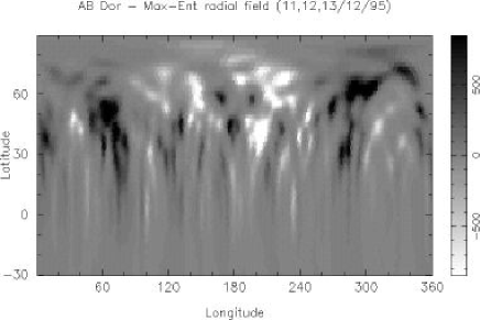
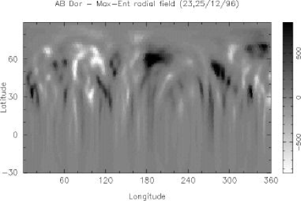
Figure 1: Zeeman-Doppler images of the surface radial field of AB Dor on 1995 Dec 11-13 (top) and 1996 Dec 23-25 (bottom). The scale bar on the right is in Gauss. Note that because the star is inclined at 60^∘ to the observer, there is limited information in the lower hemisphere.

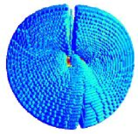
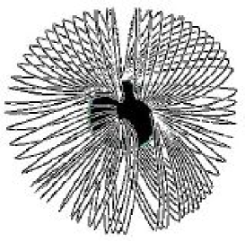
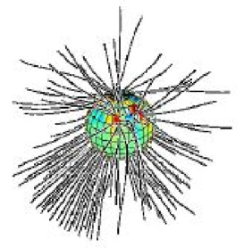
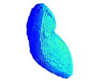
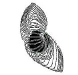
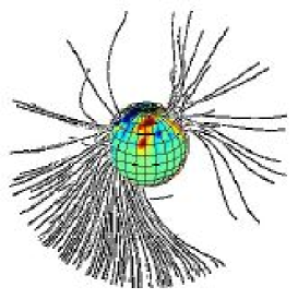
Figure 2: The global topology of the magnetic field of AB Dor for the 1995 data set. The top three panels show a view from longitude 18^∘ while the bottom panels show a view from longitude 288^∘. Panels 2 and 2 show the separator surfaces that separate the closed and open field regions. Note that the gap in the surface at the pole is due simply to problems in tracing field lines that pass directly over the pole. Panels 2 and 2 show the closed field lines just inside the separator surface and panels 2 and 2 show the open field lines just outside it. In panels 2 and 2 the surface radial map has been painted onto the stellar surface.

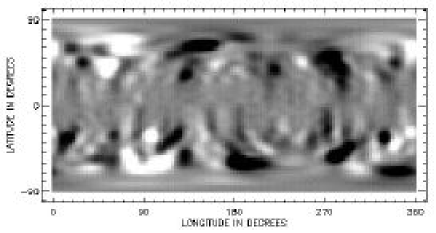
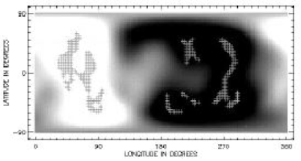
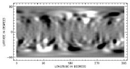
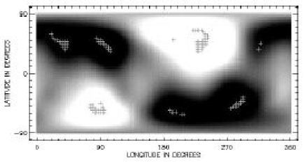
Figure 3: Images of the combined radial field with the 1995 map in the upper hemisphere and the 1996 map in the lower hemisphere. The top two panels show the case where the two maps are aligned such that both hemispheres are symmetric about the equator (positive polarity open region at the same longitude in each hemisphere). The lower two panels show an antisymmetric alignment (positive polarity open regions 180 degrees apart in longitude in the two hemispheres). Left-hand side panels show the surface radial field (greyscale extends from black at +500G to white at -500G), while panels on the right show the radial field at a height of 0.6R_⋆ above the surface (greyscale extends from black at +30G to white at -30G). The crosses mark the positions of the footpoints of the open field lines.

AB Dor is one of the most comprehensively observed of the known young rapid rotators. Long term studies of its photometric as well as its X-ray variability are available [Amado et al.2001]. It shows a small (5-13 %) rotational modulation in its X-ray emission [Kürster et al.1997] and a large emission measure of $10^{52-53}$cm^-3 [Vilhu et al.2001] consistent with a very extended or a very dense corona. The observation of large coronal prominences trapped in co-rotation with the star between 3 and 5 stellar radii from the rotation axis [Collier Cameron & Robinson1989a, Collier Cameron & Robinson1989b, Donati & Collier Cameron1997, Donati et al.1999] suggest that the corona maintains a complex structure out to large distances.

Several observations also suggest the presence of closed loops at high latitudes. Radio observations taken over a 6 month period [Lim et al.1994] have shown two prominent peaks in the emission, separated by 180^∘ of longitude. Lim et al suggest a model for directed radio emission orginating from latitudes around 60^∘. X-ray emission from such high latitudes is also believed to be responsible for the flare observed with BeppoSAX [Maggio et al.2000] which showed no rotational modulation although the observations spanned more than a whole rotation period. Since the loop height derived from modelling the flare decay phase was only 0.3R_⋆, Maggio et al claim that this flaring loop structure must have been situated above 60^∘ latitude where it would remain in view throughout a rotation cycle.

These indicators of magnetic loops at high latitude are consistent with Doppler images of AB Dor (and many other stars - see Strassmeier 1996) which show dark spots at or near the pole in addition to spots at low latitudes. Indeed, Zeeman-Doppler images (see Fig. 1) show flux at all latitudes on AB Dor (Donati & Collier Cameron 1997, Donati et al. 1999) except close to the pole where the Zeeman signal is suppressed due to the low surface brightness there. What the Zeeman-Doppler images do show at the boundary of the dark polar cap is a ring of unidirectional azimuthal field. pointer01evol suggest that this may be the result of the star’s differential rotation dragging out meridional field lines at the edge of the polar cap to form an azimuthal ring. In this case, the polarity of the field in the azimuthal ring would depend on the polarity of the field in the polar cap. In particular, the fact that this ring is of uniform polarity, would suggest that the field in the polar cap is also of one polarity. There is one significant problem with this scenario, however. If we place a unipolar field region at the pole, then some fraction of those field lines will be forced open by the pressure of the plasma they contain. If this “polar hole” extends down too far in latitude, then it will not be possible to explain the BeppoSAX observations that suggest that the closed corona extends to latitudes above 60^∘.

In this paper we use the radial magnetic field maps shown in Fig. 1 to extrapolate the coronal field. Our aim is to study the topology of the large scale field and to examine whether it is possible to reconcile the observations indicating a closed corona at high latitudes with the presence of a large polar spot.

2 Extrapolating the coronal field

We write the magnetic field ${B}$ in term of a flux function $\Psi$ such that $\mbox{\boldmath${B}$}=-\mbox{\boldmath${\nabla}$}\Psi$ and the condition that the field is potential ($\mbox{\boldmath${\nabla}$}\times\mbox{\boldmath${B}$}=0$) is satisfied automatically. The condition that the field is divergence-free then reduces to Laplace’s equation $\mbox{\boldmath${\nabla}$}^{2}\Psi=0$. A solution in terms of spherical harmonics can then be found:

$$\Psi=\sum_{l=1}^{N}\sum_{m=-l}^{l}[a_{lm}r^{l}+b_{lm}r^{-(l+1)}]P_{lm}(\theta)e^{im\phi},$$ (1)

where the associated Legendre functions are denoted by $P_{lm}$. This then gives

$$B_{r}=-\sum_{l=1}^{N}\sum_{m=-l}^{l}[la_{lm}r^{l-1}-(l+1)b_{lm}r^{-(l+2)}]P_{lm}(\theta)e^{im\phi}$$ (2)

$$B_{\theta}=-\sum_{l=1}^{N}\sum_{m=-l}^{l}[a_{lm}r^{l-1}+b_{lm}r^{-(l+2)}]\mbox{${{\displaystyle d}\over{\displaystyle d\theta}}$}P_{lm}(\theta)e^{im\phi}$$ (3)

$$B_{\phi}=-\sum_{l=1}^{N}\sum_{m=-l}^{l}[a_{lm}r^{l-1}+b_{lm}r^{-(l+2)}]\frac{P_{lm}(\theta)}{\sin\theta}ime^{im\phi}.$$ (4)

The coefficients $a_{lm}$ and $b_{lm}$ are determined by imposing the radial field at the surface and by assuming that at some height $R_{s}$ above the surface the field becomes radial and hence $B_{\theta}(R_{s})=0$ [Altschuler & Newkirk, Jr.1969]. Since large slingshot prominences are observed on AB Dor mainly around the co-rotation radius which lies at $2.7R_{\star}$ from the rotation axis, we know that much of the corona is closed out to those heights and so we set the value of $R_{s}$ to $3.4R_{\star}$. In order to calculate the field we used a code originally developed by van Ballegooijen et al. (1998).

We use three data sets, obtained on 1995 Dec 11-13, 1996 Dec 23-25 and 1998 January 10-15 (see Fig. 1). In each case we extrapolate the coronal field and distinguish between those field lines that are closed and those that are open. Fig. 2 shows some sample open field lines and also the separator surfaces that separate the regions of open and closed field. In all three cases the global topology is similar and so we show only the results for the 1995 data set. There are two dominant regions of open field lines formed at mid-latitudes about 180^∘ of longitude apart. They are of opposite polarity and hence form large helmet streamers, below which the field is predominantly closed.

3 The effect of the unobservable hemisphere

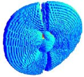
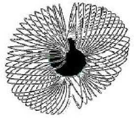
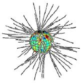
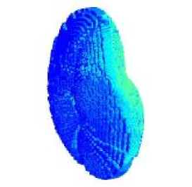
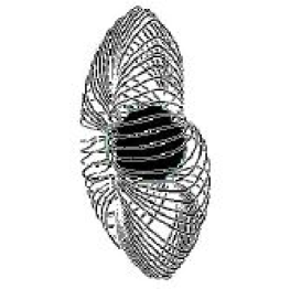
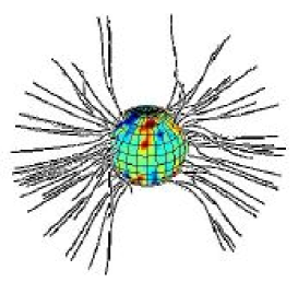
Figure 4: Global field topology for a symmetric combination of the 1995 and 1996 surface maps where positive polarity open regions are at the same longitude in each hemisphere (see also Fig. 3). The top three panels show a view from longitude 220^∘ while the bottom panels show a view from longitude 130^∘. Panels 4 and 4 show the separator surfaces that separate the closed and open field regions. Panels 4 and 4 show the closed field lines just inside the separator and panels 4 and 4 show the open field lines just outside it. In panels 4 and 4 the surface radial map has been painted onto the stellar surface.

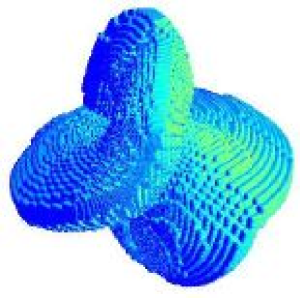
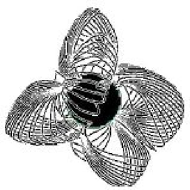
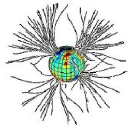
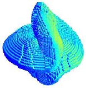
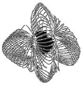
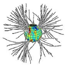
Figure 5: As Fig. 4 except that the alignment of the two maps is such that both hemispheres are anti-symmetric about the equator, with positive polarity open regions 180^∘ apart in longitude in the two hemispheres (see also Fig. 3). The top three panels show a view from longitude 308^∘ while the bottom panels show a view from longitude 128^∘.

Since the rotation axis of AB Dor is inclined at some 60^∘ to the observer, only one hemisphere can be imaged reliably. The global structure of the coronal field, however, depends on the way in which field lines originating in the observable hemisphere connect to the hidden hemisphere. Close to the surface the effect of this missing information is negligible as the small-scale fieldlines connect locally to the surface. The large-scale field is much more likely to be affected. While we have no way of determining the field structure in the hidden hemisphere, we can assess the extent of its influence. We do this by creating an artificial surface map in which the 1995 data set forms one hemisphere and the 1996 map forms the other. This produces a global field structure where the two hemispheres have similar large-scale field topologies. It is of course possible that the invisible hemisphere has a different structure to the one that we can observe. If, for example, the dynamo were to excite a mixture of modes that are symmetric and antisymmetric about the equator then the magnetic structure of the two hemispheres could be quite different. In the light of our limited information, however, we choose to make the simplest assumption, that the lowest-order field in the two hemispheres is either purely symmetric or antisymmetric about the equator. We obtain these two cases by selecting the alignment of the maps for the two hemispheres. In one case we choose a symmetric alignment, such that the two positive regions of open field in each hemisphere are at the same longitude. In the other case we place them 180^∘ of longitude apart (see Fig. 3). In the “symmetric” case, we therefore have very extended coronal holes that reach from one hemisphere into the other, while in the “anti-symmetric” case, the low-latitude field regions that were originally open now connect across the equator to form closed field regions.

In the symmetric case (Fig. 4), the closed corona is confined to a torus that covers both poles and has an axis that connects the longitudes of the open field regions. The open field regions extend across both hemispheres, reaching to fairly high latitudes, but not to the poles. In the anti-symmetric case (Fig. 5), the closed corona is a complex surface that appears to be the sum of two tori: one torus is similar to that for the symmetric case and the other torus lies in the equatorial plane and has its axis parallel to the rotation axis. This second torus is formed by field lines from low to intermediate latitudes in each hemisphere connecting across the equator.

In both cases, the structure of the high-latitude field and the longitudes of the coronal holes in the visible hemisphere are very similar. Indeed, they are very much the same as in the case where there is no field added into the hidden hemisphere at all. The main difference is in the structure of the low to intermediate latitude field. In the symmetric case, any X-ray emission would have to come from two distinct longitude bands (indeed, any prominences formed would have to originate within these bands too). This is in conflict with the wide range of rotation phases at which prominences are observed. The antisymmetric case would allow prominence formation at any longitude and also perhaps a greater X-ray emission measure, since a greater volume of the corona is closed. In the symmetric case, the volume filling factor (i.e. the volume of the closed corona as a fraction of the entire volume out to the source surface) is $0.24$, whereas in the antisymmetric case it is $0.38$.

4 The effect of flux hidden in the dark polar cap

Doppler images of AB Dor consistently show that the polar regions above latitude $\approx 70^{\circ}-80^{\circ}$ are dark. The appearance of a dark area suggests that the field in this region is strong enough to inhibit convection, but Zeeman-Doppler imaging recovers little if any field here. This is principally because the Zeeman signal is suppressed in areas of the surface that are dark. We are therefore unable to determine either the polarity or strength of this field (or indeed to determine if it is of uniform or mixed polarity).

While a dark polar cap of mixed polarity would have limited effect on the global field, the same is not true of a unipolar region. In the limiting case where this polar field dominates the field structure, the closed corona would be in the form of a torus lying in the equatorial plane and the closed field regions seen at the pole in Figs. 4 and 5 would be replaced by open field. In order to determine the extent to which such a polar field might affect the global field structure, we have added dipolar fields of different strengths to the observed surface map for 1995. The surfaces bounding the closed corona are shown in Fig. 6. A dipole field whose strength at the pole is only around 100G is sufficient to sweep the polar regions clear of closed field lines. Such a field could easily pass undetected in the Zeeman-Doppler maps, but would be insufficient to suppress convection.

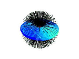
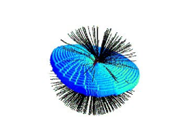
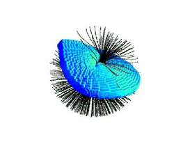
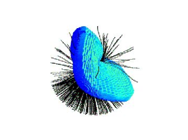
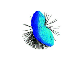
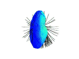
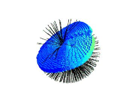
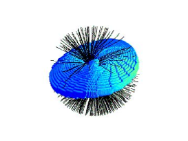
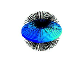
Figure 6: Surfaces separating closed and open field regions for different dipolar fields added to the surface maps. Field strengths added are: 6 1000G, 6 200G, 6 100G, 6 20G, 6 0G, 6 -20G, 6 -100G, 6 -200G, 6 -1000G. Sample open field lines are drawn in each case.

While the volume filling factor (i.e. the volume of the closed corona as a fraction of the entire volume out to the source surface) of all of these models is almost identical at $0.25$, what distinguishes them is the orientation of the torus that forms the boundary of the closed corona. In particular, there are significant differences in the latitudes at which the open field is found (and hence from which a wind could escape). The ratio of the open flux to the total flux is in fact a maximum when the imposed polar field dominates over the observed field. It should be stressed that although we have shown results for modelling the polar cap by the addition of a dipolar field to the observed field, the addition of polar spots containing the same flux as the dipole case gives qualitatively the same results.

5 The limiting case of a polar field dominating the global topology

The inevitable result of imposing a polar field that is strong enough to suppress convection is that this field dominates on the largest scales. The global field topology is just that of a dipolar field with a source surface imposed. In particular, as can be seen from 6 or 6, the polar regions are open and the polar hole extends down to a latitude that depends on our choice of the source surface position. This result appears to be in conflict with the BeppoSAX observations of maggio2000 that suggest the presence of closed loop structures at high latitudes.

In order to explore the implications of such a polar field, we can examine the tractable case of a purely dipolar field. We therefore take the $l=1,m=0$ component of (1) and impose the boundary conditions

$$B_{r}(r=R_{\star}) = 2M\cos\theta/R^{3}$$ (5)

$$B_{\theta}(r=R_{s}) = 0$$ (6)

where M is the dipole moment for a purely dipolar field and can be defined as $M=B_{r}(r=R_{\star},\theta=0)R_{\star}^{3}/2$. These boundary conditions give a “pseudo-dipole” field which can be written in terms of a correction to the classical dipole field which allows for the effect of the source surface:

$$B_{r} = \frac{2M\cos\theta}{r^{3}}\left(\frac{r^{3}+2R_{s}^{3}}{R_{\star}^{3}+2R_{s}^{3}}\right)$$ (7)

$$B_{\theta} = \frac{M\sin\theta}{r^{3}}\left(\frac{-2r^{3}+2R_{s}^{3}}{R_{\star}^{3}+2R_{s}^{3}}\right).$$ (8)

The equation of a field line is $\sin^{2}\theta=Ar/(r^{3}+2R_{s}^{3})$. The last closed field line passes through $\theta=\pi/2$ at $r=R_{s}$ and so has $A=3R_{s}^{2}$. It connects to the stellar surface at a co-latitude $\Theta_{0}$ where

$$\sin^{2}\Theta_{0}=\frac{3R_{s}^{2}R_{\star}}{R_{\star}^{3}+2R_{s}^{3}}.$$ (9)

Figure 7: Latitude of the boundary of the polar hole as a function of the source surface radius. Beyond this spherical surface the field lines are forced to be open.

Figure 8: Volume filling factor of the closed corona as a function of the source surface where the field lines are forced to be open.

Fig 7 shows how the latitude of this last closed field line varies with the imposed source surface radius $R_{s}$. For values of $R_{s}$ below about 3R_⋆ this limiting latitude decreases rapidly, and the size of the polar hole increases accordingly. The source surface would have to be placed beyond 6$R_{\star}$ to push the polar hole above 60^∘ latitude and to allow part of the closed field region to be uneclipsed, as in the Beppo-SAX flare [Maggio et al.2000]. This would reduce the fraction of open flux, since the flux of open field through the stellar surface in the upper hemisphere is just $2\pi R_{\star}^{2}\int_{0}^{\Theta_{0}}B_{r}\sin\theta d\theta$. Hence the ratio of this open flux to the total flux through the upper hemisphere is simply $\sin^{2}\Theta_{0}$. As the source surface is moved further from the stellar surface, the fraction of the flux that is open decreases.

While the amount of open flux is important to the rate at which angular momentum can be lost in a stellar wind, it is the volume of the closed corona that is relevant to the amount of X-ray emission that is produced. For this pseudo-dipole field the volume filling factor can be calculated by integrating the volume under the last closed field line whose path $\theta=h(r)$ is defined by $\sin^{2}\theta=3R_{s}^{2}r/(r^{3}+2R_{s}^{3})$:

$${\rm Volume} = 4\pi\int_{\theta=h(r)}^{\theta=\pi/2}\int_{R_{\star}}^{R_{s}}r^{2}\sin\theta drd\theta$$ (10)

$$= 4\pi\int_{R_{\star}}^{R_{s}}r^{2}\left(1-\frac{3R_{s}^{2}r}{r^{3}+2R_{s}^{3}}\right)^{1/2}dr.$$ (11)

The dependence of this volume on the position of the source surface is shown in Fig. 8. As the source surface moves closer to the star, the filling factor drops rapidly. While the X-ray emission measure also depends on the density, this shrinking of the available volume will have an increasing effect as the source surface approaches the stellar surface. Jardine & Unruh (1999) have shown that if rapid rotation strips open the outer parts of stellar coronae then this shrinking of the coronal volume with increasing rotation rate could explain the observed saturation and supersaturation of the X-ray emission .

What is clear from Fig. 7 is that in a star where the polar field dominates, the only way to have the corona extending to latitudes above about 60^∘ is to have the source surface beyond about 6$R_{\star}$. This is consistent with the observations of prominences forming between 3 and 5 $R_{\star}$, but does raise the problem of containment. The equatorial co-rotation radius on AB Dor is at some 2.7R_⋆ from the rotation axis. Beyond this point, for an isothermal corona, the density and pressure of the corona start to rise. The magnetic pressure falls with height, however, and so inevitably at some point the plasma pressure will exceed the magnetic pressure. The plasma will be able to distort and ultimately open up the field lines. Our imposition of a source surface is a crude way of modelling this process. If we place the source surface far beyond the co-rotation radius, an implausibly strong field is required to confine the plasma.

We can quantify this problem by determining the plasma pressure as a function of height for the case where the polar field dominates. If we impose hydrostatic equilibrium along a field line, then the pressure is simply

$$p=p_{0}\exp{\left(\frac{m}{kT}\oint_{s}g_{s}ds\right)}.$$ (12)

Here T is the temperature, $g_{s}$ is the component of the effective gravity along the field line, i.e. $g_{s}=({\bf g.B})/|{\bf B}|$ and

$$g(r,\theta)=\left(-GM_{\star}/r^{2}+\omega^{2}r\sin^{2}\theta,\omega^{2}r\sin\theta\cos\theta\right),$$ (13)

where $\omega$ is the angular velocity. Using (8) we can write this as

$$p(r)=p_{0}\exp{\left(-\Phi_{g}\left(1-\frac{R_{\star}}{r}\right)+\Phi_{c}\frac{(r/R_{\star})^{3}-1}{(r/R_{s})^{3}+2}C\right)}$$ (14)

where $\Phi_{g}$ and $\Phi_{c}$ are the surface ratios of the gravitational and centrifugal energies to the thermal energies, i.e.

$$\Phi_{g} = \frac{GM_{\star}/R_{\star}}{kT/m}$$

$$\Phi_{c} = \frac{\omega^{2}R_{\star}^{2}/2}{kT/m}.$$

The constant C varies from one field line to the next. If we focus on the equatorial plane, where each field line has its maximum extent $r_{m}$, then C is given by

$$C=\frac{2R_{\star}(r_{m}^{3}+2R_{s}^{3})}{r_{m}(R_{\star}^{3}+2R_{s}^{3})}.$$ (15)

The variation with height of the magnetic pressure is more straightforward. Looking just at the equatorial plane, we find that

$$|B|=\frac{2M}{r^{3}}\frac{(-r^{3}+R_{s}^{3})}{(R_{\star}^{3}+2R_{s}^{3})}.$$ (16)

Figure 9: The ratio $\beta$ of plasma to magnetic pressure along a field line as a function of radius. The field lines are forced to be open at a radius $R_{s}=6R_{\star}$.

If we now take the ratio $\beta$ of the plasma pressure to the magnetic pressure ($B^{2}/2\mu$) we find that it rises rapidly with distance above the stellar surface. If, as in Fig. 9 we put the source surface at 6$R_{\star}$, we find that the ratio $\beta$ reaches unity at around $r=3.3R_{\star}$ for a base pressure of 1Pa, a temperature of 10⁷K and a field strength at the pole of 1kG. This pressure is consistent with the results of maggio2000. The height at which $\beta=1$ is in fact fairly insensitive to our choice of parameters. Placing the source surface further out (say to 10$R_{\star}$) or dropping the coronal temperature from $10^{7}$K to $10^{6}$K moves this point out closer to 4R_⋆, but in either case, the plasma pressure is one or two orders of magnitude greater than the magnetic pressure before the source surface is reached. Even with a base pressure as low as 0.01Pa with the source surface at 10$R_{\star}$, the field lines on which $\beta>1$ do not extend above latitude 60^∘.

6 Conclusions

We have used Zeeman-Doppler images of the surface magnetic field of AB Dor to extrapolate the coronal magnetic field. This field has a clear non-axisymetric structure that becomes very apparent upon tracing the open field lines that fill much of the coronal volume. These open field lines originate in two opposite-polarity mid-latitude regions, separated by about 180^∘ of longitude. The surface separating the closed and open field regions forms a torus that passes over the visible pole. We have tried to allow for the two regions in which flux could be missing from these maps: both in the unobservable hemisphere and in the dark polar cap. Allowing for field in the unobservable hemisphere changes the field line connections at low latitudes, but the high-latitude field topology is largely unaffected. If we allow for the flux that may be concealed in the dark polar cap, we find that the polar field lines become open with the addition of a polar field so weak that it would not suppress convection sufficiently to cause the polar regions to be dark. If we impose a polar field strong enough to give a dark polar cap, we find that the large scale field is similar to that of a dipole with a source surface imposed.

This “pseudo-dipole” field does not however explain the BeppoSAX flare observations which imply high latitude closed loops. The boundary of the polar hole reaches down to latitudes well below that where observations suggest the footpoints of the flaring loop must have been located. The only way to reduce the size of the polar hole sufficiently is to move the source surface out to beyond 6$R_{\star}$. This, however, requires the pressure in the tops of the largest loops to be much greater than the magnetic pressure. The only reasonable solution seems to be to allow the polar flux to be of mixed polarity. This could be achieved by having the dark polar cap composed of many smaller spots of mixed polarity, as in the flux-emergence models of Schüssler et al. (1996), or by having a smaller polar spot surrounded by a ring of opposite polarity as in the models of Schrijver & Title (2001). Field lines in the polar spot will connect preferentially to the surrounding opposite-polarity ring, forming closed field regions at high latitudes.

If indeed young magnetically active stars do have mixed-polarity regions in their dark polar caps, there are implications for models of pre-main sequence stars. Many earlier models for the structure and formation of accretion disks and jets have rested upon the assumption that the star itself has a dipole-like field [Shu et al.1994, Lovelace, Romanova & Bisnovatyi-Kogan1995, Miller & Stone1997]. More recently, Agapitou & Papaloizou (2000) and Terquem & Papaloizou (2000) have shown that departures from a potential field or a mis-alignment of the dipole field with the stellar rotation axis (i.e. a non-axisymmetric structure) can influence the angular momentum transfer between the star and the disk or cause an observable warping of the disk. Angular momentum loss in a stellar wind is also sensitively dependent on the surface positions from which open field lines escape [Solanki, S.K., Motamen, S. & Keppens, R.1997]. In Fig. 6 the number of open field lines drawn in each panel is directly proportional to the surface area of open field lines. The nature of the field in the polar cap clearly has a significant influence on the structure of the open field and hence potentially on the spin-down rate of young stars. Our Zeeman-Doppler images imply that allowing for departures from dipolar fields is certainly justified.

References

- [\citefmtAgapitou & Papaloizou2000] Agapitou V., Papaloizou J., 2000, MNRAS, 317, 273
- [\citefmtAltschuler & Newkirk, Jr.1969] Altschuler M. D., Newkirk, Jr. G., 1969, Solar Phys., 9, 131
- [\citefmtAmado et al.2001] Amado P. J., Cutispoto G., Lanza A. F., Rodonò M., 2001, in ASP Conf. Ser. 223: 11th Cambridge Workshop on Cool Stars, Stellar Systems and the Sun. p. 895+
- [\citefmtCollier Cameron & Robinson1989a] Collier Cameron A., Robinson R. D., 1989a, MNRAS, 236, 57
- [\citefmtCollier Cameron & Robinson1989b] Collier Cameron A., Robinson R. D., 1989b, MNRAS, 238, 657
- [\citefmtDonati & Collier Cameron1997] Donati J.-F., Collier Cameron A., 1997, MNRAS, 291, 1
- [\citefmtDonati et al.1999] Donati J.-F., Collier Cameron A., Hussain G., Semel M., 1999, MNRAS, 302, 437
- [\citefmtJardine & Unruh1999] Jardine M., Unruh Y., 1999, A&A, 346, 883
- [\citefmtKürster et al.1997] Kürster M., Schmitt J., Cutispoto G., Dennerl K., 1997, A&A, 320, 831
- [\citefmtLim et al.1994] Lim J., White S., Nelson G., Benz A., 1994, ApJ, 430, 332
- [\citefmtLovelace, Romanova & Bisnovatyi-Kogan1995] Lovelace R. V. E., Romanova M. M., Bisnovatyi-Kogan G. S., 1995, MNRAS, 275, 244
- [\citefmtMaggio et al.2000] Maggio A., Pallavicini R., Reale F., Tagliaferri G., 2000, A&A, 356, 627
- [\citefmtMiller & Stone1997] Miller K. A., Stone J. M., 1997, ApJ, 489, 890+
- [\citefmtPointer et al.2002] Pointer G. R., Jardine M., Collier Cameron A., Donati J.-F., 2002, MNRAS, 330, 160+
- [\citefmtSchrijver & Title2001] Schrijver C. J., Title A. M., 2001, ApJ, 551, 1099
- [\citefmtSchüssler et al.1996] Schüssler M., Caligari P., Ferriz-Mas A., Solanki S., Stix M., 1996, A&A, 314, 503
- [\citefmtShu et al.1994] Shu F., Najita J., Ostriker E., Wilkin F., Ruden S., Lizano S., 1994, ApJ, 429, 781
- [\citefmtSolanki, S.K., Motamen, S. & Keppens, R.1997] Solanki, S.K., Motamen, S., Keppens, R., 1997, A&A, 324, 943
- [\citefmtTerquem & Papaloizou2000] Terquem C., Papaloizou J., 2000, A&A, , 1031
- [\citefmtvan Ballegooijen, Cartledge & Priest1998] van Ballegooijen A., Cartledge N., Priest E., 1998, ApJ, 501, 866
- [\citefmtVilhu et al.2001] Vilhu O., Mulhi P., Mewe R., Hakala P., 2001, A&A, 375, 492