The time delay of the quadruple quasar

Abstract

We present optical lightcurves of the gravitationally lensed components A ($\equiv$ A1+A2+A3) and B of the quadruple quasar  ($z=2.80$). The observations were primarily obtained at the Nordic Optical Telescope between 1997 March and 2001 April and consist of 74 $I$-band data points for each component. The data allow the measurement of a time delay of $146\pm 8$ days (2$\sigma$) between A and B, with B as the leading component. This value is significantly shorter than that predicted from simple models and indicates a very large external shear. Mass models including the main lens galaxy and the surrounding massive cluster of galaxies at $z=0.77$, responsible for the external shear, yield $H_{0}=71\pm 4\ ({\rm random},2\sigma)\pm 8\ ({\rm systematic})\ {\rm km\,s}^{-1}\ {\rm Mpc}^{-1}$. The systematic model uncertainty is governed by the surface-mass density (convergence) at the location of the multiple images.

1 Introduction

The light from a gravitationally lensed, multiply imaged quasar travels along slightly different paths towards the observer. This gives rise to a time delay: if the quasar is variable the same variation will be seen in the multiple images at different times. The time delay is inversely proportional to the Hubble constant, thus offering a means to measure its cosmological value in a direct way (Refsdal, 1964). Depending on the source and lens redshifts the time delay will have a weak dependence on other cosmological parameters. The time delay also depends on the gravitational potential and hence the detailed mass distribution towards the quasar, thus complicating the measurement of cosmological parameters but providing powerful constraints on distant structures such as galaxies, groups, and clusters.

With the aim of constraining cosmological parameters and the mass distribution in galaxies and clusters we have conducted a survey of time delays for multiply imaged (gravitationally lensed) quasars with the Nordic Optical Telescope (NOT). A description of the program and a measurement of the time delay in our first target, the double quasar B 1600+434 which is lensed by an edge-on disk galaxy, was presented by Burud et al. (2000). We here present the observations, data analysis and time delay of the second survey target, the quadruple quasar  ($z=2.80$) which is lensed by a galaxy and a cluster at $z=0.77$. The time delay of the third survey target, SBS 1520+530 (catalog ), is presented by Burud et al. (2002).

was discovered by Bade et al. (1997) in the ROSAT All Sky Survey. Burud et al. (1998) found optical and near infrared evidence that  is a quadruply lensed quasar with an unusual image configuration requiring a large external shear. The origin of this large external shear was attributed to a possible nearby cluster at a photometric redshift $z=0.7\pm 0.1$. Kneib, Cohen & Hjorth (2000) confirmed the existence of a massive cluster and measured the redshift $z=0.769$ and velocity dispersion $\sigma=836^{+180}_{-200}~{}{\rm km\,s}^{-1}$ of the cluster (to which the main lens galaxy belongs). From Chandra X-ray Observatory observations Morgan et al. (2001) found a cluster temperature of $2.3^{+1.8}_{-0.8}$ keV and a 2–10 keV luminosity of $7.6^{+0.6}_{-0.2}\times 10^{43}$ erg s^-1.

The three A (A1, A2, A3) components of   are very close ($\theta_{\rm A1}-\theta_{\rm A2}=0\farcs 478$, $\theta_{\rm A2}-\theta_{\rm A3}=0\farcs 608$) and the time delays between them are expected to be short, of the order of less than one week. Therefore, we focused on determining the time delay between A and B, separated by 3.1 arcsec, expected to be of the order of many months. The images are fairly bright with mean $I$-band magnitudes of 17.2 and 19.2 for A and B respectively. Early observations showed that the QSO is strongly variable with a time delay of about 200 days (Hjorth et al., 2001). We here present an analysis of the full data set.

2 Lightcurves

$I$-band images were obtained at the NOT about once a week between September 1998 and April 2001. These regular monitoring data were supplemented with a few early data points obtained at NOT and MDM between March 1997 and June 1998. The target is below the horizon at the NOT in July and August. There were additional gaps in the lightcurves due to periods of bad weather and time allocated to Spanish and international observing programs. Three different instruments were used: ALFOSC (Andalucía Faint Object Spectrograph and Camera), HiRAC (High Resolution Adaptive Camera) and the stand-by camera StanCam, equipped with detectors yielding pixel scales of 0$\farcs$189, 0$\farcs$107 and 0$\farcs$176 respectively. The $I$-band was chosen to minimize the sensitivity to lunar phase. One data point typically consisted of three exposures of 3–5 minutes each. The seeing varied from 0$\farcs$6 to 1$\farcs$5, with 0$\farcs$9 being the most frequent value. We typically obtained a signal-to-noise ratio of 200–300 for the summed A components and 50–100 for the B component.

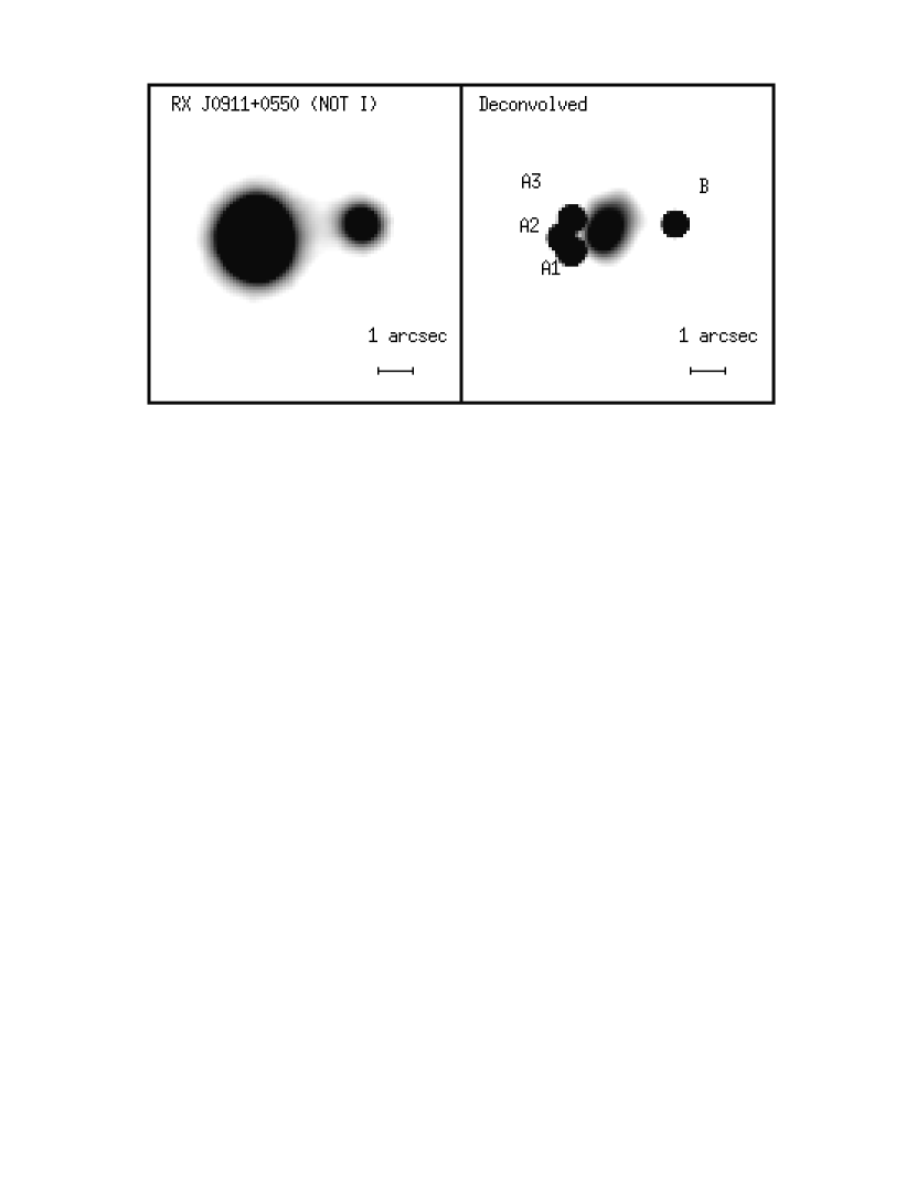
Figure 1: Stacked $I$-band images of RX J0911.4+0551 from a total of $\sim$ 7 hours of exposure. The left panel shows the combined image (seeing $=$ 1$\farcs$20). The right panel shows the deconvolved image (FWHM = 0$\farcs$28). The main lensing galaxy can be seen close to the three A components. North is up and East is to the left. Each frame measures $12\times 12$ arcsec.

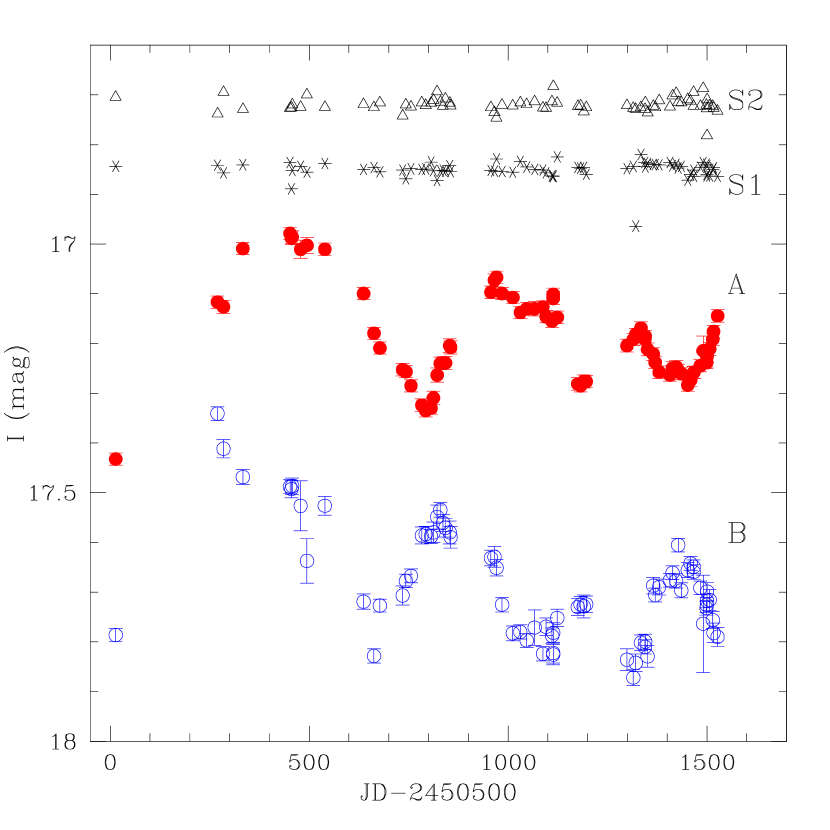
Figure 2: $I$-band lightcurves for RX J0911.4+0551 A,B and two of the stars in the field around RX J0911.4+0551 that were not used to construct the PSF. The magnitudes are calibrated using reference stars in the field (Table 1). The plotted B lightcurve is offset by $-1.5$ mag and S1 is offset by $-0.2$ mag. The error bars represent the combined photon noise and PSF errors, determined as described by Burud et al. (2000).

The data were reduced and analyzed as described by Burud et al. (2000). Preprocessing was done by dedicated pipelines while fringe correction and cosmic-ray removal were performed manually. Data from different detectors were brought onto the same photometric reference system (Burud et al., 1998) via appropriate color terms. Three reference stars with known magnitudes were used to calibrate the photometry (see Table 1 for their coordinates and magnitudes). The photometry of the quasar images was performed by applying the MCS deconvolution algorithm (Magain et al., 1998). This algorithm has already been used to analyze the data of several blended lensed quasar images (e.g., Burud et al. (1998), Burud et al. (2000)). Its main advantage is its ability to use all, even rather poor, data, irrespective of image quality and lunar phase. The final deconvolved image is produced by simultaneously deconvolving the individual frames of the same object from all epochs. The positions of the quasar images and the shape of the lensing galaxy are the same for all the frames and are therefore constrained using the total S/N of the data-set. The intensity of the point sources are allowed to vary from image to image, hence producing the lightcurves. Images of  and the resulting lightcurves are presented in Figs. 1 and 2.

3 Time delay

The $I$-band lightcurves (Fig. 2) contain 74 data points for each component. As predicted by theory, the lightcurves show that B is the leading component. A pronounced V-shaped feature at JD 2451300 (May/June 1999) is seen in the A component followed by several decreases and upturns. These are preceeded by similar features in the B component which allows the determination of a rough time delay of about 150 days. The data points are available upon request.

A quantitative analysis of the light curves was performed using the four methods described by Burud et al. (2000). The SOLA method (Pijpers, 1997) does not provide a definite time delay but is consistent with the results of the minimum dispersion method (Pelt et al., 1996) and the two novel methods introduced by Burud et al. (2001). The time-delay estimates and magnitude offsets obtained from the three different methods are consistent with each other and presented in Table 2.

It is readily apparent that no simple time translation will turn the A curve into the B curve. Thus, ‘external’ variations in the time-delay corrected flux ratios must be present. This is confirmed by our analysis of the individual A1, A2 and A3 lightcurves which exhibit similar overall trends but different detailed shapes. The time delays determined from the individual components are consistent with the expectation of small time delays between the A components and with the average B–A time delay (see Table 3).

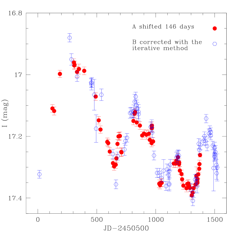
Figure 3: Combined lightcurve from both components of RX J0911.4+0551. The curve of the A component is shifted forward in time by 146 days. The B curve has been offset by values between $-1.95$ mag and $-2.05$ mag.

The ‘external’ variations, due e.g. to microlensing (see Burud et al. (2000)) are best taken into account by the methods introduced by Burud et al. (2001). In fact, the cause of the failure of the SOLA method lies in the nature of the external variations in , which are of bigher order than linear in time over the entire time series. This violates an assumption under which that method is derived. The best method for dealing with such high-order variations is the iterative method. We therefore adopt the time delay as determined by the iterative method (see Fig. 3) and conclude that the time delay between A and B in  is $146\pm 8$ days ($2\sigma$). With a $2\sigma$ error of 5 % this is among the most precise time delays determined for any lens system.

4 Discussion

In modeling the system we used a cosmology with $\Omega_{m}=0.3$, $\Omega_{\Lambda}=0.7$, and $H_{0}=100h~{}{\rm km\,s}^{-1}~{}{\rm Mpc}^{-1}$. Adopting an open Universe with $\Omega_{m}=0.3$, $\Omega_{\Lambda}=0$ increases the model time delay (and derived $H_{0}$) by 4.1 percent, whereas an Einstein–de Sitter Universe with $\Omega_{m}=1.0$, $\Omega_{\Lambda}=0$ leads to a decrease of 10.0 percent.

The ‘yardstick’ potential model of Schechter (2000) involves a two-dimensional potential given by $\psi\sim\theta^{1+\alpha}$ with $\alpha=-0.8$ and an external shear with $\kappa=\gamma=0.307$. In the adopted cosmology, this model predicts a time delay of 111$h^{-1}$ with an estimated uncertainty of $\pm 22h^{-1}$ days due to the uncertainty in $\alpha$ from the scatter in the observed shapes of nearby elliptical galaxies. In the model presented by Kneib, Cohen & Hjorth (2000) the predicted time delay is $112.5\pm 17.5h^{-1}$, consistent with the ‘yardstick’ prediction of Schechter (2000), and with a slightly smaller uncertainty.

We independently modeled the system as described by Kneib, Cohen & Hjorth (2000). The model includes the main lensing galaxy, the cluster of galaxies, and individual galaxies in the cluster. We used the measured velocity dispersion of Kneib, Cohen & Hjorth (2000) to constrain the cluster mass and adopted more realistic contraints on the ellipticity of the cluster mass distribution and a tighter mass-luminosity relation for the cluster galaxies. The main model uncertainty concerns the value of the cluster convergence $\kappa$ at the location of the multiple images. A large $\kappa$ gives rise to a small predicted time delay and derived $H_{0}$. The value of $\kappa$ is governed by the mass of the cluster, its mass profile, and the effects of possible substructure in the cluster. We find that $0.20<\kappa<0.28$ is required for a good fit. This range in $\kappa$ translates into different values for the mass and velocity dispersion of the cluster, depending on the mass profile used and the ellipticity of the cluster mass distribution. In addition to the smooth cluster convergence there is a contribution to the total convergence of about 0.06 from the individual galaxies in the cluster (not including the main lens).

The refined model prediction of the (flux-weighted or straight) mean B–A time delay is $104\pm 11h^{-1}$ (the individual time delays between the A components are less than 1.5 $h^{-1}$ days, generally in the sequence A2, A1, A3). Using the measured B–A time delay of $146\pm 8$ days (2$\sigma$), the resulting value of the Hubble constant is $H_{0}=71\pm 4\ ({\rm random},2\sigma)\pm 8\ ({\rm systematic})\ {\rm km\,s}^{-1}\ {\rm Mpc}^{-1}$.

The variability of  is sufficiently strong and erratic that the prospects for refining the time delay to better than $\pm 5$ percent are very good. Measurements of the time delays between A1, A2, and A3 also appear within reach from intensive optical or X-ray monitoring (Chartas et al., 2001). Moreover, further mapping of the cluster potential towards  from Chandra X-ray Observatory, XMM-Newton, HST, and VLT observations will help bring down the systematic model uncertainties by determining the cluster convergence at the location of the QSO images. Finally, the fairly high redshifts of the lens and source result in a sensitivity of the order of 10 percent to the adopted world model. With a smaller systematic uncertainty in the model and independent constraints on $H_{0}$ the system may be used to contrain $\Omega_{m}$ and $\Lambda$. Thus,  appears as one of the most useful individual lens systems for cosmological parameter determination and studies of the mass distribution in galaxies and clusters.

Table 1: Coordinates and $I$-band magnitudes for three reference stars in the field surrounding RX J0911.4+0551.

	RA(J2000)	Dec(J2000)	$I$
			(mag)
R1	09:11:21.16	+05:50:43.2	17.34$\pm$0.01
R2	09:11:26.54	+05:51:43.7	16.30$\pm$0.02
R3	09:11:29.08	+05:49:30.0	17.07$\pm$0.01

Table 2: Estimated time delays and $I$-band magnitude differences for RX J0911.4+0551 calculated with three different methods (Pelt et al., 1996; Burud et al., 2001).

	$\Delta$t	$\Delta m$
	(days)	(mag)
Minimum dispersion	153$\pm$3	$\cdots$
$\chi^{2}$ fit	147$\pm$4	$1.88\pm 0.01$
Iterative fit	146$\pm$4	1.95–2.05

Note. — The quoted uncertainties in the time delay estimates are $1\sigma$ errors.

Table 3: Estimated time delays for RX J0911.4+0551 calculated using the iterative method (Burud et al., 2001).

	$\Delta$t
	(days)
B–A	146$\pm$4
B–A1	143$\pm$6
B–A2	149$\pm$8
B–A3	154$\pm$16

Note. — The quoted uncertainties in the time delay estimates are $1\sigma$ errors.

References

- Bade et al. (1997) Bade, N., Siebert, J., Lopez, S., Voges, W., Reimers, D. 1997, A&A, 317, L13
- Burud et al. (1998) Burud, I., et al. 1998, ApJ, 501, L5
- Burud et al. (2000) Burud, I., et al. 2000, ApJ, 544, 117
- Burud et al. (2001) Burud, I., Magain, P., Sohy, S., Hjorth, J. 2001, A&A, 380, 805
- Burud et al. (2002) Burud, I., et al. 2002, A&A, in press
- Chartas et al. (2001) Chartas, G., Dai, X., Gallagher, S. C., Garmire, G. P., Bautz, M. W., Schechter, P. L., & Morgan, N. D. 2001, ApJ, 558, 119
- Hjorth et al. (2001) Hjorth, J., Burud, I., Jaunsen, A. O., Andersen, M. I., Korhonen, H., Clasen, J. W., & Østensen, R. 2001, in ASP Conf. Proc. 237, Gravitational Lensing: Recent Progress and Future Goals, ed. T. G. Brainerd & C. S. Kochanek (San Francisco: ASP), 125
- Kneib, Cohen & Hjorth (2000) Kneib, J.-P., Cohen, J., & Hjorth, J. 2000, ApJ, 544, L35
- Magain et al. (1998) Magain P., Courbin F., & Sohy S. 1998, ApJ, 494, 472
- Morgan et al. (2001) Morgan, N. D., Chartas, G., Malm, M., Bautz, M. W., Burud, I., Hjorth, J., Jones, S. E., & Schechter, P. L. 2001, ApJ, 555, 1
- Pelt et al. (1996) Pelt, J., Kayser, R., Refsdal, S., & Schramm, T. 1996, A&A, 305, 97
- Pijpers (1997) Pijpers, F. P. 1997, MNRAS, 289, 933
- Refsdal (1964) Refsdal S. 1964, MNRAS, 128, 295
- Schechter (2000) Schechter, P. L. 2000, in IAU Symp. 201, New Cosmological Data and the Values of the Fundamental Parameters, ed. A. N. Lasenby & A. Wilkinson, in press (astro-ph/0009048)