Spectro-photometry of galaxies in the Virgo cluster. I: The star formation history

Abstract

As a result of an extensive observational campaign targeting the Virgo cluster, we obtained integrated (drift-scan mode) optical spectra and multiwavelength (UV,U,B,V,H) photometry for 124 and 330 galaxies, respectively, spanning the whole Hubble sequence, and with $m_{p}\leq 16~{}(M_{p}\leq-15)$. These data were combined to obtain galaxy Spectral Energy Distributions (SEDs) extending from 2000 to 22000 Å. By fitting these SEDs with synthetic ones derived using Bruzual & Charlot population synthesis models we try to constrain observationally the Star Formation History (SFH) of galaxies in the rich cluster of galaxies nearest to us. Assuming a Salpeter IMF and an analytical form for the SFH, the fit free parameters are: the age ($T$) of the star formation event, its characteristic time-scale ($\tau$) and the initial metallicity ($Z$). In this work we test the (simplistic) case where all galaxies have a common age $T$=13 Gyr, exploring a SFH with ”delayed” exponential form (which we call ”a la Sandage”), thus allowing for an increasing SFR with time. This SFH is consistent with the full range of observed SEDs, provided that the characteristic time-scale $\tau$ is let free to vary between 0.1 (quasi instantaneous burst) and 25 Gyr (increasing SFR) and $Z$ between 1/50 and 2.5 Z$\odot$. Elliptical galaxies (including dEs) are best fitted with short time scales ($\tau\sim 3$ Gyr) and metallicity varying between 1/5 and 1 Z$\odot$. The model metallicity is found to increase as a function of H band luminosity. Spiral galaxies require that both $\tau$ and metallicity correlate with H band luminosity: low mass Im+BCD have sub-solar $Z$ and $\tau\geq 10$ Gyr, whereas giant spirals have solar metallicities and $\tau\sim 3$ Gyr, consistent with elliptical galaxies. Moreover we find that the SFH of spiral galaxies in the Virgo cluster depends upon the presence at their interior of fresh gas capable of sustaining the star formation. In fact the residuals of the $\tau$ vs. $L_{H}$ relation depend significantly on the HI content. HI deficient galaxies have shorter (up to a factor of 4) $\tau$ (truncated SFH) than spirals with normal HI content.

1 Introduction

One of the hottest yet unsettled issues of observational cosmology is the tracing of galaxy evolution over a large interval of look-back-time, in order to shed light on the processes that led to their formation. Currently debated formation models can be broadly divided into two categories: the hierarchical (Cole et al. 1994) or the monolithic collapse (Eggen, Lynden-Bell & Sandage 1962; Sandage 1986) models (see a review by Elmegreen 2001).
This issue can only now be pursued observationally, with the present generation of 10 m telescopes. Photometric and spectro-photometric observations of selected samples of galaxies spanning a large redshift interval can provide us with the time dependence of their structural parameters, their dynamics, their gaseous content and metal enrichment (Kauffmann & Charlot 1998) as well as their star formation histories.
An alternative approach to the issue (eg. Bell & de Jong 2000) is based on the assumption that galaxies at $z$=0 retain some memory of their past, which can be unveiled by models (e.g. Bruzual & Charlot, 1993 population synthesis models). Observations at $z$=0 would provide the boundary conditions for the modeling process.
The fundamental ingredient of both approaches is a robust observational determination of the ”end-point” of galaxy evolution: i.e. the present stage galaxy properties. Even this relatively simple point is far from settled, since the properties of local galaxies are not yet sufficiently known and understood. For example, it has been shown that the present star formation activity (per unit mass) increases along the Hubble sequence (Roberts& Haynes 1994; Kennicutt 1998), but very little attention has been given to the role of total stellar mass in determining the present evolution of galaxies, an issue that we addressed in Gavazzi et al. (1996a), Gavazzi & Scodeggio (1996), Boselli et al. (2001), and we reiterate in the present work (see also Bell & de Jong 2000 who stressed the role of the central surface brightness in regulating the evolution).
The properties of the underlying stellar population (and the physical conditions of the interstellar medium) can be best addressed using spectro-photometric measurements which are unfortunately only sparsely available. After the pioneering work of Kennicutt (1992), marginal effort was devoted at deriving the spectral parameters representative of normal galaxies in the local Universe. The work of Jansen et al. (2000), who reports on $\sim$ 200 spectra of local isolated galaxies, represents a significant exception. In the near future our knowledge of evolved galaxies will certainly benefit from the SIRTF legacy project SINGS (http://ircamera.as.arizona.edu/legacy/) by Kennicutt et al. specifically aimed at obtaining the detailed phenomenology of local galaxies through all possible observational windows.
Another aspect that lately has not been given enough consideration when studying galaxy formation and evolution is the role of environment in regulating those processes. Clusters of galaxies are ”laboratories” where galaxy evolution took place in significantly different environmental conditions from the field, the most evident signature of this being the morphology-density correlation (Dressler 1980), but other more subtle effects are known and others wait to be quantified.
With the aim of constructing a representative description of galaxies in a nearby cluster, we undertook a multi-frequency photometric survey of optically selected galaxies in the Virgo cluster, spanning the broadest possible range in morphological type (Ellipticals, spirals, dE, Im and BCD) and luminosity (-22 $\leq$ $M_{B}$ $\leq$ -15). Due to its nearness, the Virgo cluster offers a unique opportunity for carrying out such an analysis, because dwarf ($M_{B}$ $\leq$ -15) galaxies in this cluster are within reach of middle-class telescopes and, owing to the monumental photographic work of Sandage, Binggeli & Tammann which gave origin to the Virgo Cluster Catalogue (Binggeli et al. 1985; VCC), for galaxies in this cluster we can rely on a particularly accurate morphological classification.
Our own H$\alpha$, optical, near-IR, and millimetric observations, together with UV (2000 Å) and centimetric data taken from the literature, were collected in a multifrequency database.
Most recently we undertook a spectro-photometric project aimed at obtaining an homogeneous spectroscopic data-set for these galaxies. Integrated spectra of 125 Virgo galaxies have been obtained so far, covering the spectral range from 3600 to 7000 $\rm\AA$, with a resolution of $R$=500-1000. The spectra will be published in a forthcoming paper (Paper II of this series).
In the present paper we combine the newly obtained spectro-photometric data with the photometric observations to map each galaxy spectral energy distribution (SED) over a very broad wavelength range. These SEDs are then used with Bruzual & Charlot (1993, hereafter B&C) population synthesis models to constrain the star formation histories of galaxies in the Virgo cluster. The sample upon which the present work is based is discussed in Section 2. The observations are briefly described in Section 3. The construction of the galaxy SEDs, by combining photometry with spectroscopy, and their corrections are discussed in Section 4. The method adopted to fit B&C models to the data is described in Section 5. The results of this work are given in Section 6 and discussed in Section 7.

2 The sample

Table 1: The completeness in the individual photometric bands for the 598 Virgo members (or for the 312 spirals) listed in the VCC with $m_{p}\leq 16$

	N        (%)
UV	134/598  (22)
U	302/598  (51)
B	393/598  (66)
V	383/598  (64)
J	193/598  (32)
H	355/598  (59)
K	255/598  (43)
(spirals) H$\alpha$	228/312  (73)
(spirals) HI	293/312  (94)

Table 2: The available photometric measurements in the individual bands of the spectro-photometric and photometric samples, in three bins of photographic magnitude

Band	$m_{p}$	N Phot  %	N Phot+Spec  %	N $\Sigma$  %
UV	$\leq$16	57/598 (10)	63/598 (11)	120/598  (21)
”	$\leq$15	54/414 (13)	62/414 (15)	116/414  (28)
”	$\leq$14	43/248 (17)	50/248 (20)	93/248  (37)
U	$\leq$16	161/598 (27)	105/598 (18)	266/598  (45)
”	$\leq$15	150/414 (36)	94/414 (23)	244/414  (59)
”	$\leq$14	125/248 (50)	77/248 (31)	202/248  (81)
B or V	$\leq$16	206/598 (34)	124/598 (21)	330/598  (55)
”	$\leq$15	178/414 (43)	109/414 (26)	287/414  (69)
”	$\leq$14	136/248 (55)	86/248 (35)	222/248  (90)
J	$\leq$16	118/598 (20)	64/598 (11)	182/598  (31)
”	$\leq$15	105/414 (25)	57/414 (14)	162/414  (39)
”	$\leq$14	89/248 (36)	51/248 (21)	140/248  (57)
H	$\leq$16	191/598 (32)	100/598 (17)	291/598  (49)
”	$\leq$15	171/414 (41)	91/414 (22)	262/414  (63)
’	$\leq$14	134/248 (54)	77/248 (31)	211/248  (85)
K	$\leq$16	136/598 (23)	101/598 (17)	237/598  (40)
”	$\leq$15	117/414 (28)	87/414 (21)	204/414  (49)
”	$\leq$14	96/248 (39)	72/248 (29)	168/248  (68)
spir. HI	$\leq$16	114/312 (37)	86/312 (28)	200/312  (65)
”	$\leq$15	98/234 (42)	77/234 (33)	175/234  (75)
”	$\leq$14	78/150 (52)	60/150 (40)	138/150  (92)
spir. H$\alpha$	$\leq$16	92/312 (29)	87/312 (28)	179/312  (57)
”	$\leq$15	78/234 (33)	78/234 (33)	156/234  (66)
”	$\leq$14	62/150 (41)	60/150 (40)	122/150  (81)

Table 3: The completeness of the spectro-photometric and photometric samples in three bins of photographic magnitude.

mag. limit	N VCC	with z	N Phot	(%)	N Phot+Spec	(%)	N $\Sigma$	(%)
(incomplete)			220	-	125	-	345	-
$\leq$16	598	552	206	(34)	124	(21)	330	(55)
$\leq$15	414	411	178	(43)	109	(26)	287	(69)
$\leq$14	248	248	136	(55)	86	(35)	222	(90)
$\theta<2~{}or~{}4<\theta<6~{}fromM87$
(incomplete)			85	-	108	-	193	-
$\leq$16	270	244	73	(27)	108	(40)	181	(67)
$\leq$15	185	184	53	(29)	95	(51)	148	(80)
$\leq$14	107	107	28	(26)	75	(70)	103	(96)

Table 4: The new spectra in the Virgo Sample.

Obs. run	Tel.	Istr.	Resolution	Slit Width	N. Obs.
				arcsec
OHP 1998	1.93m	Carelec	500	2.5	10
OHP 1999	1.93m	Carelec	1000	2.5	17
OHP 2000	1.93m	Carelec	1000	2.5	26
OHP 2001	1.93m	Carelec	1000	2.5	24
ESO 2001	3.6m	EFOSC2	500	1.5	39
WHT 2001	4.2m	ISIS	2000	2.5	7

Table 5: The linear regression analysis

sample	regression	R	see Fig.
Ellipticals	$\rm Log\tau=-0.086\times LogL_{H}+1.351$	-0.537	11
Ellipticals	$\rm B-H=0.302\times LogL_{H}+0.599$	0.711	15
Spirals	$\rm Log\tau=-0.149\times LogL_{H}+2.221$	-0.604	13
Spirals	$\rm\Delta Log\tau=-0.132\times Def_{HI}+0.071$	-0.529	16

The Virgo Cluster Catalogue (VCC, Binggeli et al. 1985) lists 598 bona-fide Virgo cluster members brighter than $m_{p}$ = 16.0. Of these, 552 are members spectroscopically confirmed by Binggeli et al. (1993) or by Gavazzi et al. (2000c), while the remaining 46 are classified as ”possible cluster members”. Among the 598 galaxies, 312 are of late-type (from Sa to Im-BCD).
The availability of photometric data for these VCC galaxies is detailed in Table 1.
For the purpose of this paper we selected, among Virgo members with available photometry, a subsample of 330 objects (only 4 are not spectroscopically confirmed members) according to the following criteria:
1) They have the V magnitude plus at least one NIR magnitude (J or H or K; H in most cases) and at least one blue/UV magnitude (B or U or UV or H$\alpha$) measurement available. Fig.1 provides a graphical representation of this selection criterion.
2) To avoid large errors on total magnitudes that would derive from the extrapolation of poorly defined growth curves, we require B, V and NIR magnitudes to be obtained from at least 3 aperture measurements (only 5 galaxies were rejected because of this requirement. This same requirement does not apply to UV magnitudes because these are already total magnitudes).
Among these 330 objects, 124 galaxies with available spectra form the ”spectro-photometric” sample. Galaxies meeting criteria 1) and 2), but without spectroscopic observations, constitute our ”photometric sample”.
Details of the sample completeness in three bins of photographic magnitude

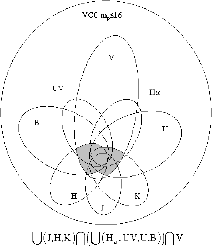
Figure 1: 330 objects meet the condition for inclusion in the ”photometric sample” (with $m_{p}\leq 16$). Of these 124, observed spectroscopically, constitute the ”spectro-photometric sample”.

Figure 2: Sky distribution of the 598 galaxies brighter than $m_{p}\leq 16.0$ in the VCC. The filled symbols represent galaxies in the spectro-photometric sample, the empty ones galaxies in the photometric sample, while the tiny symbols refer to unobserved galaxies. Elliptical galaxies are given with squares, spiral galaxies with $\rm Def_{HI}<0.5$ are triangles, spiral galaxies with $\rm Def_{HI}>0.5$ are circles. Circles are drawn at 2, 4, 6 deg. projected radial distance from M87 (cross).

and for the individual photometric bands are given separately for the ”photometric” and ”spectro-photometric” samples, and for their sum in Table 2, while the final samples and their completeness are illustrated in Table 3. Their sky distribution is shown in Fig. 2. While the global completeness of the ”spectro-photometric sample” is still rather poor at $m_{p}$ $\leq$ 16.0 (20%), it improves significantly (to 40%) over the restricted area composed by the annuli with angular distance $\theta<2$ deg and $4\leq\theta\leq 6$ from M87 where we concentrated most of our spectroscopic effort (108 spectra).
In addition to the 330 galaxies selected with the above criteria we include in our analysis 15 objects with $m_{p}$ $\geq$ 16.0 (mostly dwarf ellipticals and BCDs), out of which 14 have photometry and one (VCC636) has a spectrum available. These are: VCC 328, 636, 793, 810, 872, 882, 916, 1065, 1173, 1313, 1352, 1353, 1377, 1420, 1577. This addition brings to 345 and 125 the number of galaxies in the ”photometric” and ”spectro-photometric” samples, respectively (as listed in the first line of Table 3).
Following Gavazzi et al. (1999b) we assume a distance of 17 Mpc for the members (and possible members) of Virgo cluster A, 22 Mpc for Virgo cluster B, 32 Mpc for objects in the M and W clouds, adopting $H_{o}$ = 75 $\rm km~{}s^{-1}Mpc^{-1}$.

3 The Data

3.1 Spectro-photometry

Spectro-photometric measurements of galaxies in the Virgo cluster were taken during several runs from 1998 to 2001, using various telescopes. The detailed presentation of the spectra, including the line analysis, will be addressed in a forthcoming paper (Gavazzi et al. Paper II, in preparation). Here we give some concise information focused on the continuum spectral properties. Out of the 125 spectra used in this work, 2 were taken from the catalogue of Kennicutt (1992). Spectra of 7 BCD galaxies, obtained with the William Herschel Telescope with a resolution of 2000, were kindly provided to us by J.M. Vilchez. All the remaining spectra were obtained by us: 77 using the OHP 1.93m and 39 using the ESO 3.6m telescope (see Table 4).
The observations were taken in ”drift mode”: i.e. with the slit, generally parallel to the galaxy major axis, drifting over most of the optical surface of the galaxy (as in Kennicutt 1992). Spectra taken in this way are representative of the entire galaxy, and not only of its central regions. All spectra cover the wavelength range 3600-7000 Å  with a resolution of 500 (ESO) and 1000 (OHP). Spectra were flux-calibrated using several spectrophotometric standards. However, because of the use of drift-scan mode, their absolute flux calibration is meaningless, and therefore all spectra were normalized to their value at $\lambda=5500~{}$Å.

3.2 Photometry

Total UV, optical (U,B,V) and NIR (J,H,K) magnitudes are used to complement the spectroscopic observations in the construction of the galaxies SEDs on which this work is based.
U, B and V photometry is generally derived from our own CCD measurements. When these are not available it is derived from aperture photometry taken from the Longo et al. (1983) catalogue and the LEDA database (Prugnel & Heauderau 1998). We used only galaxies with at least three independent aperture measurements, after checking for foreground star contamination. We compute total magnitudes $\rm(U,B,V)_{25}$, i.e. magnitudes computed at the optical radius (as in Gavazzi & Boselli 1996), which are, on average, 0.1 mag fainter than the total asymptotic magnitudes.
NIR data from Nicmos3 observations, obtained by us, have been presented in Gavazzi et al. (1996b,c), Gavazzi et al. (2000a), Gavazzi et al. (2001), Boselli et al. (1997), Boselli et al. (2000). In most cases we measured the H band magnitude, in many cases the K band one, in a few cases the J band one. From these data we derive total magnitudes $\rm H_{25}$, determined as described in Gavazzi & Boselli (1996). When $\rm H_{25}$ is not available we derive it from $\rm K_{25}$ using $\rm H-K$=0.25 mag. $\rm H_{25}$ values are converted into total luminosities using: $\rm logL_{H}=11.36-0.4H_{25}+2LogD$ (in solar units), where D is the distance to the source (in Mpc). The assumed photometrical uncertainties are 15 % for B, V and H and 20 % for U, J and K (see also appendix C).
For 120 of the 345 galaxies in the photometric sample (63 in the spectro-photometric sample) UV data are available from three balloon experiments: the FOCA (Milliard et al. 1991), FAUST (Lampton et al. 1993) and SCAP (Donas et al. 1987). SCAP and FOCA use 150 Å  wide filters centered at 2000 Å, while FAUST is centered at 1650 Å ($\Delta\lambda=250\AA$). The published FOCA magnitudes (Donas et al. 1991, 1995), were recently corrected (Donas, private communication) to account for better cross-calibration between the various experiments. These are total (not aperture) UV magnitudes extracted from the photographic plates. The FAUST data were converted by us to 2000 Å  (using 0.2 mag correction on average, as concluded by Deharveng et al. 1994). The quoted error on the UV magnitude is 0.3 mag in general, but it ranges from 0.2 mag for bright galaxies to 0.5 mag for weak sources observed in frames with larger than average calibration uncertainties. We assume a conservative 0.4 mag uncertainty for all galaxies to account for all sources of systematic errors.

3.3 Other data

H$\alpha$+[NII] fluxes enter indirectly in the SEDs determination, as they provide an estimate of the ionizing flux below 912 Å  (see Section 4.1 and Appendix A). They were measured in our spectra, when available, or derived from imaging or aperture photometry by Kennicutt & Kent (1983), Almoznino & Brosch (1998), Heller et al. (1999), Koopmann et al. (2001) and references therein. Additional imaging observations of 150 galaxies have been recently obtained by us during several runs at the Observatoire d’Haute Provence (France), at Calar Alto (Spain) (Boselli & Gavazzi 2002), at San Pedro Martir (Mexico) (Gavazzi et al. 2002) and at the INT (Boselli et al. 2002). The estimated error on the H$\alpha$+[NII] flux is $\sim$ 20%.
Another important ingredient in this work, although it does not enter into the SEDs determination, is the estimate of a galaxy current neutral hydrogen content. HI data are taken from Hoffman et al. (1996, and references therein). HI fluxes are transformed into neutral hydrogen masses with an uncertainty of $\sim$ 10%. From the hydrogen mass the HI deficiency parameter ($\rm Def_{HI}$) is computed according to Giovanelli & Haynes (1985): $\rm Def_{HI}=<logM_{HI}(T^{obs},D^{obs}_{opt})>-logM^{obs}_{HI}$ where the observed HI mass is compared with the value expected from an isolated (i.e. free from external influences) galaxy having the same morphological type $\rm T^{obs}$ and optical linear diameter $\rm D^{obs}_{opt}$ (for details, see Haynes & Giovanelli 1984).

4 The galaxy SEDs

Out of the 125 obtained spectra, 119 (2 Seyfert or Liners and 4 unclassified galaxies are not included) are given in Fig. 3, grouped in 10 bins of Hubble type. These template spectra of normal cluster galaxies allow us to trace the dependence of the mean spectral properties along the Hubble sequence. Red continua characterize early type galaxies up to Sab-Sb (included), while the continua become progressively bluer for later types. Except for dEs, which have weaker absorption lines, also the line properties of galaxies up to Sab-Sb appear indistinguishable, including the 4000 Å  break. Emission lines are absent among galaxies earlier than Sa. Sa and Sab-Sb show no lines other than H$\alpha$ and [NII]. For later types the emission lines become progressively stronger, including [OIII], [OII] and the other Balmer lines. The accurate analysis of the line properties is postponed to Paper II of this series.
The method we use to constrain a galaxy star formation history consists of running B&C models with a broad grid of model parameters, and fitting the synthesized spectra to the observed ones to derive a set of best-fit parameters. However, given the limited wavelength coverage of the optical spectroscopy, a similar approach would not sufficiently narrow down the parameter space. Much stronger constraints can be derived if the spectroscopic data are combined with photometry taken over the broadest possible wavelength baseline. We thus combine our 125 spectra (“spectro-photometric sample”) with UV, optical (UBV) and infrared (JHK) photometric data. For this purpose magnitudes are converted into fluxes, then normalized at 5500 Å, as for the spectra. Before the combination, both spectroscopic and photometric data are corrected for reddening according to the prescriptions of Appendix B. In this way we obtain SEDs that cover the domain 2000–22000 Å. For 220 objects in the “photometric sample” that are not part of the “spectro-photometric” one the B&C models are fitted to the photometric data alone, as in Bell & de Jong (2000).
In order to extend our SEDs below 2000 Å  we include the estimate of the ionizing flux below

Figure 3: Template optical spectra in 10 bins of Hubble type. The number of averaged spectra in each bin is given in parenthesis. Note that the flux scale differs between the left and the right panels.

912 Å, as obtained from the H$\alpha$ flux. This is based on the assumption that the flux in the Balmer line H$\alpha$ is due to recombination of hydrogen atoms within the HII regions excited by $<912$ Å  photons from the stellar radiation field. The details of this calculation are given in Appendix A.
An example of such an extended composite SED (for the galaxy VCC 1205) is shown in Fig.4. The dots with error bars represent the available broad-band photometry with its uncertainty. The optical spectrum is represented by the thick continuous line. The dashed horizontal line in the far UV represents the $<912$ Å  flux estimate derived from H$\alpha$. The thin continuous lines represent the Bruzual & Charlot models fitted to the data (see the next section).

5 The Bruzual & Charlot models

We use the 2001 version of Bruzual & Charlot (1993) population synthesis models. These models provide the time ($T$) evolution of the synthesized spectra of galaxies characterized by an initial metallicity ($Z$), a Star Formation History (SFH) and an Initial Mass Function (IMF):

$$F_{\lambda}(T)[Z,SFH,IMF]$$ (1)

Two star formation histories are considered:
a) the exponential SFH:

$$SFR(T_{exp},\tau_{exp})=1/\tau~{}exp(-T/\tau)$$ (2)

which describes the exponential time evolution of a burst at $T$=0.
b) the ”delayed-exponential” SFH or ”a la Sandage”:

$$SFR(T_{San},\tau_{San})=T/\tau^{2}~{}exp(-T^{2}/2\tau^{2})$$ (3)

which mimics the SFH first proposed by Sandage (1986) (see Fig. 5). The temporal evolution of this family of functions is a delayed rise of the SFR up to a maximum, followed by an exponential decrease. Both the delay time and the steepness of the decay are regulated by a single parameter $\tau$.
We always assume a Salpeter IMF ($\alpha$ = 2.35 from 0.1 to 100 M$\odot$; Salpeter 1955), and explore a parameter grid in $Z$ and $\tau$. $Z$ is let free to vary from 1/50 to 2.5 Z$\odot$ in 5 steps: 0.0004, 0.004, 0.008, 0.02, 0.05. These values correspond to the initial metallicity grid computed by B&C and we have not tried to interpolate between them.

Figure 4: The extended SED of the Sc galaxy VCC 1205: the dots with error bars represent the available broad-band photometry with its uncertainty, while the observed optical spectrum is represented by the thick continuous line. The dashed horizontal line in the far UV represents the $<912$ Å  flux estimate derived from H$\alpha$. The SED is fitted with B&C models with exponential SFH and solar metallicity (thin continuous and dashed lines). In spite of having chosen two very different combinations of ages and $\tau$ ($T$=3 with $\tau$=1.8 and $T$=13 with $\tau$=20 Gyr) the two solutions have similar probabilities. This example illustrates the degeneracy between $T$ and $\tau$.

$\tau$ varies from 0.1 to 25 Gyr in 45 approximately logarithmic steps. All models are computed at two epochs: $T$=5, 13 Gyr.
Fig. 6 shows a sample of the synthetic galaxy spectra obtained assuming $T$=13 Gyr and $T_{San},\tau_{San}$, our preferred choice for these two options (see next Section). In the top panel we explore the effects of changing the time-scale of the star formation process $\tau$ while keeping the metallicity fixed at the solar value. A broad range of spectral properties is obtained, most noticeably when $\tau<5$ Gyr. In the bottom panel we keep $\tau$ fixed at 3.5 Gyr, and let $Z$ vary over its full parameter range. In this case a much narrower spectral variety is obtained.
The fitting of these synthetic spectra to the

Figure 5: The time evolution of a star formation event ”a la Sandage” is plotted for 9 values of $\tau$ from its origin ($T$=0) to 15 Gyr. This SFH is characterized by a steep rise followed by an exponential decay. It becomes progressively shallower and the position of the peak is delayed in time with increasing $\tau$. At the assumed age of 13 Gyr (vertical line) the SFH is rising for $\tau>13$ Gyr.

observed galaxy SED is carried out with a chi-squared minimization procedure that identifies the $Z$ and $\tau$ parameters for the most likely matching synthetic SED. Sometimes there is no clear minimum in the distribution of chi-squared values, and the values flatten out until one reaches the edges of the parameter grid. In this case we assign lower or upper limits (as appropriate in each single case) to the values of the corresponding parameters. Details of the fitting procedures are presented in Appendix C.

6 Results

6.1 $T$ vs. $\tau$ degeneracy

Fig. 4 shows the main limitation of our method as an age estimator: the SED of VCC 1205 is fitted with two B&C models with $T_{exp},\tau_{exp}$, solar metallicity and with very different ages ($T$=3, 13 Gyr) and decay times ($\tau$=1.8, 20 Gyr), both models giving results consistent with the observations.

Figure 6: Synthetic B&C galaxy spectra for a galaxy age $T$=13 Gyr and a star formation history “a la Sandage”. In the top panel the models have fixed initial metallicity ($Z$=0.02) and cover a range of $\tau$ values, while in the bottom panel the models have fixed $\tau=3.5$ Gyr and cover a range of $Z$ values.

Therefore, beside the well known age-metallicity degeneracy for a single stellar population (Worthey 1994), there exists another type of degeneracy that can significantly affect our attempts at deriving an accurate reconstruction of a galaxy star formation history. In fact, because of the existing strong correlation between T and $\tau$, in spite of the broad wavelength coverage of our data, our method cannot disentangle the system age from $\tau$, but it provides only $\tau$/T.
This is further illustrated in Fig.7 where the ratios $\tau_{San}/T_{San}$ computed for two different ages ($T$=5 and 13 Gyr) are plotted one against the other, showing that $\tau/T$ is approximately constant while $T$ varies by more than a factor of two. Due to this intrinsic weakness of the method we are forced to run B&C models with T fixed arbitrarily. We have chosen to use $T$=5 and 13 Gyr, but hereafter we show results only for $T$=13 Gyr, because the assumption of a common age of 5 Gyr for all galaxies appears to be at odds with the very existence of high redshift galaxies.

6.2 The choice of SFH

Having set $T$=13 Gyr we show in Fig.8 a comparison between the observed color-color ($U-V$ vs. $B-H$) relation for the galaxies in our sample and the grid of model colors obtained with the two adopted SFH (Exp, San). While both SFH reproduce without problems the reddest observed colors, the exponential SFH fails to reproduce the colors of the bluest galaxies, reaching at best a color $U-V$ $\sim$ 0.5 mag redder than observed, even assuming $\tau$=20 Gyr (quasi continuum SFH). The Sandage SFH does a better job at reproducing the full range of observed colors within the explored range of $\tau$ and metallicity, since it includes rising SFR at $T$=13 Gyr, thus allowing bluer colors. For this reason, and because it offers a more realistic time evolution of the galactic star formation history, we adopt hereafter the Sandage SFH as the best single parameterization for the star formation history of galaxies of all types. By allowing $\tau$ to assume negative values the exponential law can also have a rising SFR, but this solution is less elegant than the Sandage law. Another way to create these blue colors is through starbursts and episodic star formation, which can have considerable effect especially on small galaxies.

6.3 Fit to the template SEDs

As discussed in the previous two sections, we select the Sandage SFH as the simplest and perhaps most realistic representation of the SFH of

Figure 7: The value of the ratio $\tau_{San}$/$T_{San}$ for the best fitting model with $T$=5 Gyr against that for the best fitting model with $T$=13 Gyr, further illustrating the degeneracy between $T$ and $\tau$. Symbol shape represents Hubble type: elliptical galaxies are represented with squares, spirals with circles. Open and filled symbols differentiate galaxies in terms of HI deficiency (only for spirals): open symbols for galaxies with $\rm Def_{HI}>0.5$ while filled symbols for galaxies with $\rm Def_{HI}<0.5$. Symbol size provides an indication of the best fitting model metallicity (size is decreasing with increasing metallicity). The typical uncertainty is given in the corner of the figure.

galaxies consistent with a fixed age of $T$=13 Gyr, and we let $Z$ and $\tau$ vary as free parameters in our fitting procedure.
First we apply the fitting procedure to our templates SEDs. These were obtained extending with photometric data the spectral templates shown in Fig. 3, and are therefore very robust determinations of the typical SED for each Hubble type. The results of the fit are shown in Fig. 9. Good quality fits are obtained with $\tau$ increasing approximately monotonically along the Hubble sequence. It appears that the whole Hubble sequence can be modeled assuming increasingly delayed star formation histories of longer duration. Early type galaxies (dE, E, S0) have $\tau\leq 3$ Gyr, Sa–Sc have intermediate $4<\tau<6$ Gyr, with uncertainties $\sim 1$ Gyr. Galaxies in the 3 latest bins of Hubble

Figure 8: The observed (corrected for internal extinction) $U-V$ vs. $B-H$ color-color distribution is compared with the corresponding color-color relation obtained from the B&C models (lines) for two star formation histories: the exponential one (top) and the one “a la Sandage” (bottom) (same symbols as in Fig.7).

type are consistent with constant or even rising SFHs. Im and BCD have lower limits $\tau\geq 7$ Gyr. The behavior of the metallicity along the Hubble sequence is more erratic. Approximately solar metallicities are found mostly in early-type objects, except for dEs which show a sub-solar metallicity. Slightly sub-solar metallicities are found across the entire range of Hubble types. Beside dEs, also Im+BCD galaxies show sub-solar metallicities. Fig. 10 shows the iso-confidence contours from the fitting procedure as a function of $\tau$ and $Z$. Contours are plotted at 0.68, 0.85, 0.99 probability. The figure shows how $\tau$ is better constrained than $Z$. Typical errors on $\tau$ (see Sa, Sb, Sc) are 0.9 Gyr. The uncertainty on the metallicity is typically $\sim 0.012$, i.e. approximately one step of the metallicity grid.

6.4 The SFH of elliptical galaxies as a function of luminosity

The fit to template SEDs discussed in the previous section has shown a significant variation of the fit parameters along the Hubble sequence. In this and in the following section we apply the fitting procedure to the individual SEDs, separately for Early and Late type galaxies. The fits were inspected one by one, but due to their large number, they are not shown individually.
We explore the dependence of the fit parameters on the NIR luminosity $L_{H}$, which traces the bulk of the stellar mass. This tight correlation between stellar mass and NIR luminosity has been discussed by Gavazzi et al. (1996a) and Pierini et al. (2002) for luminous spiral galaxies, where HI mass does not dominate over the stellar mass, and by Zibetti et al. (2002) for elliptical galaxies. Thus the analysis presented in this and in the following section should shed some light on how the SFH of galaxies varies with their systemic mass.
We reiterate that individual elliptical galaxies in the ”photometric” and ”spectro-photometric” samples are fitted with B&C models with fixed SFH (Sandage) and $T$=13 Gyr and the dependence of the derived parameters $\tau$ and $Z$ are analyzed as a function of the system luminosity $L_{H}$. Fig.11 shows the shallow dependence of $\tau$ on the luminosity $L_{H}$ for elliptical galaxies (the linear regression of this and of the following relations are given in Table 5). For a range of $L_{H}$ spanning 4 decades, $\tau$ varies between 2 and 4 Gyr: i.e. these galaxies have experienced a ”short” burst of star formation in their early history (see Fig.5), with giant ellipticals being only twice ”earlier” than dEs.

Figure 9: The (corrected for internal extinction) template SEDs , obtained averaging the photometry and the individual spectra grouped in 10 bins of Hubble type (same as Fig. 3) are fitted with B&C models assuming the Sandage SFH at $T$=13 Gyr, letting $Z$ and $\tau$ as free parameters (given in the labels together with the fit probability).

Figure 10: The confidence intervals as function of $\tau$ and $Z$ for the 10 Hubble type classes (same as Fig. 9) are given with contours drawn at 0.68, 0.85, 0.99 probability.

The symbol size in Fig.11 increases with decreasing metallicity of the best fitting model. This helps showing that, beside the shallow $\tau$ vs. $L_{H}$ relation, there is a more pronounced dependence of the model initial metallicity on the system luminosity, as shown in Fig.12. At any given $L_{H}$, lower metallicity systems seem to have a lower $\tau$, due to the age-metallicity degeneracy. Summarizing, elliptical galaxies have experienced consistently ”short” bursts of star formation ”early” in their history. Their metallicity increases from sub-solar (1/5 Z$\odot$) for the dwarfs to solar for the giants.

Figure 11: The dependence of the fitted $\tau$ on H band luminosity for elliptical galaxies (same symbols as in Fig.7). Arrows mark upper and lower limits (see Appendix C).

Figure 12: The dependence of the fitted initial metallicity on H band luminosity for elliptical galaxies (same symbols as in Fig.7). A small random number has been added to the metallicity in order to avoid superposition of points.

6.5 The SFH of spiral galaxies as a function of luminosity

Figure 13 shows that the dependence of $\tau$ on the system luminosity $L_{H}$ is significantly steeper for spiral than for elliptical galaxies. Dwarf Irrs have $\tau$ of 10 or more Gyr (increasing SFR), while the most massive spirals have $\tau$ of approximately 3 Gyr, consistent with elliptical galaxies.

Figure 13: The dependence of the fitted $\tau$ on H band luminosity for spiral galaxies (same symbols as in Fig.7). Arrows mark upper and lower limits (see Appendix C).

Figure 14: The dependence of the fitted metallicity on H band luminosity for spiral galaxies (same symbols as in Fig.7). A small random number has been added to the metallicity in order to avoid superposition of points.

Once again in this figure the symbol size is inversely proportional to the metallicity of the best fitting model. While we observe a lower mean metallicity for any range of $L_{H}$ than in the case of elliptical galaxies, spirals have a global dependence of the model metallicity on $L_{H}$ not too different from the one discussed above for the ellipticals, as shown in Fig.14. This dependence of metallicity on $L_{H}$ confirms earlier findings by Bell & de Jong (2000). However, as far as $\tau$ is concerned, these authors claim that the principal correlation is the one between $\tau$ and the central K band surface brightness, followed by a less significant $\tau$ vs. $L_{K}$ relation. Our data show a marginally better correlation of $\tau$ vs. $L_{H}$ than that of $\tau$ vs. $\mu_{e}$. Notice however that we use the effective H band surface brightness $\mu_{e}$ instead of the central one used by Bell & de Jong (2000), and this might contribute to the discrepancy. We repeated the residual test of the Bell & de Jong and we find that the residuals of the $\tau$ vs. $\mu_{e}$ relation correlate with $L_{H}$ slightly better than the residuals of the $\tau$ vs. $L_{H}$ relation correlate with $\mu_{e}$. Based on our analysis alone it is therefore impossible to discriminate whether $\mu_{e}$ or $L_{H}$ is the principal parameter in regulating galaxy star formation history.

6.6 The color-magnitude relation

The color ($B-H$) vs. magnitude ($L_{H}$) relation for all galaxies, irrespective of their morphological type, is given in Fig.15. Elliptical galaxies obey to a shallow color-magnitude relation which can be understood almost exclusively in terms of increasing metallicity with mass (the metallicity of dEs is significantly lower than that of giant ellipticals), with only a marginal spread in $\tau$ in the explored luminosity range. The steeper (and non-linear) color-magnitude sequence of spirals/Im+BCD, instead, derives from the combination of increasing $Z$ and decreasing $\tau$ from dwarfs to giants. Notice that the colors of ellipticals are as red as those of spirals at the highest luminosities, suggesting a smooth transition from elliptical to spiral galaxies, with S0 galaxies in between.

Figure 15: The (corrected) color–magnitude ($B-H$ vs. $L_{H}$) relation for elliptical and spiral galaxies (same symbols as in Fig.7). The dashed line is the fit for the elliptical galaxies.

6.7 The environmental dependence of the SFH of spiral galaxies

The results of the previous sections are probably not unique to the Virgo cluster. They are consistent with Bell & de Jong (2000) analysis of non-cluster galaxies and it would not be surprising to see similar luminosity dependencies among the isolated galaxies of Jansen et al. (2000). Are there features depending on the specific cluster environment? Ideally one should investigate whether the $\tau$ - luminosity relation varies as a function of some environmental parameter, like the local galaxy density or the projected angular distance from the cluster center. However Virgo has a complex structure, reflecting its non-virialized nature, which makes this approach unfeasible. Beside the main cluster A containing M87, a number of clouds are known to exist in this cluster: cluster B dominated by M49, clouds W, M, E and S, each with different velocity or distance, or both, as analyzed by Gavazzi et al. (1999). As a result of the superposition of clouds on any line of sight, both the local galaxy density or the projected angular distance from M87 provide little indication about the real environment surrounding any given galaxy in the Virgo cluster.
We are therefore using a slightly indirect approach to the analysis of environmental effects, based on the $\rm Def_{HI}$ parameter, as defined by Giovanelli & Haynes (1985) (see also Sect. 3.3). Analyzing HI data of spiral galaxies in 9 rich clusters of galaxies, these authors concluded that HI deficiency is most likely due to ram-pressure stripping, a dynamical phenomenon occurring to galaxies in their fast motion through the cluster intergalactic medium (Gunn & Gott 1972). The extension of the sample, from the original 9 to 18 clusters, allowed Solanes at al. (2001) to conclude that the most HI deficient objects are those in radial orbits. The fact that asymmetries in the HI distribution (Dickey & Gavazzi 1991, Bravo-Alfaro et al. 2000) are often associated with radio continuum trails (Gavazzi & Jaffe 1987, Gavazzi et al. 1995) and in one case with an H$\alpha$ trail (Gavazzi et al. 2001b) pointing in the same direction as the HI asymmetry, strongly suggests that ram-pressure stripping is the most plausible explanation for the pattern of HI deficiency in clusters. Thus the $\rm Def_{HI}$ parameter can be considered an indirect indicator of the environmental conditions experimented by a galaxy over the last few Gyr. A careful inspection of Fig.13 shows that galaxies suffering from significant HI deficiency ($\rm Def_{HI}>$0.5) (empty circles) are found systematically below the regression line of the $\tau$ - luminosity relation. The residual of the $\tau$ - luminosity relation versus $\rm Def_{HI}$ is plotted in Fig.16 showing a significant trend. The deficient galaxies have SFH $\sim$4 times shorter than the unperturbed galaxies. Summarizing: spiral galaxies have luminosity dependent SFHs, and the residual of the $\tau$ - luminosity relation is found to depend on the HI content, with the gas-poor galaxies showing truncated SFH compared with cluster galaxies with normal HI content.

7 Discussion and conclusion

We have combined spectro-photometry for 125 galaxies in the Virgo cluster with broad-band photometry from UV to NIR (including an estimate of the $<912$ Å  flux from H$\alpha$). The resulting SEDs (corrected for internal extinction) were fitted with Bruzual & Charlot population synthesis models with a variety of model parameters ($SFH$, $T$, $\tau$, $Z$). The main results of the present work can be summarized as follows:

Figure 16: The residual of the relation between $\tau$ and H band luminosity for spiral galaxies (Fig.13) is given as a function of the HI deficiency parameter (same symbols as in Fig.7).

1) the observations are consistent with the simplest (minimum number of assumptions) hypothesis that the all galaxies began their formation 13 Gyr ago. This assumption implies that the star formation history of galaxies is allowed to increase with time, i.e adopting a SFH ”a la Sandage” (see Fig.5). According to this family of SFHs the SFR increases with time, reaches a maximum and decreases exponentially. A single parameter $\tau$ determines the delay of the SFR peak, thus the mean ”age” of the stellar population, as well as the shape of its time dependence: the shorter $\tau$ the more peaked the SFHs.
Having made these assumptions the Hubble sequence is obtained with increasing $\tau$ with lateness, as proposed by Sandage (1986).
2) $\tau$ is a decreasing function of the H-band luminosity. This dependence is shallow for elliptical galaxies: i.e. the value of $\tau$ for the dwarfs ($\tau\sim 4$ Gyr) and that for the giants ($\tau\sim 2$ Gyr) do not differ by more than a factor of 2, both being short compared with the assumed galaxy age (see Fig.11). Late-type galaxies display a broader range of $\tau$ values, from 25 Gyr (increasing SFR) for the low mass dwarf Im+BCD galaxies, down to 3 Gyr for the massive, early type spirals (see Fig.13).
3) the stellar metallicity increases as a function of the H-band luminosity across the entire Hubble sequence (see Figs.12 and 14). $Z$ is found to span approximately a decade from low mass to massive systems. It should however be stressed that metallicities are poorly constrained by the model.
In short: the galaxy mass, as estimated from the H-band luminosity (or perhaps the surface brightness), seems to play a crucial role in determining most galaxy structural parameters (similar dependences of several other photometric and structural parameters on H-band luminosity are discussed in Scodeggio et al. 2002).
Trying to reconcile the above results with models of galaxy formation-evolution is beyond the scope of the present investigation. We refer the reader to Elmegreen (2001) for a comparison of the predictions of the hierarchical and of the monolithic models with the observations, unfortunately not explicitly focused on the dependence of the model predictions on the galaxy mass, an issue that we would like to address in the remainder of the present discussion, at least qualitatively.
The hierarchical scenario contains an implicit reference to the mass. The mass in this model is a growing function of time (i.e. of the number of mergings). It is natural that the most massive objects (either giant ellipticals or bulge-dominated spirals), being the product of a small number of major merging events which were likely to take place at $z>2$ (Lacey & Cole 1993), can be modeled in our formalism with $\tau\sim 3$ Gyr. Low mass Im+BCD with significant current SFR, can be reconciled with the hierarchical scenario because dwarf galaxies either presently in formation or currently undergoing minor mergings are allowed by the model. Their SFH, which we model for simplicity with shallow, continuous functions, may in fact consist of a series of minor star formation bursts, associated with minor merging events (see Kauffmann, Charlot & Balogh 2001).
Our findings can in principle be reconciled also with the monolithic scenario if the mechanism of proto-galactic collapse is assumed to be not scale-free: i.e. that it depends on the total mass of the proto-galactic cloud, beside the dependence on its angular momentum. Angular momentum would discriminate between the formation of ellipticals and spirals with identical mass (Sandage 1986), whereas the system mass would further regulate the efficiency of collapse: massive proto-galaxies would undergo an early efficient collapse, while small primordial fluctuations would take a longer time to form galaxies. As discussed by Boselli et al. (2001), not only the star formation history, but also the time dependence of the gas consumption can be modeled within the monolithic scenario with the above assumption.
The additional finding of the present work is that the star formation time-scale $\tau$ of spiral galaxies in the Virgo cluster depends on their present hydrogen content. Highly HI deficient spirals in Virgo have typical time-scales ($\tau$) up to 4 times smaller than their HI healthy counterparts. If, as proposed by Giovanelli & Haynes (1985) and confirmed by Solanes et al. (2001), HI deficiency occurs to cluster spirals due to ram-pressure stripping (Gunn & Gott 1972), the exhaustion of the HI reservoir might have produced an earlier truncation of the star formation activity in these galaxies. This mechanism is invoked by Gavazzi et al. (2002) to explain the significantly quenched current star formation rate found in HI deficient Virgo spirals included in their extensive H$\alpha$ imaging survey. One might argue that the argument could be reversed: these galaxies appear HI deficient because a higher gas consumption occurred during an intense earlier star formation burst. However this reversed argument is in contradiction with the observations because it would imply that HI deficient galaxies would exist also outside clusters, something that is not observed.
Among the highly HI deficient objects with truncated SFH there are few bright Sa in our sample (VCC958 = NGC4419, VCC984 = NGC4425, VCC1047 = NGC4440, VCC1158 = NGC4461, VCC1412 = NGC4503) with $\tau$ as short as 3 Gyr. This look-back time corresponds to $z\sim 3$, suggesting that at this early cosmological epoch Virgo was a fully developed cluster with a dense IGM. This is uncomfortably close to the maximum time of cluster formation allowed by the hierarchical theory ($z\sim 2$).

Appendix A Estimate of the $<912$ Å  flux from $H\alpha+[NII]$.

The stellar radiation field with $\lambda<912$ Å  ionizes the gas which re-emits, via recombination lines. If the gas is optically thick in the Lyman continuum, the number of photons in a specific recombination line is directly proportional to the number of star photons in the Lyman continuum. In the case of H$\beta$ this number is given by equation (5.23) in Osterbrock (1989). For H$\alpha$ we have:

$$\int\limits_{\nu_{0}}^{\infty}\frac{L_{\nu}}{h\nu}d\nu=L_{H\alpha}\cdot C$$ (A1)

where:

$$1/C=h\nu_{H{\beta}}\frac{\alpha^{eff}_{H\beta}(H^{o},T)}{\alpha_{B}(H^{o},T)}\frac{F_{H\alpha}}{F_{H\beta}}$$ (A2)

Assuming $T$=10000K and the Osterbrock case B:
$\alpha^{eff}_{H\beta}(H^{o},T)=3\times 10^{-14}({\rm cm^{3}~{}sec^{-1}})$
$\alpha_{B}(H^{o},T)=2.59\times 10^{-13}({\rm cm^{3}~{}sec^{-1}})$
and $\frac{F_{H\alpha}}{F_{H\beta}}=2.87$
From the H_α luminosity it is thus possible to recover the number of ionizing photons, which can be compared with the similar quantity derived from the integral on the model spectrum.
For galaxies in the ”spectro-photometric” sample $L_{H_{\alpha}}$ is measured. For galaxies in the ”photometric” sample $L_{H_{\alpha}}$ can be in most cases derived from imaging observations. These however must first be corrected for the contamination of [NII]. From our spectra we calibrate an empirical relation between ${H\alpha}/[NII]$ and $L_{H}$ and apply it to estimate [NII] for the remaining galaxies of known $L_{H}$.
The derived $L_{H\alpha}$ must be further corrected for extinction. We assume 0.8 and 0.6 mag extinction at H$\alpha$ for galaxies earlier than Scd and for Sd-Im-BDC respectively (consistently with Boselli et al. 2001). Moreover we assume that 100% of the UV photons contribute to excite the recombination lines (Mezger 1978), with en escaping fraction of 0. A conservative estimate of the uncertainty on the derived $<912$ Å  flux is 1 mag.

Appendix B The extinction correction

The issue of determining the internal extinction in galaxies is a very controversial (from the extreme optically transparent assumption of Holmberg, 1958 to the optically thick case of Valentijn 1990) and difficult one, due to the complexity of the mutual geometry of obscuring dust and stars (Charlot & Fall 2000). Moreover stars of different ages have different scale heights, making the determination of the wavelength dependence of extinction a very uncertain task. The scale height ratio dust/stars was found to vary with $\lambda$ from 0.2 in H to 0.9 in B by Boselli & Gavazzi (1994), whereas Xilouris et al. 1999 found it approximately constant.
Solving this issue is beyond the scope of the present investigation. However we cannot avoid correcting our extended SEDs for internal extinction using some, even simplistic recipe.
The extinction corrected intensity at any $\lambda$ is related to the observed intensity by:

$$LogI_{\lambda C}=LogI_{\lambda o}+0.4\cdot A_{\lambda}$$ (B1)

where

$$A_{\lambda}=f(\tau_{\lambda})$$ (B2)

$\tau(\lambda)$ is the optical thickness at $\lambda$ and $f$ depends on the relative geometry of dust and stars.
We tested several approaches, whose results are shown in Fig. 17, carrying the SED of the moderately inclined Sc galaxy VCC 2058, before and after the correction for internal extinction.
1) We tried the Calzetti (2001, C01 hereafter) empirical absorption law derived for star-burst galaxies from the Balmer decrement (top-right panel of Fig. 17). As pointed out by Buat et al. (2002) the Calzetti law can hardly apply to normal galaxies, as it overestimates the absorption in the UV, due to the particular geometry of star-burst galaxies.
2) We derived $A_{UV}=g(FIR/UV)$ from the FIR/UV ratio, as proposed by Buat et al. (1999, 2002) and Witt & Gordon (2000; W&G00 hereafter). This choice is supported by the fact that FIR and UV fluxes are in first approximation independent from the SFH (the two are produced by similar stellar populations) and from the assumed dust-star geometry. From $A_{UV}$ we calculate $\tau_{UV}$ for 3 geometries, than we derive

$$\tau_{\lambda}=f^{\prime}(A_{\lambda})$$ (B3)

$$\tau_{\lambda}=\tau_{UV}\cdot k_{\lambda}/k_{UV}$$ (B4)

using the galactic extinction law $k(\lambda)$ (Savage & Mathis 1979), and we compute the complete set of $A_{\lambda}$ using (B2).
The assumed geometries are:
2a) the sandwich model of Disney et al. (1989, D89 hereafter) (bottom-right panel of Fig. 17). We used a $\lambda$ dependent dust to stars scale ratio: 0.86(B), 0.78(V), 0.18(H) (intermediate between the optically thick and thin case of Boselli & Gavazzi 1994).
2b) the slab model of D89 (bottom-left panel of Fig. 17).
2c) the dusty-spherical slab model (with clumpy dust distribution) of W&G00, which includes the contribution from the scattered light (top-left panel of Fig. 17).
As concluded earlier, we rule out the Calzetti law because it overestimates $A_{UV}$ in normal galaxies. Similarly we excluded the W&G00 model because the spherical approximation is hardly a realistic one. Since the sandwich and slab models of D89 produce very consistent results we finally adopted for simplicity the slab model.
In this model the explicit functional dependence of (B2) gives the face-on:

$$A_{\lambda}=2.5\cdot Log\frac{1-exp(-\tau_{\lambda}\cdot sec(i))}{\tau_{\lambda}\cdot sec(i)}$$ (B5)

where $sec(i)=a/b$. According to Buat et al. (1999) $A_{UV}$ can be quantified as:

$$A_{UV}(mag)=0.466+Log(FIR/UV)+0.433\times(Log(FIR/UV))^{2}$$ (B6)

where $FIR=1.26\times(2.58\times 10^{12}\times F_{60}+10^{12}\times F_{100})\times 10^{-26}~{}~{}~{}~{}~{}~{}[Wm^{-2}]$
$F_{60}$ and $F_{100}$ are the IRAS FIR fluxes (in Jy)
and $UV=10^{-3}\times 2000*10^{(UV_{mag}+21.175)/-2.5}~{}~{}~{}~{}~{}[Wm^{-2}]$
(B4) can be obtained from a polynomial fitting inverting (B6):

$$\tau_{UV}=(1/sec(i))\times(0.0259+1.2002\times A_{UV}+1.5543\times A_{UV}^{2}-0.7409\times A_{UV}^{3}+0.2246\times A_{UV}^{4})$$ (B7)

Thus $A_{\lambda}$ are finally obtained. FIR/UV is available for 85 objects. If FIR or UV measurements are unavailable we assume $A_{UV}$ = 1.28; 0.85; 0.68 mag for Sa-Sbc; Sc-Scd; Sd-Im-BCD galaxies respectively, as determined for galaxies in these three classes of Hubble type when FIR and UV measurements are available.
After the SEDs were corrected with the above method, we checked empirically that they do not contain a residual dependence on the galaxy inclination. The corrected SEDs of 32 Sc galaxies, binned in 4 intervals of inclination, and their fit parameters were found very consistent one another.

Appendix C Fit of B&C models to the data

The logarithmic fit of B&C models to the data is obtained minimizing the $\overline{\chi}^{2}$ (reduced chi-squared):

$$\overline{\chi}^{2}=\frac{1}{d}\sum\limits_{i=1}^{N}\left(\frac{F_{i,obs}-F_{i,mod}}{\sigma_{i}}\right)^{2}$$ (C1)

where $d$ is the number of degrees of freedom, $d=n-v$, $n$ represents the number of bands for which $F_{i,obs}\neq 0$, $v$ is the number of constraints, i.e. the number of fitted parameters (e.g. $Z$ and $\tau$). $F_{i,obs}$ and $F_{i,mod}$ are the observed and model fluxes respectively, and $\sigma_{i}$ is the error associated with each photometric ”band” (UV, U, B V, J, H, K, H$\alpha$, spectrum).

$$logF_{i,obs}=-0.4\cdot Mag_{i}+C_{i}-A(f_{i})~{}({\rm erg~{}cm^{-2}~{}sec^{-1}~{}\AA^{-1}})$$ (C2)

where
$C_{i}=-2.5\cdot\left(log(\int F_{Vega}(\lambda)R_{i}(\lambda)d\lambda\right)$
are tabulated in Table 6 and
$A(f_{i})=-2.5\cdot log(\int R_{i}(\lambda)d\lambda)$
represent the area of the filter transmission (taken from B&C).
For the B, V, H bands we assume an uncertainty of 0.15 mag, 0.2 for U, J and K, 0.4 mag for UV and a large uncertainty of 1 mag for the $<912$ Å  flux derived from H$\alpha$.
The spectra were divided in 6 bins: 3800-4000; 4000-4200; 4200-5000; 5000-5800; 5800-6600; 6600-7000 Å. The first 2 narrow bins bracket the 4000 Å  break. Each spectral bin contributes to the fit as one ”photometric point”. The error on each point was determined by combining the rms measured in line-free regions of the individual spectral bins with 0.10 mag uncertainty in the photometric calibration.
From $\overline{\chi}^{2}$ we compute a fit probability defined as:

$$P(\overline{\chi}^{2}\geq\overline{\chi}^{2}_{obs})=\frac{2}{2^{d/2}\Gamma(d/2)}\int^{\infty}_{\overline{\chi}^{2}_{obs}}x^{d-1}e^{-x^{2}/2}dx.$$ (C3)

where $\Gamma$ is the incomplete-gamma function. $P(\overline{\chi}^{2}\geq\overline{\chi}^{2}_{obs})$ is the probability of obtaining a $\overline{\chi}^{2}$ equal to the observed value ($\overline{\chi}^{2}_{obs}$). Only fits with probability $>5\%$ are considered. Only 3 galaxies in the photometric sample and none in the spectro-photometric sample have $P<5\%$, while 85 % of the objects have $P>70\%$. For any given metallicity the probability of the fit is traced as a function of $\tau$. For most cases the distribution reaches a maximum at a given $\tau$ and $Z$ which are then selected as best parameters (see Fig.18 center). In some cases the probability never reaches a maximum within the parameter space, but tends asymptotically to a maximum either for $\tau\to 0$ or $\tau\to\infty$ (see Fig.18 left and right). Because neither of these values is meaningful in these cases we adopt $\tau$, $Z$ corresponding to a threshold probability of 0.90 of the maximum.
Two notes of caution.
1) In spite of our effort for homogenizing the apertures at which data used in the present work were taken, total UV magnitudes, integrated spectra and broad band photometry have still slight aperture differences (see Section 3). The residual aperture effects on the SED shapes should however be within the quoted photometric uncertainties, thus not affecting significantly the determination of the fit parameters.
2) The incompleteness in the various observations bands increases toward lower luminosities (see Section 2). This might bias the luminosity dependence of the fit parameters. We have checked this effect by excluding one by one from the fit the UV, the U and B data and the spectra. We conclude that none of these exclusions produces significant changes. In particular excluding the U, B and spectral data does nothing but adding some noise in the correlations. The exclusion of UV data has an appreciable effect on the SEDs of some early-type spirals which become ”bluer”, thus with longer $\tau$.

Filter C UV 15.44 U 14.11 B 13.06 V 13.77 J 15.85 H 16.11 K 16.62

Table 6: Conversion coefficients from magnitude to flux for the considered filters. The coefficient for the UV filter corresponds to 2000 Å since $\rm UV_{1650}$ magnitudes are converted to 2000 Åusing an average correction of 0.2 mag (see Section 3.2).

Figure 17: The SED of VCC2058 is shown uncorrected (light curve) and corrected according to the dusty-spherical slab model of Witt & Gordon (2000) (top-left panel); Calzetti (2001) (top-right panel); the slab model of Disney et al. (1989) (bottom-left panel) and the sandwich model of Disney et al. (1989) (bottom-right panel).

Figure 18: The fit probability as a function of $\tau$ for the various metallicities. An example of P($\tau$) reaching a maximum for $\tau\to 0$ is given by VCC 758 (left). An example of P($\tau$) reaching a maximum within the parameter space is given by VCC 66 (center). In this case $\tau,Z_{max}$ are univocally determined from $P_{max}(\tau,Z$). An example of P($\tau$) reaching a maximum for $\tau\to\infty$ is given by VCC 159 (right). In the first and third case $\tau,Z_{max}$ are determined using the thresholded probability of 0.90 of their maximum.

References

- (1) Almoznino E. & Brosch N., 1998, MNRAS, 298, 931
- (2) Bell E.F., & de Jong R.S., 2000, MNRAS, 312, 497
- (3) Binggeli B., Sandage A.R., Tammann G.A., 1985, AJ, 90, 1681
- (4) Binggeli B., Popescou C.C., Tammann G.A., 1993, A&AS, 98, 275
- (5) Boselli A., Gavazzi G., 1994, A&A, 283, 12
- (6) Boselli A., Tuffs R., Gavazzi G., Hippelein H., Pierini D., 1997, A&A, 121, 507
- (7) Boselli A., Gavazzi G., Franzetti P., Pierini D., Scodeggio M., 2000, A&AS, 142, 73
- (8) Boselli A., Gavazzi G., Donas J., Scodeggio M., 2001, AJ, 121, 753
- (9) Boselli A., Gavazzi G., 2002, A&A, A&A, 386, 124
- (10) Boselli A., Iglesias-Paramo J., Vilchez J.M., Gavazzi G., 2002, A&A, A&A, 386, 134
- (11) Bravo-Alfaro H., Cayatte V., van Gorkom J.H., Balkowski C., 2000, AJ, 119, 580
- (12) Bruzual G. & Charlot S., 1993, ApJ, 405, 538 (B&C)
- (13) Buat V., Donas J., Milliard B., Xu C., 1999, A&A, 352, 371
- (14) Buat V., & Xu C., 1996, A&A, 306, 61
- (15) Calzetti D., 2001, PASP, 113, 1449 (C01)
- (16) Charlot S., & Fall S., 2000, ApJ, 539, 718
- (17) Cole S., Aragon-Salamanca A., Frenk C.S., Navarro J.F., Zepf S.E., 1994, MNRAS, 271, 781
- (18) Deharveng J., Sasseen T., Buat V., Bowyer S., Lampton M., Wu X., 1994, A&A, 289, 715
- (19) Dickey J. & Gavazzi G., 1991, ApJ, 373, 347
- (20) Disney M.J., Davies J.I., Phillipps S., 1989, MNRAS, 239, 939 (D89)
- (21) Donas J., Deharveng J., Laget M., Milliard B., Huguenin D., 1987, A&A, 180, 12
- (22) Donas J., Milliard B., Laget M., Buat V., 1990, A&A, 235, 60
- (23) Donas J., Milliard B., Laget M., 1995, A&A, 303, 661
- (24) Dressler A., 1980, ApJ, 236, 351
- (25) Eggen O.J., Lynden-Bell D., Sandage A.R., 1962, ApJ, 136, 748
- (26) Elmegreen B.G., 2001, Astro-ph 0110149
- (27) Gavazzi G. & Jaffe W., 1987, A&A, 186, L1
- (28) Gavazzi G., Boselli A., 1996, Astro. Lett. and Communications, 35, 1
- (29) Gavazzi G., Pierini D., Boselli A., 1996a, A&A, 312, 397
- (30) Gavazzi G., Pierini D., Baffa C., Lisi F., Hunt L., Randone I., Boselli A., 1996b, A&A, 120, 521
- (31) Gavazzi G., Pierini D., Boselli A., Tuffs R., 1996c, A&A, 120, 489
- (32) Gavazzi G., Scodeggio M., 1996, 312, L29
- (33) Gavazzi G., Boselli A., Scodeggio M., Pierini D., Belsole E., 1999b, MNRAS, 304, 595
- (34) Gavazzi G., Franzetti P., Scodeggio M., Boselli A., Pierini D., Baffa, C., Lisi, F., Hunt, L., 2000a, A&AS, 142, 65
- (35) Gavazzi G., Franzetti P., Scodeggio M., Boselli A., Pierini D. 2000b, A&A, 361, 863
- (36) Gavazzi G., Bonfanti, C., Pedotti P., Boselli A., Carrasco L., 2000c, A&AS, 146, 259
- (37) Gavazzi G., Zibetti S., Boselli A., Franzetti P., Scodeggio M., Martocchi S., 2001, A&A, 372, 29
- (38) Gavazzi G., Mayer L., Boselli A., Vilchez P., Iglesias-Paramo J., Carrasco L., 2001b, ApJ, 563. L23
- (39) Gavazzi G., Boselli A., P. Pedotti, Gallazzi, A., L. Carrasco, 2002, A&A, A&A, 386, 114
- (40) Giovanelli R. & Haynes M.P., 1985, ApJ, 292, 404
- (41) Gunn J.E. & Gott J.R.III, 1972, ApJ, 176, 1
- (42) Haynes M.P. & Giovanelli R., 1984, AJ, 89, 758
- (43) Heller A., Almoznino E., Brosch N., 1999, MNRAS, 304, 8
- (44) Hoffman G.L., Salpeter E.E., Farhat B., Roos T., Williams H., Helou G., 1996, ApJS, 105, 269
- (45) Holmberg E., 1958, Medn. Lunds. Astr. Obs. 2, 136
- (46) Jansen R.A., Fabricant D., Franx M., Caldwell N., 2000, ApJS, 126, 331
- (47) Kauffmann G. & Charlot S., 1998, MNRAS, 294, 705
- (48) Kauffmann G., Charlot S., Balogh M., 2001, Astro-ph:0103130
- (49) Kennicutt R.C.Jr., 1992, ApJ, 388, 310
- (50) Kennicutt R.C.Jr., 1998, ARA&A, 36, 189
- (51) Kennicutt R.C.Jr. & Kent S.M., 1983, AJ, 88, 1094
- (52) Koopmann R.A., Kenney J.D.P., Young J., 2001, ApJ, 135, 125
- (53) Lacey C. & Cole S., 1993, MNRAS, 262, 627
- (54) Lampton M., Sasseen T., Wu X., Bowyer S., 1993, Geophys. Res. Lett., 20, 539
- (55) Longo G., de Vaucouleurs, A., Corwin H.G.Jr., 1983, General catalogue of photoelectric magnitudes and colors in the U,B,V system of 3,578 galaxies brighter than the 16-th V-magnitude (1936-1982) The University of Texas Monographs in Astronomy, Austin
- (56) Mezger P.O., 1978, A&A, 70, 565
- (57) Milliard B., Donas J., Laget M., 1991, Advances in Space Research, Vol. 11, 135
- (58) Osterbrock D.E., ”Astrophysics of Gaseous Nebulae and Active Galactic Nuclei”, 1989, University Science Books, Mill Valley.
- (59) Pierini D., Gavazzi G., Franzetti P., Scodeggio M., Boselli A., 2002, MNRAS, 332, 422
- (60) Prugnel P. & Heauderau P., 1998, AAS, 128, 299
- (61) Roberts M.S. & Haynes M.P., 1994, ARA&A, 32, 115
- (62) Salpeter E.E., 1955, ApJ, 121, 161
- (63) Sandage A.R., 1986, A&A, 161, 89
- (64) Savage B.D. & Mathis J.S., 1979, ARA&A, 17, 73
- (65) Scodeggio M., Gavazzi G., Boselli A., Franzetti P., Zibetti S., Pierini D., 2002, A&A, 384, 812
- (66) Solanes J.M., Manrique A., Garcia-Gomez C., Gonzales-Casado G., Giovanelli R. & Haynes M.P., 2001, ApJ, 548, 97
- (67) Valentijn E. A., 1990, Nature, 346, 153
- (68) Xilouris E. M., Byun Y. I., Kylafis N. D., Paleologou E. V., Papamastorakis J., 1999, A&A, 344, 868
- (69) Witt A.N. & Gordon K.D., 2000, ApJ, 528, 799 (W&G00)
- (70) Worthey G., 1994, ApJS, 95, 107
- (71) Zibetti S., Gavazzi G., Scodeggio M., Franzetti P. & Boselli A., 2002, A&A, submitted