The Kurtosis of the Cosmic Shear Field

Abstract

We study the fourth-order moment of the cosmic shear field using the dark matter halo approach to describe the nonlinear gravitational evolution of structure in the universe. Since the third-order moment of the shear field vanishes because of symmetry, non-Gaussian signatures in its one-point statistics emerge at the fourth-order level. We argue that the shear kurtosis parameter $S_{\gamma,4}\equiv\langle{\gamma_{i}^{4}}\rangle_{c}/\langle{\gamma_{i}^{2}}\rangle^{3}$ may be more directly applicable to realistic data than the well-studied higher-order statistics of the convergence field, since obtaining the convergence requires a non-local reconstruction from the measured shear field.

We compare our halo model predictions for the variance, skewness and kurtosis of lensing fields with ray-tracing simulations of cold dark matter models and find good agreement. The shear kurtosis calculation is made tractable by developing approximations for fast and accurate evaluations of the 8-dimensional integrals necessary to obtain the shear kurtosis. We show that on small angular scales, $\theta\lower 2.15277pt\hbox{$\;\buildrel<\over{\sim}\;$}5^{\prime}$, more than half of the shear kurtosis arises from correlations within massive dark matter halos with $M\lower 2.15277pt\hbox{$\;\buildrel>\over{\sim}\;$}10^{14}M_{\odot}$. The shear kurtosis is sensitive to the matter density parameter of the universe, $\Omega_{\rm m0}$, and has relatively weak dependences on other parameters. Therefore, a detection of the shear kurtosis can be used to break degeneracies in determining $\Omega_{\rm m0}$ and the power spectrum amplitude $\sigma_{8}$ so far provided from measurements of the two-point shear statistics. The approximations we develop for the third- and fourth-order moments allow for accurate halo model predictions for the 3-dimensional mass distribution as well. We demonstrate their accuracy in the small scale regime, below 2 Mpc, where analytical approaches used in the literature so far cease to be accurate.

1 Introduction

Weak gravitational lensing caused by the large-scale structure of the universe has been established as a useful probe of cosmological parameters and offers the possibility of directly measuring the dark matter power spectrum (see Mellier 1999 and Bartelmann & Schneider 2001 for reviews). Several independent groups have reported significant detections of lensing by large-scale structure on distant galaxy images (cosmic shear) from the ground [Van Waerbeke et al. 2000, Wittman et al. 2000, Bacon, Refregier & Ellis 2000, Kaiser, Wilson & Luppino 2000, Maoli et al. 2001, Van Waerbeke et al. 2001a, Hoekstra et al. 2002, Bacon et al. 2002] and from space [Rhodes, Refregier & Groth 2001, Haemmerle et al. 2002, Refregier, Rhodes & Groth 2002]. These groups measured the two-point correlation function of the cosmic shear field or the variance of the filtered shear field and set constrains on cosmological parameters, in particular some combination of the overall amplitude of matter power spectrum ($\sigma_{8}$) and the matter density parameter of the universe ($\Omega_{\rm m0}$), as shown in earlier theoretical work [Blandford et al. 1991, Miralda-Escude 1991, Kaiser 1992, Villumsen 1996, Bernardeau, Van Waerbeke & Mellier 1997, Jain & Seljak 1997, Kaiser 1998].

It has been shown that the non-Gaussian signature in the weak lensing field induced by nonlinear gravitational clustering can be used to break degeneracies in the determination of $\sigma_{8}$ and $\Omega_{\rm m0}$ (Bernardeau, Van Waerbeke & Mellier 1997; Jain & Seljak 1997). This possibility is attractive, since it can determine $\Omega_{\rm m0}$ via weak lensing measurements without invoking any other methods such as the cosmic microwave background (CMB) and galaxy redshift surveys. This also indicates that the dark energy component of the universe can be constrained by combining lensing measurements with the evidence for a flat universe revealed by the measured CMB angular power spectrum (e.g., Netterfield et al. 2001). Most theoretical work so far has focused on the non-Gaussian signatures described by the higher-order moments of the filtered convergence field (Bernardeau et al. 1997; Jain & Seljak 1997; Hui 1999; Van Waerbeke, Bernardeau & Mellier 1997; Jain, Seljak & White 2000; Van Waerbeke et al. 2001b; Munshi & Jain 2001) or the skewness parameter in the aperture mass map [Schneider et al. 1998, Bartelmann & Schneider 2001]. It was recently also proposed that the genus curve or Minkowski functionals of the convergence field could be an efficient measure of the non-Gaussian signal [Sato et al. 2001, Matsubara & Jain 2001, Taruya et al. 2002]. Unfortunately these methods turn out to have limitations in application to realistic data. Because realistic data has a non-trivial survey geometry with many masked areas due to light scattering, bright stars and so on, it is very challenging to reconstruct the convergence from the measured shear field. On the other hand, although the aperture mass method has the advantage of being directly obtained from the shear map, it is likely to suffer from low signal-to-noise ratio for the skewness measurement, because this method uses a compensated filter [Schneider 1996, Schneider et al. 1998] and thus leads to the loss of the non-Gaussian signal, especially on angular scales smaller than a few arcminutes where the signal is large (see Van Waerbeke et al. 2001a for detailed comparisons between various two-point statistical measures of the shear field for actual data).

Very recently, Bernardeau, Van Waerbeke & Mellier (2002a; hereafter BvWM) proposed that some specific patterns in the three-point function of the shear field can be used to extract the non-Gaussian signal. Bernardeau, Mellier & Van Waerbeke (2002b) then reported a detection of this signal from actual data on $2-4$ arcminutes scales, although the signal-to-noise so far is not enough to put robust constraints on $\Omega_{\rm m0}$. The method proposed by BvWM appears to be a promising new measure of non-Gaussianity. It is possible that their method loses some non-Gaussian information because the vector-like property of their statistic leads to partial cancellations between the signal on averaging. Their method also seems to have the limitation that it cannot extract the signal on small scales ($\theta_{\rm s}\lower 2.15277pt\hbox{$\;\buildrel<\over{\sim}\;$}2^{\prime}$), since their three-point function decreases for smaller scales and approaches zero at zero separation.

The purpose of this paper is to develop an alternative statistical method directly applicable to the cosmic shear data. The method we propose is the connected part of the fourth-order moment of the filtered shear field, in particular the shear kurtosis parameter defined by $S_{\gamma,4}=\langle{\gamma_{i}^{4}}\rangle_{c}/\langle{\gamma_{i}^{2}}\rangle^{3}$, since the non-Gaussian signal appears first at the fourth-order level for the one-point statistics. The kurtosis parameter collapses the information in the trispectrum into a single less noisy quantity, although it does not retain the full information in the four-point statistics.

Since the shear field on relevant angular scales is affected by the nonlinear regime of structure formation (e.g., see Jain & Seljak 1997), we need a model to correctly describe the redshift evolution and statistical properties of gravitational clustering up to the four-point level. The perturbation theory well studied in the literature may not be adequate for this task. On the one hand, it is known that the so-called ‘hyper-extended perturbation theory’ [Scoccimarro & Friemann 1999] can describe the strongly nonlinear clustering regime (see for Hui 1999, van Waerbeke et al. 2001b and Munshi & Jain 2001 for application to weak lensing). However, the model does not describe the intermediate-scale transition between the linear and strongly nonlinear regimes [Cooray & Hu 2001a, Scoccimarro et al. 2001], which does affect weak lensing statistics on a range of scales because of projection effects. We therefore choose to employ the dark matter halo approach, where gravitational clustering is described in terms of correlations between and within dark matter halos (see McClelland & Silk 1977; Peebles 1980; Scherrer & Bertschinger 1991 for initial applications; for recent developments see e.g. Sheth & Jain 1997; Komatsu & Kitayama 1999; Seljak 2000; Ma & Fry 2000; Scoccimarro et al. 2001; Cooray, Hu & Miralda-Escude 2000; Cooray & Hu 2001a,b; and Cooray & Sheth 2002 for a recent review). There are several reasons we use the halo model. First, the halo model is formally complete and simple enough that higher-order statistics of the weak lensing fields can be analytically calculated. Second, the results can be interpreted in terms of halo properties, which is convenient for comparison with other observations such as $X$-ray and optical surveys of clusters of galaxies. Finally, the model appears remarkably successful in that, even though it relies on rather simplified assumptions, it has reproduced results from numerical simulations [Seljak 2000, Ma & Fry 2000, Scoccimarro et al. 2001] and also allowed for interpretations of observational results of galaxy clustering [Seljak 2000, Scoccimarro et al. 2001, Guzik & Seljak 2002, Seljak 2002].

Once the three ingredients of the halo model (halo profile, mass function and halo bias) are specified, it is straightforward to develop the formalism to calculate the shear kurtosis. Cooray & Hu (2001a) have investigated the bispectrum of the convergence field using the halo model and find the convergence skewness is mainly due to rare and massive halos on relevant scales of $\theta_{\rm s}\lower 2.15277pt\hbox{$\;\buildrel<\over{\sim}\;$}10^{\prime}$, which is referred to as the 1-halo term in this paper. We will also find that the shear kurtosis arises mainly from the 1-halo term on the relevant scales. However, since the direct application of the halo model requires an 8-dimensional integration to obtain the 1-halo term, we develop an approximation that significantly reduces the computational time and gives the shear kurtosis with $10\%$ accuracy at most on angular scales of interest. Our model predictions will be compared in detail with ray-tracing simulation results for all the statistical measures we investigate: the convergence or shear variance, the convergence skewness and the kurtosis parameters of the convergence and shear fields. This comparison addresses the broader issue of whether the halo model can accurately describe statistical properties of weak lensing fields for higher-order moments beyond the two-point statistics well studied in the literature. We will pay special attention to the dependences of the shear kurtosis on the cosmological parameters, $\Omega_{\rm m0}$ and $\sigma_{8}$, for flat CDM (cold dark matter) models.

The outline of this paper is as follows. In §2 we present the dark matter halo model used in this paper and then write down the expressions for the power spectrum, bispectrum and trispectrum for the underlying density field. In §3 we investigate the validity of the halo model for weak lensing statistics by comparing the predictions with the ray-tracing simulation results for the variance and skewness of the filtered convergence field. In §4 we develop an approximation for calculating the convergence kurtosis and extend it to the shear kurtosis calculation in §5. The dependence of the shear kurtosis on cosmological parameters is presented in §6. Finally, §7 is devoted to a summary and discussion. In the following, without explicit mention we will often consider two CDM models: one is the SCDM model with $\Omega_{\rm m0}=1$, $h=0.5$ and $\sigma_{8}=0.6$ and the other is the $\Lambda$CDM model with $\Omega_{\rm m0}=0.3$, $\Omega_{\lambda 0}=0.7$, $h=0.5$ and $\sigma_{8}=0.9$, respectively. Here, $\Omega_{\rm m0}$ and $\Omega_{\lambda 0}$ are the present-day density parameters of matter and cosmological constant, $h$ is the Hubble parameter, and $\sigma_{8}$ is the rms mass fluctuations of a sphere of $8h^{-1}$Mpc radius. The choice of $\sigma_{8}$ for each model is motivated by the cluster abundance analysis [Eke, Cole & Frenk 1996].

2 Dark matter halo approach

2.1 Ingredients

In the dark matter halo approach the underlying density field can be described in terms of correlations between and within dark matter halos, which are taken to be locally biased tracers of density perturbations in the linear regime. The method is therefore based on three essential ingredients well studied in the literature: the mass function of dark matter halos, the halo biasing function, and the halo density profile.

For the halo mass function, we adopt an analytical fitting model proposed by Sheth & Tormen (1999), which is more accurate on cluster mass scales than the original Press-Schechter model [Press & Schechter 1974]. The number density of halos with mass in the range between $M$ and $M+dM$ is given by

$$\frac{dn}{dM}dM = \frac{\bar{\rho}_{0}}{M}f(\nu)d\nu$$ (1)

$$= \frac{\bar{\rho}_{0}}{M}A[1+(a\nu)^{-p}]\sqrt{a\nu}\exp\left(-\frac{a\nu}{2}\right)\frac{d\nu}{\nu},$$

where $\nu$ is the peak height defined by

$$\nu=\left[\frac{\delta_{c}(z)}{D(z)\sigma(M)}\right]^{2},$$ (2)

$\bar{\rho}_{0}$ is the mean cosmic mass density today (we use comoving coordinates throughout) and the numerical coefficients $a$ and $p$ are empirically fitted from N-body simulations as $a=0.707$ and $p=0.3$. The coefficient $A$ is set by the normalization condition $\int_{0}^{\infty}\!d\nu f(\nu)=1$, leading to $A\approx 0.129$. Here $\sigma(M)$ is the present-day rms fluctuations in the matter density top-hat smoothed over a scale $R_{M}\equiv(3M/4\pi\bar{\rho}_{0})^{1/3}$, $D(z)$ is the growing factor (e.g., see Peebles 1980), and $\delta_{c}(z)$ is the threshold overdensity for spherical collapse model (see Nakamura & Suto 1997 and Henry 2000 for useful fitting functions). It should be noted that the peak height $\nu$ is given as a function of $M$ at any redshift.

Mo & White (1996) developed a useful formula to describe the bias relation between the dark matter halo distribution and the underlying density field. This idea has been improved by several authors using N-body numerical simulations [Mo, Jing & White 1997, Sheth & Lemson 1999, Sheth & Tormen 1999]; we will use the fitting formula of Sheth & Tormen (1999) for consistency with the mass function (1):

$$b(\nu)=1+\frac{a\nu-1}{\delta_{c}}+\frac{2p}{\delta_{c}(1+(a\nu)^{p})},$$ (3)

where we have assumed scale-independent bias and neglected the higher order bias functions $(b_{2},b_{3},\cdots)$ that have a negligible effect on our final results.

The density profile of dark matter halos is defined to be an average over all halos with a given mass $M$ and does not necessarily assume all halos have the same profile and spherical symmetry as stressed by Seljak (2000). It is not evident that this argument should be valid for the higher-order moments of the density field or the weak lensing field. However, the agreement between our model predictions and numerical simulations indicates that there is no strong violation of the assumption. Throughout this paper we assume the NFW model for the averaged halo profile (Navarro, Frenk & White 1996, 1997; hereafter NFW):

$$\rho(r)=\frac{fc^{3}M}{4\pi r_{\rm vir}^{3}}\frac{1}{cr/r_{\rm vir}(1+cr/r_{\rm vir})^{2}},$$ (4)

where $f=1/[\ln(1+c)-c/(1+c)]$ and $r_{\rm vir}$ is the virial radius of the halo. The virial radius can be expressed in terms of the halo mass $M$ and redshift $z$ based on the spherical collapse model: $M=(4\pi r_{\rm vir}^{3}/3)\bar{\rho}_{0}\Delta(z)$, where $\Delta(z)$ is the overdensity of collapse given as a function of redshift (e.g., see Nakamura & Suto 1997 and Henry 2000 for a useful fitting formula). We have $\Delta\approx 340$ for the $\Lambda$CDM model. It is worth noting that some studies based on N-body simulations with higher resolution than in NFW have suggested a steeper slope for the inner profile with $\rho\propto r^{-1.5}$ at $r\lower 2.15277pt\hbox{$\;\buildrel<\over{\sim}\;$}r_{\rm vir}/c$ [Fukushige & Makino 1997, Moore et al. 1998, Jing & Suto 2000, Fukushige & Makino 2001], whereas the predictions for the outer parts of halos are in agreement with NFW: $\rho\propto r^{-3}$ at $r\lower 2.15277pt\hbox{$\;\buildrel>\over{\sim}\;$}r_{\rm vir}/c$. Lensing statistics on angular scales of interest are affected more strongly by the outer part of the density profile. Further the outer profile is scaled by the concentration parameter $c$ for a given virial radius, so we simply assume the NFW profile and pay close attention to the appropriate choice of $c$ as discussed below.

To give the halo profile in terms of $M$ and $z$, we further need to express the concentration parameter $c$ in terms of $M$ and $z$; however, this still remains somewhat uncertain. The concentration $c$ is theoretically expected to be a weak function of halo mass as given by $c=c_{0}(M/M_{\ast})^{\beta}$, where the normalization is $c_{0}\sim O(10)$ at the present-day nonlinear mass scale $M_{\ast}$ defined by $\delta_{c}(z=0)/\sigma(M_{\ast})=1$ and the slope is $\beta\sim-O(10^{-1})$. We employ the form motivated by Seljak (2000):

$$c(M,z)=10(1+z)^{-1}\left(\frac{M}{M_{\ast}(z=0)}\right)^{-0.2},$$ (5)

where we have assumed the redshift dependence $(1+z)^{-1}$ as supported by numerical simulations [Bullock et al. 2001]. There are several reasons we adopt the form (5) for the unknown concentration parameter. As for the slope $\beta$, we assume $\beta=-0.2$ which is steeper than $\beta=-0.13$ originally proposed by NFW and Bullock et al. (2001). This is motivated by the fact that for the NFW profile (4) the halo model with $\beta=-0.2$ can better reproduce the well-studied nonlinear matter power spectrum than the model with $\beta=-0.13$ as shown in Seljak (2000; also see Cooray et al. 2000). As will be shown below, our model can also reproduce the simulation results for the higher-order statistics of weak lensing fields on relevant angular scales. In this sense, for the purpose of using the halo model to describe the nonlinear gravitational evolution, it seems to be appropriate to choose the halo model parameters so that the model can reproduce the matter power spectrum as the first step. The choice of the normalization of $c_{0}=10$ at $M_{\ast}$ is supported by N-body simulations (Bullock et al. 2001) and also validated by the fact that the form (5) is consistent with recent observational results of $c\sim O(10)$ on galactic scales of $M\sim 10^{12}M_{\odot}$ obtained from analyses of galaxy rotation curves [Jimenez, Verde & Oh 2002] and galaxy-galaxy lensing [Guzik & Seljak 2002, Seljak 2002]. We will discuss in more detail how possible variations in the concentration parameter affect the final results of the shear kurtosis.

The normalized Fourier transform of the NFW profile (4) is given by

$$y(k,M;z)=\frac{1}{M}\int^{r_{\rm vir}}_{0}4\pi r^{2}dr\rho(r)\frac{\sin kr}{kr},$$ (6)

where $y(k)$ has the asymptotic behavior $y(k)\approx 1$ and $y(k)\propto k^{-2}$ for $kr_{\rm vir}/c\ll 1$ and $kr_{\rm vir}/c\gg 1$, respectively.

2.2 The power spectrum, bispectrum and trispectrum

The power spectrum $P(k)$, bispectrum $B(\mbox{{\it\boldmath$k$}}_{1},\mbox{{\it\boldmath$k$}}_{2},\mbox{{\it\boldmath$k$}}_{3})$ and trispectrum $T(\mbox{{\it\boldmath$k$}}_{1},\mbox{{\it\boldmath$k$}}_{2},\mbox{{\it\boldmath$k$}}_{3},\mbox{{\it\boldmath$k$}}_{4})$ of the dark matter density fluctuation are defined by

$$\langle{\delta(\mbox{{\it\boldmath$k$}}_{1})\delta(\mbox{{\it\boldmath$k$}}_{2})}\rangle = (2\pi)^{3}P(k_{1})\delta_{D}(\mbox{{\it\boldmath$k$}}_{12}),$$

$$\langle{\delta(\mbox{{\it\boldmath$k$}}_{1})\delta(\mbox{{\it\boldmath$k$}}_{2})\delta(\mbox{{\it\boldmath$k$}}_{3})}\rangle = (2\pi)^{3}B(\mbox{{\it\boldmath$k$}}_{1},\mbox{{\it\boldmath$k$}}_{2},\mbox{{\it\boldmath$k$}}_{3})\delta_{D}(\mbox{{\it\boldmath$k$}}_{123})$$

$$\langle{\delta(\mbox{{\it\boldmath$k$}}_{1})\dots\delta(\mbox{{\it\boldmath$k$}}_{4})}\rangle_{c} = (2\pi)^{3}T(\mbox{{\it\boldmath$k$}}_{1},\mbox{{\it\boldmath$k$}}_{2},\mbox{{\it\boldmath$k$}}_{3},\mbox{{\it\boldmath$k$}}_{4})\delta_{D}(\mbox{{\it\boldmath$k$}}_{1234}),$$ (7)

where $\mbox{{\it\boldmath$k$}}_{i\dots j}=\mbox{{\it\boldmath$k$}}_{i}+\dots+\mbox{{\it\boldmath$k$}}_{j}$, $\delta_{D}(\mbox{{\it\boldmath$k$}})$ is the delta function, and $\langle{\dots}\rangle$ denotes the ensemble average. The subscript $c$ denotes the connected part; the trispectrum is identically zero for a Gaussian field.

In the picture of the halo approach, the power spectrum can be expressed as the sum of correlations within a single halo (denoted the $1h$ term) and between different halos (the $2h$ term);

$$P(k)=P^{1h}(k)+P^{2h}(k),$$ (8)

with

$$P^{1h}(k) = I^{0}_{2}(k,k),$$

$$P^{2h}(k) = \left[I^{1}_{1}(k)\right]^{2}P^{\rm L}(k).$$ (9)

In the above equations have used the notation of Cooray & Hu (2001a):

$$I^{\beta}_{\mu}(k_{1},\dots,k_{\mu})\equiv\int\!\!dM\frac{dn}{dM}\left(\frac{M}{\bar{\rho}_{0}}\right)^{\mu}b_{\beta}(M)y(k_{1},M)\dots y(k_{\mu},M).$$ (10)

Note that we set $b_{0}=1$, $b_{1}=b$ given by equation (3) and $b_{i}=0$ for $i\geq 2$. The quantity $P^{L}(k)$ denotes the linear power spectrum, and its redshift evolution is given by $P^{L}(k,z)=D^{2}(z)P^{L}(k,z=0)$, although we will often omit $z$ in the argument for simplicity. The requirement that on large scales ($k\rightarrow 0$ and $y\sim 1$) the 2-halo contribution to the power spectrum reduce to the linear power spectrum imposes the condition $\int\!\!d\nu f(\nu)b(\nu)=1$, which is automatically satisfied by equations (1) and (3) within a few percents.

Similarly, the bispectrum can be expressed as sum of the 1-halo, 2-halo and 3-halo contributions:

$$B=B^{1h}+B^{2h}+B^{3h},$$ (11)

with

$$B^{1h} = I^{0}_{3}(k_{1},k_{2},k_{3}),$$

$$B^{2h} = P^{L}(k_{1})I^{1}_{2}(k_{2},k_{3})I^{1}_{1}(k_{1})+{\rm 2~{}perm.},$$

$$B^{3h} = B^{\rm pt}(\mbox{{\it\boldmath$k$}}_{1},\mbox{{\it\boldmath$k$}}_{2},\mbox{{\it\boldmath$k$}}_{3})I^{1}_{1}(k_{1})I^{1}_{1}(k_{2})I^{1}_{1}(k_{3}),$$ (12)

where $B^{\rm pt}$ denotes the bispectrum calculated by perturbation theory and the explicit expression is given in Appendix A.

Finally, the trispectrum arises from four contributions involving one to four halos [Cooray & Hu 2001b]:

$$T=T^{1h}+(T^{2h}_{31}+T^{2h}_{22})+T^{3h}+T^{4h},$$ (13)

with

$$T^{1h} = I^{0}_{4}(k_{1},k_{2},k_{3},k_{4}),$$ (14)

$$T^{2h}_{31} = P^{L}(k_{1})I^{1}_{3}(k_{2},k_{3},k_{4})I^{1}_{1}(k_{1})+{\rm 3~{}perm.},$$ (15)

$$T^{2h}_{22} = P^{L}(k_{12})I^{1}_{2}(k_{1},k_{2})I^{1}_{2}(k_{3},k_{4})+{\rm 2~{}perm.},$$ (16)

$$T^{3h} = B^{\rm pt}(\mbox{{\it\boldmath$k$}}_{1},\mbox{{\it\boldmath$k$}}_{2},\mbox{{\it\boldmath$k$}}_{3})I^{1}_{2}(k_{3},k_{4})I^{1}_{1}(k_{1})I^{1}_{1}(k_{2})+{\rm 5~{}perm.},$$ (17)

$$T^{4h} = T^{\rm pt}(\mbox{{\it\boldmath$k$}}_{1},\dots,\mbox{{\it\boldmath$k$}}_{4})I_{1}^{1}(k_{1})\dots I^{1}_{1}(k_{4}),$$ (18)

where $T^{\rm pt}$ denotes the trispectrum given by perturbation theory (see Appendix A). Note that the 2-halo term is further divided into two contributions, $T^{2h}_{31}$ and $T^{2h}_{22}$, which represent taking three or two points in the first halo and then one or two in the second halo.

3 Validity of the halo model for weak lensing statistics

In this section, we investigate the validity of the halo model to compute weak lensing statistics by comparing our model predictions to ray-tracing simulations for the variance and skewness of the filtered convergence field.

3.1 Weak lensing convergence and shear fields

The weak lensing convergence is expressed as a weighted projection of the density fluctuation field between source galaxy and the observer (e.g., see Mellier 1999 and Bartelmann & Schneider 2001):

$$\kappa(\mbox{{\it\boldmath$\theta$}})=\int\!\!d\chi W(\chi,\chi_{\rm s})\delta[\chi,d_{A}(\chi)\mbox{{\it\boldmath$\theta$}}],$$ (19)

where $\chi$ is the comoving distance and the function $W$ is the lensing weight function defined by

$$W(\chi,\chi_{\rm s})=\frac{3}{2}\Omega_{m0}H_{0}^{2}a^{-1}\frac{d_{A}(\chi)d_{A}(\chi_{\rm s}-\chi)}{d_{A}(\chi_{s})}.$$ (20)

Here $H_{0}$ is the Hubble constant ($H_{0}=100h{~{}\rm km~{}s}^{-1}{\rm Mpc}^{-1}$) and the function $d_{A}(\chi)$ is the comoving angular diameter distance. Note that throughout we assume all source galaxies are at a single redshift $z_{s}$ for simplicity. The key simplification used in equation (19) is the Born approximation [Blandford et al. 1991, Miralda-Escude 1991, Kaiser 1992], where the convergence field is computed along the unperturbed path. Jain et al. (2000; hereafter JSW) found that it is an excellent approximation for the two-point statistics. Based on this result, we will assume that the Born approximation also holds for the higher-order statistics we are interested in.

A direct observable of weak lensing is the distortion effect on source galaxy images characterized by the two components of the shear field, $\gamma_{1}$ and $\gamma_{2}$, which correspond to elongations or compressions along or at $45^{\circ}$ to $x$-axis, respectively. In Fourier space, the shear fields $\gamma_{1}$ and $\gamma_{2}$ are simply related to the convergence field via the relation

$$\tilde{\gamma}_{1}(\mbox{{\it\boldmath$l$}})=\tilde{\kappa}(\mbox{{\it\boldmath$l$}})\cos(2\varphi_{l}),\hskip 10.00002pt\tilde{\gamma}_{2}(\mbox{{\it\boldmath$l$}})=\tilde{\kappa}(\mbox{{\it\boldmath$l$}})\sin(2\varphi_{l}),$$ (21)

where $\mbox{{\it\boldmath$l$}}=l(\cos\varphi_{l},\sin\varphi_{l})$, quantities with tilde symbol denote their Fourier components and we have employed the flat-sky approximation [Blandford et al. 1991, Miralda-Escude 1991, Kaiser 1992]. Equation (21) shows that $\gamma_{i}$ has a vector-like property. More specifically, for example, each shear component could be either positive or negative even around a dark matter halo on the sky, whereas the convergence field is always positive. The statistical symmetry of the shear components around $0$ is the reason that all odd moments of the shear field vanish. Hence the first non-vanishing non-Gaussian signal appears at the fourth-order level for the one-point statistics.

In practice spatially filtered lensing fields are used in order to reduce the noise contribution due to the intrinsic ellipticities of source galaxies. The filtered shear field can be expressed as

$$\tilde{\gamma}^{F}_{i}(\mbox{{\it\boldmath$\theta$}};\theta_{\rm s})=\int\!\!\frac{d^{2}\mbox{{\it\boldmath$l$}}}{(2\pi)^{2}}\tilde{\gamma}_{i}(\mbox{{\it\boldmath$l$}})F(l;\theta_{\rm s})\exp^{i\mbox{{\it\boldmath$l$}}\cdot\mbox{{\it\boldmath$\theta$}}}.$$ (22)

Throughout this paper, we employ the top-hat filter function with its Fourier transform given by

$$F(l;\theta_{\rm s})=2\frac{J_{1}(l\theta_{\rm s})}{l\theta_{\rm s}},$$ (23)

where $J_{1}(x)$ is the first-order Bessel function. In the following, we will omit the superscript ${\cal F}$ for the filtered fields of $\kappa$ and $\gamma$ for simplicity.

3.2 Variance and higher-order moments of the filtered convergence field

The variance of the filtered convergence field can be expressed as a weighted integral of the dark matter power spectrum:

$$\sigma_{\kappa}^{2}(\theta_{\rm s})\equiv\langle{\kappa^{2}(\theta_{\rm s})}\rangle=\int\!\!d\chi W^{2}(\chi,\chi_{s})d_{A}^{-2}(\chi)\int\!\!\frac{ldl}{2\pi}P\!\left(k=\frac{l}{d_{A}};\chi\right)F^{2}(l).$$ (24)

This equation is derived by using the Limber approximation (Limber 1954; also see Kaiser 1992) under the flat sky approximation. It should be noted that the angular mode $l$ is related to the three dimensional wavenumber as $k=l/d_{A}$. By using the expression in equation (8) for $P(k)$, we can compute the convergence variance based on the halo model.

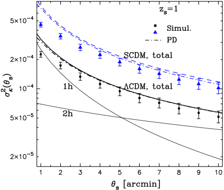
Figure 1: The variance of the convergence field as a function of the top-hat smoothing scale $\theta_{\rm s}$. The solid and dashed lines show the halo model predictions for the SCDM and $\Lambda$CDM models, respectively, with the source redshift $z_{\rm s}=1$. The square and triangle symbols are results from ray-tracing simulation, with error bars giving the sample variance for a survey area of $25~{}{\rm degree}^{2}$, calculated from the simulation data of Hamana & Mellier (2001). The thin solid lines are the 1-halo and 2-halo contributions for the $\Lambda$CDM model. The dot-dashed lines are the predictions from the Peacock-Dodds fitting formula.

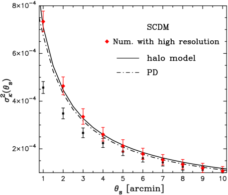
Figure 2: Shown is the comparison of the high resolution simulation results (diamond symbol) of $\sigma_{\kappa}^{2}$ (Jain et al.2000) with the results (square) of lower resolution data (Hamana & Mellier 2001) for SCDM. The latter data is mainly used for the comparisons with model predictions in this paper as explained in the text. The solid and dot-dashed lines are the predictions of the halo model and PD, respectively, as in Figure 1. Note that the error bars for the JSW data correspond to the sample variance for a survey area of $2.8\times 2.8~{}{\rm degree}^{2}$.

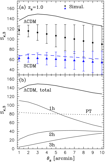
Figure 3: The skewness parameter as a function of $\theta_{\rm s}$ as in Figure 1. The upper panel shows a comparison of the halo model predictions with the simulation results, while the lower panel shows contributions from the 1-halo, 2-halo and 3-halo terms for the $\Lambda$CDM model. For comparison, the dotted line in the lower panel shows the result predicted by the second-order perturbation theory.

Figure 1 plots the convergence variance as a function of the top-hat smoothing scale for the SCDM ($\Omega_{\rm m0}=1$, $h=0.5$, $\sigma_{8}=0.6$) and $\Lambda$CDM ($\Omega_{\rm m0}=0.3$, $\Omega_{\lambda 0}=0.7$, $h=0.7$, $\sigma_{8}=0.9$) models. We fix $z_{\rm s}=1$ for the source galaxy redshift. For the linear matter power spectrum used in the calculation, we employ a scale invariant spectrum of the primordial fluctuations with the BBKS transfer function [Bardeen et al. 1986]. The solid and dashed lines show the results of our halo model for the $\Lambda$CDM and SCDM models, respectively, while the dot-dashed lines are the predictions of using the Peacock & Dodds (1996; hereafter PD) fitting formula for the nonlinear power spectra. The 1-halo and 2-halo contributions are shown by the thin solid lines for $\Lambda$CDM, and one can see that the variance arises mainly from the 1-halo term on angular scales of $\theta_{\rm s}\lower 2.15277pt\hbox{$\;\buildrel<\over{\sim}\;$}5^{\prime}$, where nonlinear structures play important role to the weak lensing statistics (see, e.g. Jain & Seljak 1997). The symbols with error bars are the ray-tracing simulation results, where the error in each bin denotes the sample variance for a weak lensing survey with an area of $25~{}{\rm degree}^{2}$. The ray-tracing simulation builds on an N-body simulation based on the particle-mesh (PM) code and has been kindly made available to us by T. Hamana (for details see Hamana & Mellier 2001; hereafter HM).

It is clear from Figure 1 that the halo model predictions are in good agreements with the PD results as well as with the simulation results for both the $\Lambda$CDM and SCDM models. We have indeed confirmed that for all cosmological models we consider in this paper the halo model can reproduce the PD results for $\sigma_{\kappa}^{2}(\theta_{\rm s})$ within $\sim 5\%$ accuracy on angular scales of interest. This success at the two-point level is partly due to our choice (5) of the concentration parameter for the NFW profile. However, there are slight differences between the predictions and the numerical results on small angular scales $\theta_{\rm s}\lower 2.15277pt\hbox{$\;\buildrel<\over{\sim}\;$}3^{\prime}$. This is possibly due to the lack of the numerical resolution of the ray-tracing data, because the higher resolution simulation used by JSW yields more power on such small scales, which gives a better match to the theoretical predictions, as explicitly shown in Figure 2 (see also discussions in Taruya et al. 2002 for the resolution of the HM data). We prefer to use the HM data for comparison to our model predictions because we can use 40 realizations of simulation data with $25~{}{\rm degree}^{2}$ for each CDM model in order to correctly estimate the sample variance. Having an adequate number of the realizations is crucial to study the higher-order moments especially on large angular scales, $\theta_{\rm s}\lower 2.15277pt\hbox{$\;\buildrel>\over{\sim}\;$}5^{\prime}$, since the higher moments are more sensitive to sample variance.

In analogy with the second moment, the third-order moment of the filtered convergence field can be expressed in terms of the bispectrum as

$$\langle{\kappa^{3}(\theta_{\rm s})}\rangle=\int\!\!d\chi W^{3}(\chi,\chi_{\rm s})d_{A}^{-4}(\chi)\int\!\!\frac{d^{2}\mbox{{\it\boldmath$l$}}_{1}}{(2\pi)^{2}}\frac{d^{2}\mbox{{\it\boldmath$l$}}_{2}}{(2\pi)^{2}}B\left(\mbox{{\it\boldmath$k$}}_{1},\mbox{{\it\boldmath$k$}}_{2},-\mbox{{\it\boldmath$k$}}_{12}\right)F(l_{1})F(l_{2})F(l_{12}),$$ (25)

where $\mbox{{\it\boldmath$k$}}_{i}=\mbox{{\it\boldmath$l$}}_{i}/d_{A}(\chi)$ and $B$ for the halo model is given by equation (11). We explicitly write down the 1-halo contribution to $\langle{\kappa^{3}}\rangle$:

$$\langle{\kappa^{3}(\theta_{\rm s})}\rangle^{1h}=\int\!\!d\chi W^{3}(\chi,\chi_{\rm s})d_{A}^{-4}(\chi)\int\!\!dM\frac{dn}{dM}\left(\frac{M}{\bar{\rho}_{0}}\right)^{3}\int\!\!\frac{d^{2}\mbox{{\it\boldmath$l$}}_{1}}{(2\pi)^{2}}\frac{d^{2}\mbox{{\it\boldmath$l$}}_{2}}{(2\pi)^{2}}y(l_{1},M)y(l_{2},M)y(l_{12},M)F(l_{1})F(l_{2})F(l_{12}).$$ (26)

Although the Fourier transform of the NFW profile, $y(k,M)$, is given as a function of the three-dimensional wavenumber $k$, we will often use $l$ for the argument of $y(k,M)$ according to the relation of $k=l/d_{A}(\chi)$ for simplicity. To obtain $\langle{\kappa^{3}(\theta_{\rm s})}\rangle^{1h}$, we need to perform a 5-dimensional numerical integration, since we can eliminate one angular integration using statistical symmetry. The convergence skewness parameter is defined by

$$S_{\kappa,3}(\theta_{\rm s})\equiv\frac{\langle{\kappa^{3}(\theta_{\rm s})}\rangle}{\sigma^{4}_{\kappa}(\theta_{\rm s})}.$$ (27)

This form is motivated by the fact that in perturbation theory both the numerator and denominator in equation (27) scale as $\sim\delta_{1}^{4}$, where $\delta_{1}$ is the linear solution for the density fluctuation field. Hence the skewness becomes almost independent of the power spectrum normalization $\sigma_{8}$, giving roughly a dependence as $S_{\kappa,3}\propto\Omega_{\rm m0}^{-1}$ through the dependences of the angular distances and the growth rate of the fluctuations (Bernardeau et al. 1997). In the results shown below, we use the halo model self-consistently to compute $\sigma_{\kappa}(\theta_{\rm s})$ in the denominator of $S_{\kappa,3}$. Since our halo model can reproduce the PD results for $\sigma_{\kappa}^{2}$ within $5\%$ accuracy, this does not significantly affect our results for the skewness or kurtosis parameters.

Figure 3 plots the convergence skewness parameter as a function of the smoothing scale as in Figure 1. It is clear from the upper panel that the halo model prediction agrees well with the simulation result for SCDM over all scales. For the $\Lambda$CDM model our model slightly overestimates the simulation result on small scales. Among the possible reasons for this discrepancy, one is that the HM simulation result may underestimate the true value of $S_{\kappa,3}$ due to a lack of numerical resolution as explained in Figure 2. As shown in the lower right panel of Figure 18 in JSW, the high-resolution N-body simulations yields $S_{\kappa,3}\approx 140$ for $\Lambda$CDM on small angular scales, which gives a better match to our halo model prediction. However, the precise value of $S_{\kappa,3}$ for the $\Lambda$CDM model in numerical simulations is still perhaps an open issue. Independent ray-tracing simulation performed by White & Hu (2000; hereafter WH) indicate $S_{\kappa,3}\approx 110$ around $\theta_{\rm s}=4^{\prime}$. We found that an important difference in the WH simulations is the values of cosmological parameters, since they use $\sigma_{8}=1.2$ and $\Gamma=0.2$ for the $\Lambda$CDM model, whereas JSW and HM used $\sigma_{8}=0.9$ and $\Gamma=0.21$. For the cosmological models used in WH, our halo model predicts a $\sim 15\%$ decrease of $S_{\kappa,3}$ at $\theta_{\rm s}\leq 5^{\prime}$ compared with Figure 3 and the resulting $S_{\kappa,3}$ is then marginally consistent with the result shown in Figure 9 of WH on the angular scales we have considered. This is probably due to the increase of $\sigma_{8}$ from $0.9$ to $1.2$, which affects the skewness in a complex way since nonlinear contributions are significant in both its numerator and denominator. Thus on these small scales the expectation from perturbation theory that $S_{\kappa,3}$ is independent of $\sigma_{8}$ is not exactly valid. The halo model predicts that the skewness and kurtosis of lensing fields slightly decrease with increasing $\sigma_{8}$ as shown in Figure 17 for the shear kurtosis. Another difference between the N-body simulation codes used in HM, WH and JSW is that the JSW data is based on the adaptive particle-particle/particle-mesh (AP³M) N-body simulations (see Jenkins et al. 1998 in more detail), while the HM and WH data are based on the particle-mesh (PM) simulations. The AP³M method is expected to achieve higher resolution than PM method for similar mesh resolution. We were able to use a new high-resolution simulation performed with an AP³M code using $512^{3}$ particles [Hamana 2002] to compute the skewness. The new data gives $S_{\kappa,3}\approx 137$ for $\theta_{\rm s}=1^{\prime}$, which agrees with the halo model result in Figure 3, but we also find $S_{\kappa,3}\approx 125$ for $\theta_{\rm s}=4^{\prime}$, a value higher than the simulation result shown in Figure 3, but still lower than the halo model prediction at the 1-$\sigma$ level. Finally, we note that $S_{\kappa,3}$ has a stronger dependence on $\Omega_{\rm m0}$ with decreasing $\Omega_{\rm m0}$; for example, slight decrease of $\Delta\Omega_{\rm m0}=-0.05$ leads to a significant change of $\Delta S_{\kappa,3}\approx 21$ at $\theta_{\rm s}=1^{\prime}$ for flat CDM models with the $\Lambda$CDM model taken to be the fiducial model, while the skewness for the SCDM model is almost unchanged with $\Delta S_{\kappa,3}\approx 1$. These scalings are roughly consistent with the expectation scaling $S_{\kappa,3}\propto\Omega_{\rm m0}^{-1}$. Hence, the discrepancy between our model and the simulation result for the $\Lambda$CDM model corresponds to a relatively small change in $\Omega_{\rm m0}$.

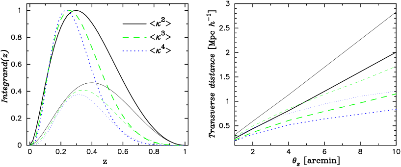
Figure 4: The left panel shows the dependences of the integrand on redshift for the variance (solid line) and the third- (dashed) and forth-order (dotted) moments of the convergence field. The source redshift and the filtering scale are $z_{s}=1$ and $\theta_{\rm s}=1^{\prime}$. The bold and thin lines are results for the SCDM and $\Lambda$CDM models, respectively, and each curve is normalized by the SCDM value at the peak redshift. The figure shows that compared to the SCDM model, the amplitude of each integrand decreases for $\Lambda$CDM and the peak redshift shifts to higher $z$. In the right panel, we show the comoving transverse distance at the peak redshift of these integrands against the angular smoothing scale.

In the lower panel of Figure 3, the 1-halo, 2-halo and 3-halo contributions to $S_{\kappa,3}$ are separately plotted for $\Lambda$CDM . Notice that, for example, ‘1-halo’ here means the convergence third-order moment in $S_{\kappa,3}$ includes only the 1-halo contribution, but the convergence variance used includes the total contributions from the 1-halo and 2-halo terms. It is apparent that the 1-halo term dominates over all scales shown and, in particular, contributes $\sim 80\%$ of the total at the smallest scale $\theta=1^{\prime}$. This holds for the SCDM model also. The result thus implies that the higher-order moments are more sensitive to massive and rare dark matter halos than the variance [Scoccimarro et al. 2001, Cooray & Hu 2001a, Cooray & Hu 2001b]. The dotted line shows the skewness calculated by perturbation theory for the same $\Lambda$CDM model, and it significantly underestimates $S_{\kappa,3}$, since the weak lensing field on relevant scales is affected by strongly nonlinear gravitational clustering. These features can be more explicitly explained in Figure 4. In the left panel, we plot how the integrand functions for the variance (solid line) and the third- (dashed) and fourth-order (dotted) moments of the convergence field depend on redshift for $z_{s}=1$ and $\theta_{\rm s}=1^{\prime}$. Note that the fourth-order moment is computed using the approximation developed below. The bold and thin lines are the results for the SCDM and $\Lambda$CDM models, respectively, where each curve is normalized by the SCDM value at the peak redshift. One can readily see that the higher-order moments are more sensitive to lower redshift structures and, compared with the result for SCDM, the amplitude of each integrand decreases for $\Lambda$CDM and the peak redshift shifts to higher $z$. The right panel plots the comoving transverse distance at the peak redshift of the integrand function as a function of the smoothing scale $\theta_{\rm s}$, which is defined by $\lambda=d_{A}(z_{\rm peak})\theta_{\rm s}$. Again, the figure clarifies that the higher-order moments are more sensitive to structures on smaller scales; for example, by comparing the solid and dotted lines one finds that the transverse scales for the fourth-order moment are smaller than those for the variance by factors of $0.8$ and $0.4$ at $\theta_{\rm s}=1^{\prime}$ and $10^{\prime}$, respectively

It is worth noting differences between the convergence skewness, the shear three-point correlation function recently proposed in BvWM (see also Bernardeau, Mellier & Van Waerbeke 2002), and the shear kurtosis. As shown in Figure 3, $S_{\kappa,3}$ has a weak dependence on the angular scales as pointed out based on the perturbation theory (Bernardeau et al. 1997), while the shear three-point correlation function has a logarithmically decreasing behavior with decreasing the angular scale as shown in Figure 6 in BvWM. It is likely that their shear three-point function loses useful non-Gaussian information resulting from cancellations between signals caused by the vector-like property of the shear field. An advantage of the shear kurtosis parameter is that it collapses information from the 4-point statistics into a single quantity without being affected by such cancellations. However the kurtosis parameter is a higher-order moment, and so it remains to be seen how its signal-to-noise properties compare with the three-point function of BvWM.

4 The kurtosis of the convergence field

In this section, we develop a useful approximation for fast and accurate evaluations of the convergence kurtosis parameter. In particular, we concentrate on developing approximations for calculating the 1-halo term, $\langle{\kappa^{4}(\theta_{\rm s})}\rangle^{1h}_{c}$, which provides the dominant contribution to the convergence kurtosis on small angular scales. The approximations for the 2-halo and 3-halo terms are presented in Appendix C. Those approximations will be used to develop a method to compute the shear kurtosis in the next section.

4.1 Definition

The connected part of the fourth-order moment of the convergence field is given by

$$\langle{\kappa^{4}(\theta_{\rm s})}\rangle_{c}=\int\!\!d\chi W^{4}(\chi,\chi_{s})d_{A}^{-6}\int\!\!\frac{d^{2}\mbox{{\it\boldmath$l$}}_{1}}{(2\pi)^{2}}\frac{d^{2}\mbox{{\it\boldmath$l$}}_{2}}{(2\pi)^{2}}\frac{d^{2}\mbox{{\it\boldmath$l$}}_{3}}{(2\pi)^{2}}T(\mbox{{\it\boldmath$k$}}_{1},\mbox{{\it\boldmath$k$}}_{2},\mbox{{\it\boldmath$k$}}_{3},-\mbox{{\it\boldmath$k$}}_{123})F(l_{1})F(l_{2})F(l_{3})F(l_{123}),$$ (28)

where $\mbox{{\it\boldmath$k$}}_{i}=\mbox{{\it\boldmath$l$}}_{i}/d_{A}(\chi)$ and the trispectrum is given by equation (13) within the framework of the halo model. From the results of the convergence skewness, it is expected that the most important contribution to the fourth-order moment is the 1-halo term on angular scales of interest. The 1-halo term is given by

$$\langle{\kappa^{4}(\theta_{\rm s})}\rangle_{c}^{1h} = \int\!\!d\chi W^{4}(\chi)d_{A}^{-6}\int\!\!dM\frac{dn}{dM}\left(\frac{M}{\bar{\rho}_{0}}\right)^{4}\int\!\!\frac{d^{2}\mbox{{\it\boldmath$l$}}_{1}}{(2\pi)^{2}}\frac{d^{2}\mbox{{\it\boldmath$l$}}_{2}}{(2\pi)^{2}}\frac{d^{2}\mbox{{\it\boldmath$l$}}_{3}}{(2\pi)^{2}}y(l_{1},M)y(l_{2},M)y(l_{3},M)y(l_{123},M)$$ (29)

$$\hskip 260.0004pt\times F(l_{1})F(l_{2})F(l_{3})F(l_{123}).$$

Hence, to obtain $\langle{\kappa^{4}(\theta_{\rm s})}\rangle^{1h}_{c}$, we have to perform at least a 7 dimensional numerical integration, even after we eliminate one angular integration of $\mbox{{\it\boldmath$l$}}_{i}$ using statistical symmetry. Direct integration is not suitable for our final purpose of evaluating the dependence on cosmological parameters, which requires lots of computations in parameter space. We therefore explore an approximation for calculating $\langle{\kappa^{4}}\rangle_{c}$ with adequate accuracy and reasonable computational expense.

Motivated by perturbation theory, as for the skewness parameter, we consider the convergence kurtosis parameter defined by

$$S_{\kappa,4}(\theta_{\rm s})\equiv\frac{\langle{\kappa^{4}(\theta_{\rm s})}\rangle_{c}}{\sigma_{\kappa}^{6}(\theta_{\rm s})}.$$ (30)

We use self-consistently the halo model to calculate $\sigma_{\kappa}(\theta_{\rm s})$ in the denominator of $S_{\kappa,4}$. It is expected that $S_{\kappa,4}$ has a dependence roughly given by perturbation theory as $S_{\kappa,4}\propto\Omega_{\rm m0}^{-2}$.

The approximation for calculating $S^{1h}_{\kappa,4}$ developed below allows us to simplify the three-dimensional angular integrations of $d^{2}\mbox{{\it\boldmath$l$}}_{1}d^{2}\mbox{{\it\boldmath$l$}}_{2}d^{2}\mbox{{\it\boldmath$l$}}_{3}$ in equation (29), whereby we can obtain $\langle{\kappa^{4}(\theta_{\rm s})}\rangle^{1h}_{c}$ by a 5-dimensional numerical integration instead of the original 8-dimensional one.

4.2 Quadrilateral configuration dependence

Equation (29) shows that, although the integrand function of $\langle{\kappa^{4}(\theta_{\rm s})}\rangle^{1h}_{c}$ does depend on quadrilateral configuration with four sides $\mbox{{\it\boldmath$l$}}_{1}$, $\mbox{{\it\boldmath$l$}}_{2}$, $\mbox{{\it\boldmath$l$}}_{3}$ and $\mbox{{\it\boldmath$l$}}_{4}(=-\mbox{{\it\boldmath$l$}}_{123})$ in Fourier space, the angular dependences of $\mbox{{\it\boldmath$l$}}_{i}$ appear only via $\mbox{{\it\boldmath$l$}}_{123}$ in $y(l_{123},M)$ and $F(l_{123})$ as a result of the spherical symmetry of the NFW profile. Because of statistical symmetry, without loss of generality we can express any configurations in terms of 5 parameters; three side lengths of $l_{1}$, $l_{2}$ and $l_{3}$ and two angles $\Phi_{2}$ and $\Phi_{3}$, where $\Phi_{2}$ is angle between $l_{1}$ and $l_{2}$ and $\Phi_{3}$ angle between $l_{12}$ and $l_{3}$. The side length $l_{123}$ can then be expressed as

$$l_{123}=\sqrt{l_{12}^{2}+l_{3}^{2}-2l_{12}l_{3}\cos\Phi_{3}},$$ (31)

with $l_{12}=(l_{1}^{2}+l_{2}^{2}-2l_{1}l_{2}\cos\Phi_{2})^{1/2}$. Note that the volume element (29) of integration can be rewritten, after performing one of the angular integrals, as $d^{2}\mbox{{\it\boldmath$l$}}_{1}d^{2}\mbox{{\it\boldmath$l$}}_{2}d^{2}\mbox{{\it\boldmath$l$}}_{3}=(2\pi)l_{1}dl_{1}l_{2}dl_{2}l_{3}dl_{3}d\Phi_{2}d\Phi_{3}$.

4.3 Approximation for the integration of the top-hat filter function

First, we consider an approximation for the integration of the top-hat filter function (23) motivated by Appendix A in Bernardeau (1994), where the geometrical properties of the integration of products of the three-dimensional top-hat window function are derived. In Appendix B we prove the following identity for the integration of products of top-hat kernels:

$$\int\!\!\frac{d^{2}\mbox{{\it\boldmath$l$}}_{1}}{(2\pi)^{2}}\frac{d^{2}\mbox{{\it\boldmath$l$}}_{2}}{(2\pi)^{2}}\frac{d^{2}\mbox{{\it\boldmath$l$}}_{3}}{(2\pi)^{2}}F(l_{1})F(l_{2})F(l_{3})F(l_{123})=\int\!\!\prod_{i=1}^{3}\frac{l_{i}dl_{i}}{2\pi}F^{2}(l_{i}).$$ (32)

The result above cannot be applied exactly to simplify equation (29) because of the $y(l_{123})$ term. We therefore use the following replacement for the filter function $F(l_{123})$ in equation (29) as an approximation to be tested:

$$F(l_{123})\approx F(l_{1})F(l_{2})F(l_{3}).$$ (33)

The corresponding approximation for the three-dimensional window function is used in Scoccimarro et al. (2001) for the study of the skewness and kurtosis parameters of the three-dimensional density field. It is worth noting that this approximation indeed becomes exact if $y(l,M)=\rm{constant}$ in equation (29). Hence, to the extent that the regime $y(l,M)\approx 1$ at $l\lower 2.15277pt\hbox{$\;\buildrel<\over{\sim}\;$}d_{A}(\chi)c/r_{\rm vir}$ provides the main contribution to $\langle{\kappa^{4}(\theta_{\rm s})}\rangle_{c}^{1h}$ for a given $M$ and $z$, it is reasonable to expect that the replacement (33) is a good approximation for realistic density profiles.

4.4 Approximation for the convergence skewness

Given the approximation (33), the next problem we consider is to explore an approximation to describe the configuration dependence of $y(l_{123},M)$ in a way that allows us to evaluate the angular integrations with respect to $\Phi_{2}$ and $\Phi_{3}$ in equation (29).

For this purpose, let us begin by considering an approximation for calculating the 1-halo term in the convergence third-order moment, $\langle{\kappa^{3}}\rangle^{1h}$. This is because the accuracy of our approximation for $\langle{\kappa^{3}}\rangle^{1h}$ can be tested by comparing the prediction with the true value obtained by the direct integration, and then it can be extended to the calculation of the fourth-order moment. The dependence on the triangle configuration appears via $l_{12}$ in $y(l_{12},M)$ with $l_{12}=(l_{1}^{2}+l_{2}^{2}-2l_{1}l_{2}\cos\Phi_{2})^{1/2}$. We propose a method to expand $y(l_{12})$ around a fiducial triangle configuration with a fixed $\Phi_{2}$ in analogy with the Taylor expansion of $y(l_{12})$ with respect to $\Phi_{2}$, whereby we can analytically perform the angular integrations of $\mbox{{\it\boldmath$l$}}_{i}$ in equation (26). The critical question that arises is: which fiducial configuration is appropriate for the expansion? This can be answered by using the halo model analysis of Cooray & Hu (2001a) for the convergence bispectrum, which is part of the integrand of $\langle{\kappa^{3}}\rangle$. Figure 7 in their paper explicitly illustrates the configuration dependence of the bispectrum and implies that the main contribution to $\langle{\kappa^{3}(\theta_{\rm s})}\rangle$ arises from equilateral triangle configurations with $l_{1}=l_{2}=l_{12}$. Hence, it will be reasonable to take a prescription that the fiducial configuration contains equilateral triangle configurations when $l_{1}=l_{2}$. This holds for $\Phi_{2}=\pi/3$. We thus propose the following approximation for calculating $\langle{\kappa^{3}(\theta_{\rm s})}\rangle^{1h}$ combined with the approximation (33):

$$\langle{\kappa^{3}(\theta_{\rm s})}\rangle^{1h}\approx\int\!\!d\chi W^{3}(\chi,\chi_{\rm s})d_{A}^{-4}\int\!\!dM\frac{dn}{dM}\left(\frac{M}{\bar{\rho}_{0}}\right)^{3}\int\!\!\frac{l_{1}dl_{1}}{2\pi}\frac{l_{2}dl_{2}}{2\pi}y(l_{1})y(l_{2})y(\tilde{l}_{12})F^{2}(l_{1})F^{2}(l_{2}),$$ (34)

with $\tilde{l}_{12}=(l_{1}^{2}+l_{2}^{2}-l_{1}l_{2})^{1/2}$. Note that $\tilde{l}_{12}=l_{1}=l_{2}$ when $l_{1}=l_{2}$, so that the dimension of integration is reduced from 5 to 4 in equation (26). Like the Taylor expansion, one can include higher-order corrections arising from the expansion of $y(l_{12},M)$ at the order of $O(\Phi_{2}-\pi/3)$. We find that the zeroth-order approximation (34) works remarkably well as shown below.

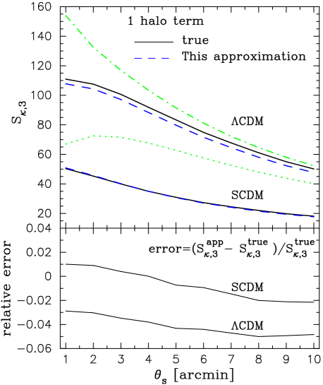
Figure 5: Comparison of our approximation for the 1-halo term of convergence skewness parameter with direct integration values for the SCDM and $\Lambda$CDM models. The solid lines are the direct integration values, while the dashed lines show the results of approximation (34). For comparison, we also show the results calculated using other approximations for $\Lambda$CDM: the dot-dashed and dotted lines are computed using the replacements of $y(l_{12},M)\approx y(l_{1},M)$ and $y(l_{12})\approx y(l_{1},M)y(l_{2},M)$, respectively, for the integration. In the lower panel, the relative errors of our approximation are shown for the two models.

Figure 5 demonstrates the accuracy of our approximation (34) for the 1-halo term of the convergence skewness by comparing the predictions with the direct integration results of equation (26) for the SCDM and $\Lambda$CDM models. The approximation is very accurate, as its relative accuracy is better than $5\%$ over all angular scales for both models. For comparison, the dotted and dot-dashed lines show the results of using other possible approximations for $\Lambda$CDM, where we used the replacements of $y(l_{12},M)=y(l_{1},M)y(l_{2},M)$ or $y(l_{12},M)=y(l_{1},M)$ in equation (26), respectively, in addition to the approximation (33) for the filter function. The former approximation is motivated on the analogy of equation (33), while the latter is indeed used by Scoccimarro et al. (2001) for calculations of the skewness and kurtosis parameters of the three-dimensional density field. It is clear that the approximation of $y(l_{12})=y(l_{1})$ overestimates the value of $S_{\kappa,3}^{1h}$ (see also Cooray & Hu 2001a) and the discrepancy is larger on smaller scales. In more detail, it overestimates $S_{\kappa,3}^{1h}$ by $\sim 40\%$ at $\theta_{\rm s}=1^{\prime}$. The approximation $y(l_{12},M)=y(l_{1},M)y(l_{2},M)$ underestimates the skewness, since $y(l,M)\leq 1$, and yields $S_{\kappa,3}^{1h}$ smaller by $\sim 60\%$ than the correct value. Hence, we cannot use these approximations to predict the higher-order moments of weak lensing fields with sufficient accuracy for our purpose.

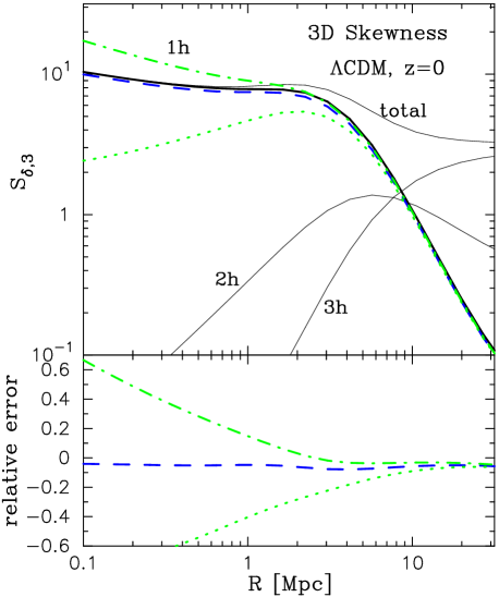
Figure 6: The skewness parameter of the three-dimensional density field, $S_{\delta,3}=\langle{\delta^{3}}\rangle/\langle{\delta^{2}}\rangle^{2}$, as a function of the top-hat smoothing scale, $R$ (Mpc), for the $\Lambda$CDM model at $z=0$. We demonstrate the performance of our approximation for the 1-halo contribution as shown in Figure 5. The dotted and dot-dashed lines show other approximations for the 1-halo term used in the figure, as in Figure 5. The thin lines are the 2-halo, 3-halo and total contributions.

It is straightforward to apply our approximation to evaluations of the skewness parameter of the three-dimensional density field, $S_{\delta,3}\equiv\langle{\delta^{3}}\rangle/\langle{\delta^{2}}\rangle^{2}$, which is relevant for surveys of galaxies clustering (e.g., see Scoccimarro et al. 2001). Figure 6 plots the result against the three-dimensional smoothing scale $R$ (Mpc) for the $\Lambda$CDM model and $z=0$ as shown in Figure 5. Note that we have used the three-dimensional top-hat filter function, and equation (33) can be used as an approximation for the kernel. It is clear that our approximation again works well, implying that it will be useful for efficiently exploring parameter space for constraining cosmological parameters from $S_{\delta,3}$ measurements down to very small scales. The issue of the small scale behavior of higher-order moments is somewhat an open question since results from numerical simulations are not yet reliable for scales below 1 Mpc. The results shown in this paper for the third and fourth-order moment are encouraging. To the extent that the current halo model describes clustering accurately, we have tractable analytical means of predicting higher-order clustering statistics extending to very small scales.

4.5 Approximation for the convergence kurtosis

Figure 7: The sketch of the fiducial 4-point configuration used in the approximation (35) for calculation the convergence fourth-order moment. The two angles $\Phi_{2}$ and $\Phi_{3}$ are set to be $\pi/2$ and $\pi/4$, respectively, but the side length parameters $l_{1}$, $l_{2}$ and $l_{3}$ are treated as variables.

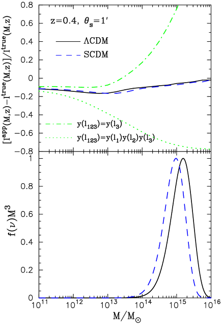
Figure 8: Shown is the accuracy of our approximation (36) for the integrand function ${\cal I}(M,z)$ for the 1-halo term of the convergence fourth-order moment. For the $\Lambda$CDM and SCDM models, the relative errors defined by $({\cal I}^{\rm app}-{\cal I}^{\rm true})/{\cal I}^{\rm true}$ are plotted as the solid and dashed lines, respectively, as a function of halo mass $M$. We here fix $z=0.4$ and $\theta_{\rm s}=1^{\prime}$ for the lens redshift and the smoothing scale. For comparison, the dotted and dot-dashed lines show the results of using other approximations as in Figure 5 (see text for more details). In the lower panel, we plot the mass function weighing, $f(\nu)M^{3}$, in the 1-halo term for the models, where each curve is normalized to give unity at the peak scale.

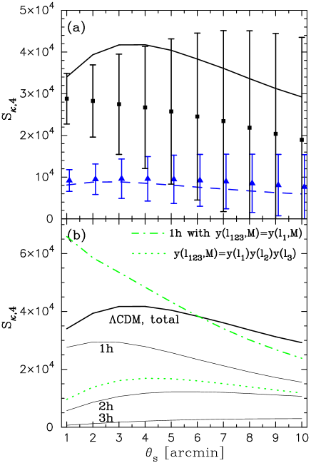
Figure 9: Convergence kurtosis $S_{\kappa,4}$ as a function of the smoothing scale as in Figure 3. The square and triangle symbols with error bars are the simulation results for the $\Lambda$CDM and SCDM models, respectively, while the solid and dashed lines denote our model predictions. For illustration, we slightly shift the simulation result for SCDM along the x-axis. The thin solid lines in the lower panel are the 1-halo, 2-halo and 3-halo contributions for the $\Lambda$CDM model. For comparison, the dotted and dot-dashed lines are the results of other approximations for the 1-halo term as in Figure 8.

Based on the above success of our approximation for the skewness parameter, we extend it to develop an approximation for the 1-halo term of the convergence fourth-order moment, $\langle{\kappa^{4}}\rangle^{1h}_{c}$. The problem is to consider an efficient expansion of $y(l_{123},M)$ in equation (29) with respect to the two angles $\Phi_{2}$ and $\Phi_{3}$, such that we can analytically perform the two-dimensional angular integrations of $\Phi_{2}$ and $\Phi_{3}$. In the same spirit as the approximation (34), we choose the fiducial configuration with $l_{1}=l_{2}=l_{3}=l_{123}$, because we believe, in analogy with the skewness, that the trispectrum with such configurations produces the main contribution to the fourth-order moment. For the kurtosis, we need to make additional choices for the angles $\Phi_{2}$ and $\Phi_{3}$; we simply set $\Phi_{2}=\pi/2$ and $\Phi_{3}=\pi/4$, which implies a square shaped configuration when $l_{1}=l_{2}=l_{3}$. The sketch in Figure 7 illustrates the fiducial 4-point configuration. Applying the above approximation to equation (29) gives

$$\langle{\kappa^{4}(\theta_{\rm s})}\rangle_{c}^{1h}\approx\int\!\!d\chi W^{4}(\chi,\chi_{\rm s})d_{A}^{-6}\int\!\!dM\frac{dn}{dM}\left(\frac{M}{\bar{\rho}_{0}}\right)^{4}{\cal I}(M,z;\theta_{\rm s}),$$ (35)

with

$${\cal I}(M,z;\theta_{\rm s})\equiv\int\!\!\prod_{i=1}^{3}\frac{l_{i}dl_{i}}{2\pi}y(l_{1},M)y(l_{2},M)y(l_{3},M)y(\tilde{l}_{123},M)F^{2}(l_{1})F^{2}(l_{2})F^{2}(l_{3}).$$ (36)

where $\tilde{l}_{123}=(\tilde{l}_{12}^{2}+l_{3}^{2}-\sqrt{2}\tilde{l}_{12}l_{3})^{1/2}$ with $\tilde{l}_{12}=(l_{1}^{2}+l_{2}^{2})^{1/2}$. Consequently, to obtain $\langle{\kappa^{4}}\rangle^{1h}_{c}$, we need to perform a 5-dimensional numerical integration, which requires much less computational time compared with the original 7-dimensional integration of equation (29).

Figure 8 demonstrates the accuracy of our approximation (35). The approximate result for ${\cal I}(M,z)$ is compared with the direct integration value, plotted against halo mass $M$ for the $\Lambda$CDM model. The lens redshift is $z=0.4$ and smoothing scale $\theta_{\rm s}=1^{\prime}$. Note that for fixed $z$ and $M$ we can directly compute ${\cal I}(M,z)$ by evaluating the 5-dimensional integral. It is also worth noting that $z=0.4$ is chosen because it is close to the peak of the lensing weight function $W(\chi,\chi_{\rm s})$ for source redshift $z_{\rm s}=1$. The figure clearly shows that for both SCDM and $\Lambda$CDM models our approximation can reproduce ${\cal I}(M,z)$ within $10\%$ accuracy on mass scales of $10^{14}M_{\odot}\lower 2.15277pt\hbox{$\;\buildrel<\over{\sim}\;$}M\lower 2.15277pt\hbox{$\;\buildrel<\over{\sim}\;$}10^{16}M_{\odot}$, which provide the dominant contributions to the kurtosis parameter on relevant angular scales as shown in Figure 13. The approximation works better for more massive halos.

To estimate the final accuracy of our approximation to $\langle{\kappa^{4}}\rangle_{c}^{1h}$, we further need to take into account the lens weighting, $W^{4}(\chi,\chi_{\rm s})d^{-6}_{A}$, as well as the weighting of mass function, $f(\nu,z)M^{3}$, in equation (35). Since the lens weighting gives a smooth redshift dependence, we here consider the weighing of mass function. The lower panel in Figure 8 plots $f(\nu,z)M^{3}$ at $z=0.4$ against $M$, where each curve is normalized to give unity at the peak mass scale. Accounting for the weighting of $f(\nu)M^{3}$, we find that the accuracy of our approximation is about $9\%$ and $8\%$ for SCDM and $\Lambda$CDM models at $\theta_{\rm s}=1^{\prime}$ and $z=0.4$. Our approximation works better for the larger smoothing scales, where more massive halos contribute to $\langle{\kappa^{4}}\rangle^{1h}_{c}$ (see Figure 13). From these results, we are confident that our approximation can predict the 1-halo term within $\sim 10\%$ accuracy at most on relevant scales, although we should bear in mind that the approximation has a trend to underestimate the true value. The figure also shows the results from other possible approximations for $\Lambda$CDM , as in Figure 5, where we have used the replacements of $y(l_{123})=y(l_{1})y(l_{2})y(l_{3})$ (dotted line) and $y(l_{123})=y(l_{3})$ (dot-dashed line) (Scoccimarro et al. 2001). These approximations overestimate or underestimate ${\cal I}(M,z)$ by $62\%$ or $70\%$, respectively, and become worse at more massive mass scales, and thus are not accurate enough for our purpose.

Similarly, we can construct approximations for the 2-halo and 3-halo terms to predict a total power of the convergence kurtosis. The explicit forms of the approximations used are presented in Appendix C. We have confirmed that these approximations are adequately accurate (see Scoccimarro et al. 2001 for similar discussions on the skewness and kurtosis of the three-dimensional density field). As explained below, in this paper we ignore the 4-halo contribution which is likely to have a negligible contribution on the angular scales we have considered (see Cooray & Hu 2001b for the trispectrum).

We can now compare our model predictions of the convergence kurtosis parameter with the simulation results. Figure 9 plots the result as in Figure 3. It is apparent that our halo model predictions are in good agreements with the simulation results as for the skewness case. One caveat we should bear in mind is again that the simulation result for $\Lambda$CDM is likely to underestimate $S_{\kappa,4}$ because of the reasons given for Figure 3. We have confirmed this by using new high-resolution simulation data provided by Hamana (2002). We obtained $S_{\kappa,4}\approx 4\times 10^{4}$ at $\theta_{\rm s}=1^{\prime}$ for $\Lambda$CDM, which gives a better match to our model prediction. The main cosmological implication of this figure is that there are still significant differences between SCDM and $\Lambda$CDM models on small scales of $\theta_{\rm s}\lower 2.15277pt\hbox{$\;\buildrel<\over{\sim}\;$}2^{\prime}$, although the sampling errors corresponding to a survey area of $25{\rm~{}degree}^{2}$ become larger compared with the skewness case.

The lower panel of Figure 9 plots the 1-halo, 2-halo and 3-halo contributions for $\Lambda$CDM. It is clear that the 1-halo term gives the dominant contribution over the scales considered; the 2-halo is marginally important on larger scales of $\theta_{\rm s}\lower 2.15277pt\hbox{$\;\buildrel>\over{\sim}\;$}5^{\prime}$ and the 3-halo makes only a small contribution. More explicitly, these terms provide $82\%$, $16\%$ and $2\%$ of the contributions to the total kurtosis at $\theta_{\rm s}=1^{\prime}$; $53\%$, $37\%$ and $10\%$ at $\theta_{\rm s}=10^{\prime}$, respectively. These results validate our expectation that the 4-halo term is negligible on small angular scales $\theta_{\rm s}\lower 2.15277pt\hbox{$\;\buildrel<\over{\sim}\;$}5^{\prime}$, and even for larger scales it is likely to have contributions smaller than $10\%$. The 4-halo term is difficult to evaluate by numerical integration because of the oscillatory shape of the perturbation theory trispectrum, resulting from its dependences on the interior angles of the 4-point configuration.

5 Approximation for the shear kurtosis

Based on the results shown in the preceding section, we develop an approximate method for calculating the shear kurtosis, which is the main purpose of this paper.

The connected fourth-order moment of the filtered shear field can be expressed in terms of the convergence trispectrum as

$$\langle{\gamma_{1}^{4}(\theta_{\rm s})}\rangle_{c}=\int\!\!\prod_{i=1}^{4}\frac{d^{2}\mbox{{\it\boldmath$l$}}_{i}}{(2\pi)^{2}}\cos 2\phi_{l_{i}}F(l_{i})T_{\kappa}(\mbox{{\it\boldmath$l$}}_{1},\mbox{{\it\boldmath$l$}}_{2},\mbox{{\it\boldmath$l$}}_{3},\mbox{{\it\boldmath$l$}}_{4})(2\pi)^{2}\delta_{D}(\mbox{{\it\boldmath$l$}}_{1234}),$$ (37)

with

$$T_{\kappa}\equiv\int\!\!d\chi W^{4}(\chi,\chi_{\rm s})d_{A}^{-6}T\!\left(\mbox{{\it\boldmath$k$}}_{1},\mbox{{\it\boldmath$k$}}_{2},\mbox{{\it\boldmath$k$}}_{3},\mbox{{\it\boldmath$k$}}_{4}\right),$$ (38)

where $\mbox{{\it\boldmath$k$}}=\mbox{{\it\boldmath$l$}}/d_{A}(\chi)$, $\phi_{l_{i}}$ is defined by $\mbox{{\it\boldmath$l$}}_{i}=l_{i}(\cos\phi_{l_{i}},\sin\phi_{l_{i}})$ and $T_{\kappa}$ is the convergence trispectrum (see Cooray & Hu 2001b). This equation clarifies that the integrand function of $\langle{\gamma_{1}^{4}}\rangle_{c}$ has configuration dependences via the geometrical factors of $\cos 2\phi_{l_{i}}$ in addition to the convergence trispectrum, and we therefore have to consider the 8-dimensional integration. Note that for $\langle{\gamma_{2}^{4}}\rangle_{c}$ the geometrical factor in equation (37) is $\prod_{i=1}^{4}\sin 2\phi_{l_{i}}$, but $\langle{\gamma_{1}^{4}}\rangle_{c}=\langle{\gamma_{2}^{4}}\rangle_{c}$ from statistical symmetry. In comparing equation (37) with equation (29) for $\langle{\kappa^{4}}\rangle_{c}$, the difference is only the geometrical factor $\prod_{i=1}^{4}\cos 2\phi_{l_{i}}$. We therefore expect that the following simple relation

$$\langle{\gamma_{1}^{4}(\theta_{\rm s})}\rangle_{c}\approx f_{g}\langle{\kappa^{4}(\theta_{\rm s})}\rangle_{c},$$ (39)

applies, with a constant factor $f_{g}$. We can derive an upper limit for $f_{g}$ in the following rough manner. From the integrand function of $\langle{\gamma_{1}^{4}}\rangle_{c}$, we consider the angular averaged geometrical function as a function of $l_{1}$, $l_{2}$ and $l_{3}$ defined by

$${\cal G}(l_{1},l_{2},l_{3})=\int\!\!\prod_{i=1}^{3}\frac{d\phi_{l_{i}}}{2\pi}\cos 2\phi_{l_{i}}\cos 2\phi_{l_{123}},$$ (40)

where $\cos\phi_{l_{123}}=-(l_{1}\cos\phi_{l_{1}}+l_{2}\cos\phi_{l_{2}}+l_{3}\cos\phi_{l_{3}})/l_{123}$. The function ${\cal G}$ peaks at $l_{1}=l_{2}=l_{3}$ and approaches zero for $l_{1}\ll l_{2},l_{3}$ or $l_{1}\gg l_{2},l_{3}$ and so on, so that the shear fourth-order moment is suppressed compared to that of the convergence. Hence, the upper limit on $f_{g}$ should be set by the case $l_{1}=l_{2}=l_{3}$: $f_{g}\leq{\cal G}(l,l,l)\approx 5.17\times 10^{-2}$.

Given the relation (39), the shear kurtosis can be expressed in terms of the convergence kurtosis as

$$S_{\gamma,4}(\theta_{\rm s})\equiv\frac{\langle{\gamma_{i}^{4}}\rangle_{c}}{\sigma^{6}_{\gamma}(\theta_{\rm s})}\approx 8f_{g}\frac{\langle{\kappa^{4}(\theta_{\rm s})}\rangle_{c}}{\sigma_{\kappa}^{6}(\theta_{\rm s})}=8f_{g}S_{\kappa,4}(\theta_{\rm s}),$$ (41)

where $\sigma_{\gamma}(\theta_{\rm s})$ is the rms of the filtered shear field defined by $\sigma_{\gamma}(\theta_{\rm s})\equiv\langle{\gamma_{i}^{2}(\theta_{\rm s})}\rangle^{1/2}$ and the factor of $8$ comes from the relation $\langle{\gamma_{i}^{2}}\rangle=\langle{\kappa^{2}}\rangle/2$. Note that the upper limit on $f_{g}$ discussed above corresponds to $S_{\gamma,4}\leq 0.41S_{\kappa,4}$.

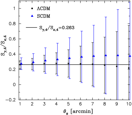
Figure 10: Shown is the ratio of the shear kurtosis parameter to the convergence kurtosis as a function of the smoothing scale. The symbols with error bars are the simulation results for the $\Lambda$CDM and SCDM models as in Figure 1, where the shear kurtosis is obtained by averaging the two kurtosis parameters for $\gamma_{1}$ and $\gamma_{2}$ and the error bar in each bin is properly averaged. The solid line shows the ratio value of $0.263$, which is the average value between the results at $\theta_{\rm s}=1^{\prime}$ for the two models.

Unfortunately, it is difficult to analytically derive the constant factor connecting $S_{\gamma,4}$ and $S_{\kappa,4}$, and we therefore rely on ray-tracing simulations. Figure 10 plots the simulation results for the ratio of $S_{\gamma,4}$ to $S_{\kappa,4}$ as a function of the smoothing scale. Note that we have taken the average of the kurtosis values for the two independent shear fields to obtain $S_{\gamma,4}$; $S_{\gamma,4}\equiv[\langle{\gamma_{1}^{4}}\rangle_{c}/\langle{\gamma_{1}^{2}}\rangle^{3}+\langle{\gamma_{2}^{4}}\rangle_{c}/\langle{\gamma_{2}^{2}}\rangle^{3}]/2$. The figure reveals that, despite the fact that the trispectrum has a strong dependence on cosmological models (leading to a difference greater than $300\%$ between the kurtosis values for the SCDM and $\Lambda$CDM models – see Figure 9), the ratios are similar for the two models. Further, it appears that $S_{\gamma,4}$ is related to $S_{\kappa,4}$ by a constant factor over the angular scales we have considered. The solid line shows the average value of $0.263$ between the results at $\theta_{\rm s}=1^{\prime}$ for the two models, and one can see that the curve reasonably explains the simulation results. In the following, to predict the shear kurtosis parameter, we simply multiply the factor $0.263$ by the convergence kurtosis parameter calculated using the approximations developed in §4.5. Thus we use:

$$S_{\gamma,4}\approx 0.263\ S_{\kappa,4}.$$ (42)

6 RESULTS

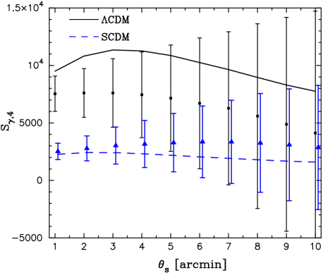
Figure 11: Comparison of our model predictions for the shear kurtosis, $S_{\gamma,4}$, with the simulation results as a function of the smoothing scale. Here, for the simulation result in each bin we take the average between the kurtosis parameters of two shear fields $\gamma_{1}$ and $\gamma_{2}$. For illustration, we slightly shift the simulation result for SCDM along the x-axis.

In Figure 11 we compare our model predictions of the shear kurtosis with the simulation results for the SCDM and $\Lambda$CDM models as in Figure 9. Note that the halo model prediction is calculated from the sum of the 1-halo, 2-halo and 3-halo contributions to the shear fourth-order moment. The result shown in each bin is computed from the average value of the kurtosis parameters for two shear fields, $\gamma_{1}$ and $\gamma_{2}$, as in Figure 10. The figure reveals that our model can well reproduce the simulation results and that there are distinct differences between the shear kurtosis values for the SCDM and $\Lambda$CDM models on small scales of $\theta_{\rm s}\lower 2.15277pt\hbox{$\;\buildrel<\over{\sim}\;$}3^{\prime}$. The range of angular scales with $0.5^{\prime}\lower 2.15277pt\hbox{$\;\buildrel<\over{\sim}\;$}\theta_{\rm s}\lower 2.15277pt\hbox{$\;\buildrel<\over{\sim}\;$}3^{\prime}$ is feasible for making adequate signal-to-noise measurements of top-hat smoothed statistics from lensing survey data (e.g., see Van Waerbeke et al. 2001a). As mentioned in the discussion of Figure 3, the simulation results for $\Lambda$CDM are likely to underestimate $S_{\gamma,4}$ at $\theta_{\rm s}\lower 2.15277pt\hbox{$\;\buildrel<\over{\sim}\;$}3^{\prime}$. We have confirmed that high-resolution simulation [Hamana 2002] does give a better match to our model prediction, but the accurate measurement of fourth-order statistics from numerical data needs further investigation. This uncertainty does not seriously undermine our conclusions about parameter estimation from the shear kurtosis, because it has a strong dependence on $\Omega_{\rm m0}$ for flat $\Lambda$CDM models. E.g. a small change $\Delta\Omega_{\rm m0}=-0.05$ leads to a large change of $\Delta S_{\gamma,4}\approx 3.1\times 10^{3}$ at $\theta_{\rm s}=1^{\prime}$ if one chooses the fiducial model with $\Omega_{\rm m0}=0.3,\Omega_{\lambda 0}=0.7$. On the other hand for variations about the $\Omega_{\rm m0}=1$ model, the result is almost unchanged with $\Delta S_{\gamma,4}\approx 60$. These scalings are approximately consistent with the perturbation theory expectation given by $S_{\gamma,4}\propto\Omega_{\rm m0}^{-2}$ (see also Figure 17 and 18).

Figure 12: Shown is the comparison of our model predictions for the shear kurtosis (upper panel) and the convergence skewness (lower panel) with the results of the JSW simulation data for the $\tau$CDM model, which has $\Omega_{\rm m0}=1.0$, $h=0.5$, $\sigma_{8}=0.6$ and $\Gamma=0.21$.

Figure 13: The dependence of the shear kurtosis on the maximum mass cutoff used in the calculation for the SCDM model. Note the we varied the maximum mass cutoff for evaluations of the shear fourth-order moment and the shear variance, which enter the numerator and denominator of $S_{\gamma,4}$, respectively. From top to bottom, the maximum mass is $10^{16}$, $10^{15}$, $10^{14}$ and $10^{13}M_{\odot}$.

Figure 14: The dependence of the shear kurtosis on the range of lens redshift is plotted. From top to bottom, the lower limit of lens redshift used in the calculation is $0.1$, $0.2$, $0.3$, $0.4$ and $0.5$, while the upper limit is $z=1$.

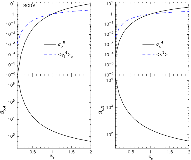
Figure 15: In the left upper panel, the dependences of $\sigma_{\gamma}^{6}(\theta_{\rm s})$ and the shear fourth-order moment on the source galaxy redshift $z_{\rm s}$ are plotted for the SCDM model and $\theta_{\rm s}=1^{\prime}$, while the resulting dependence of the shear kurtosis is shown in the lower left panel. Note that $\sigma_{\gamma}^{6}$ appears in the denominator of $S_{\gamma,4}$. The solid and dashed lines in the upper panel are the results for $\sigma^{6}_{\gamma}$ and $\langle{\gamma_{i}^{4}}\rangle$, respectively, where each curve is normalized by its values for $z_{\rm s}=1$. The right panel is a similar plot for the convergence skewness $S_{\kappa,3}$ given by equation (27); $\sigma_{\kappa}^{4}$ and $\langle{\kappa^{3}}\rangle$ are the denominator and numerator of $S_{\kappa,3}$.

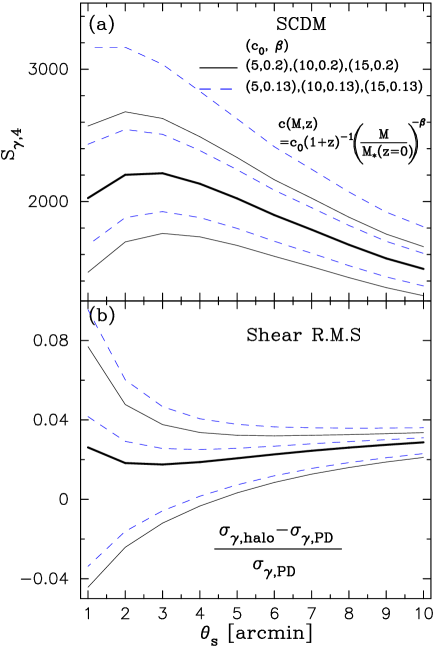
Figure 16: In the upper panel (a), the dependence of the shear kurtosis on variations in the concentration parameter is plotted as a function of the smoothing scale. We consider the concentration parameter expressed in terms of the normalization $c_{0}$ at the present-day nonlinear mass scale, $M_{\star}(z=0)$, and the slope of the mass dependence as $c(M,z)=c_{0}(1+z)\left(M/M_{\star}(z=0)\right)^{-\beta}$. The three solid lines demonstrate the dependences for $(c_{0},\beta)=(5,0.2),(10,0.2),(15,0.2)$ from bottom to top, respectively, while the dashed lines are $(c_{0},\beta)=(5,0.13),(10,0.13),(15,0.13)$. The bold solid line denotes the result for $(c_{0},\beta)=(10,0.2)$, which we have used in this paper. In the lower panel (b), we show the relative differences between the halo model predictions and the PD results for the shear rms. As in the upper panel, the solid lines from bottom to top are the results for $(c_{0},\beta)=(5,0.2),(10,0.2),(15,0.2)$.

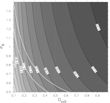
Figure 17: Log contour map of the shear kurtosis parameter $S_{\gamma,4}$ in the $\Omega_{m0}$-$\sigma_{8}$ plane for flat CDM models with $h=0.7$ and $\theta_{\rm s}=1^{\prime}$. Note that the number assigned to each contour is the index value of $a$ which parameterizes the kurtosis as $S_{\gamma}=10^{a}$; each contour is stepped by $\Delta a=0.2$. The two solid curves show the dependence $\sigma_{8}\Omega_{m0}^{0.6}$ that represents typical constraints on the $\Omega_{\rm m0}$-$\sigma_{8}$ plane so far obtained from the two-point shear statistics measurements (the two curves correspond to two different normalizations). It is clear that the curves for the two-point and four-point statistics have different shapes, and would therefore allow for independent determinations of the two parameters.

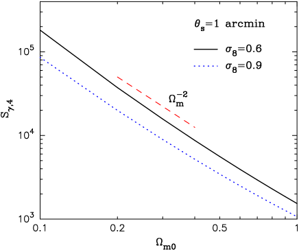
Figure 18: This figure shows slices of the contour plot in Figure 17 with $\sigma_{8}=0.6$ and $0.9$, which explicitly illustrates the dependence of the shear kurtosis on $\Omega_{\rm m0}$. The dashed line shows the dependence $S_{\gamma,4}\propto\Omega_{\rm m0}^{-2}$.

In Figure 12, we show the comparison of our model prediction with the JSW simulation results for the $\tau$CDM model, which has $\Omega_{\rm m0}=1.0$, $h=0.5$, $\sigma_{8}=0.6$ and the shape parameter of $\Gamma=0.21$ (see JSW for more details). Note that the cosmological parameters of the $\tau$CDM model are the same as for SCDM except for the shape parameter ($\Gamma=0.5$ for SCDM). The error in each bin is the sample variance corresponding to a survey area of $\approx 7.84{\rm~{}degree}^{2}$. The purpose of this figure is to illustrate the validity of our model for different cosmological models and the sensitivity of the shear kurtosis to the shape of the matter power spectrum. One can clearly see that our halo model reproduces the simulation results for both the shear kurtosis (upper panel) and the convergence skewness (lower panel). This success may be a surprise, because it has been pointed out in several works (e.g. see Figure 1 in Van Waerbeke et al. 2001b) that the JSW data does not exactly match the amplitude of the convergence variance predicted by the PD formula. The discrepancy may be attributed to the inaccuracy of the PD fitting formula for the nonlinear power spectrum. However it appears that our model can reproduce the simulation results for the statistical measures of weak lensing fields that are chosen to be insensitive to the power spectrum normalization but can pick up the non-Gaussian signals originating from the density field. Figure 12 also shows that the skewness and kurtosis are larger for the $\tau$CDM model compared to the SCDM model. Thus some constraint on the shape of the power spectrum is necessary to use the non-Gaussian statistics for parameter estimation.

So far our halo model calculations have assumed the mass range for the integration as $10^{3}M_{\odot}\leq M\leq 10^{18}M_{\odot}$. Figure 13 plots the dependence of the shear kurtosis on the maximum mass cutoff used in the calculation for the SCDM model. Note that we varied the maximum mass cutoff for evaluations of both the shear variance and the fourth-order shear moment used in the calculation of $S_{\gamma,4}$; the figure shows the resulting dependence of $S_{\gamma,4}$ on the maximum mass cutoff. It is apparent that $S_{\gamma,4}$ is mainly due to massive halos with $M\lower 2.15277pt\hbox{$\;\buildrel>\over{\sim}\;$}10^{14}M_{\odot}$, while less massive halos contribute more on smaller angular scales. More specifically, halos with $M\geq 10^{14}M_{\odot}$ provide $\approx 50\%$ and $\approx 99\%$ contributions to the shear kurtosis at $\theta_{\rm s}=1^{\prime}$ and $10^{\prime}$, respectively.

The dependence of the shear kurtosis on the lens redshift is shown in Figure 14. This figure indicates that the shear kurtosis is sensitive to low redshift structures with $z\lower 2.15277pt\hbox{$\;\buildrel<\over{\sim}\;$}0.4$. Next we examine the origin of the redshift dependence by plotting dependences of the numerator and denominator of the skewness and kurtosis separately.

The upper-left panel in Figure 15 illustrates the dependences of $\sigma_{\gamma}^{6}$ and $\langle{\gamma_{i}^{4}}\rangle_{c}$ on the source galaxy redshift $z_{\rm s}$ for the SCDM model and $\theta_{\rm s}=1^{\prime}$ ($\sigma_{\gamma}^{6}$ and $\langle{\gamma_{i}^{4}}\rangle_{c}$ are the denominator and numerator of $S_{\gamma,4}$, respectively). For comparison, the right panel shows a similar plot for the convergence skewness $S_{\kappa,3}$ (the denominator and numerator of $S_{\kappa,3}$ are $\sigma_{\kappa}^{4}$ and $\langle{\kappa^{3}}\rangle$, respectively). One can see that nonlinear structures at lower redshifts affect the higher-order moments more strongly than the terms with powers of the variance. The lower-left panel plots the resulting dependence of $S_{\gamma,4}$ on the source redshift and reveals that possible variation in the source redshift alters the shear kurtosis. A comparison of the left and right panels shows that the shear kurtosis has a stronger dependence on the source redshift than the convergence skewness. The shear kurtosis increases by a factor of 20 if the source redshift is varied from $0.5$ to $2$, while the convergence skewness varies about by a factor of 7. These results raise the question: what is the best survey strategy to measure the shear kurtosis? Figure 15 suggests that a deeper redshift survey that probes higher-redshift structures loses some non-Gaussian signal due to projection effects. A survey to measure $S_{\gamma,4}$ may be more efficient if it is shallower and covers greater area, provided systematic errors are well understood and the redshift distribution of source galaxies is known. The feasibility of the measurement of non-Gaussian statistics from lensing surveys will be presented in detail elsewhere (Takada et al. 2002).

In Figure 16 we show the effect of varying the concentration parameter of the NFW profile on the shear kurtosis for the SCDM model and $\theta_{\rm s}=1^{\prime}$. The dependence is illustrated by parameterizing the concentration parameter in terms of its normalization at the nonlinear mass scale today and the slope of the mass dependence as $c(M,z)=c_{0}(1+z)^{-1}(M/M_{\ast}(z=0))^{-\beta}$. Here we have again assumed that the redshift dependence is the same as in equation (5) as suggested by the N-body simulations [Bullock et al. 2001]. With fixed $\beta$, a $50\%$ increase or decrease of $c_{0}$ leads to $\sim 30\%$ increase or decrease of $S_{\gamma,4}$. Thus our results would not be strongly affected by varying $c$ to the extent indicated by N-body simulations, which give a dispersion of 0.2 in $\ln c$ (Jing 2000; Bullock et al. 2001; see also Cooray & Hu 2001b for lensing study). On the other hand, the curves with fixed $c_{0}$ and varying $\beta$ reveal that the shallower slope $\beta=0.13$ leads to a larger value of $S_{\gamma,4}$. These results can be explained as follows. The increase of $c_{0}$ for a given $\beta$ or the decrease of $\beta$ for a given $c_{0}$ leads to more concentrated density profiles for halos more massive than the nonlinear mass scale $M_{\ast}$. Since these massive halos dominate the contribution to the shear kurtosis, this has the effect of increasing the kurtosis on the angular scales considered here. An important caveat is that the variations in the concentration parameter simultaneously alter the predictions for the shear variance, $\sigma^{2}_{\gamma}$. The lower panel shows the relative errors of the halo model prediction to the PD results for $\sigma_{\gamma}$. It is clear that our choice (5) for $c(M,z)$ (bold solid line) gives the closest value to the PD result. Furthermore, as we have shown, our model can reproduce the simulation results for the higher-order moments of weak lensing fields. In this regard, therefore, as a prescription for using the halo approach to study the higher-order statistics of weak lensing, it is reasonable to choose the concentration parameter so that it reproduces the PD result for the variance. Conversely, if we employ a different halo profile from NFW, it will probably be necessary to modify our choice (5) for the concentration parameter in order to accurately describe the higher-order statistics.

Finally, in Figure 17 we show the contour plot for $S_{\gamma,4}$ with $\theta_{\rm s}=1^{\prime}$ in the plane of $\Omega_{\rm m0}$ and $\sigma_{8}$ parameters for flat CDM models with $h=0.7$. The number assigned to each contour denotes the value of $\log_{10}S_{\gamma,4}$, in the $\Omega_{\rm m0}-\sigma_{8}$ plane. Clearly, the shear kurtosis is very sensitive to $\Omega_{\rm m0}$ and has a weak dependence on $\sigma_{8}$. For example, the model with $\Omega_{\rm m0}=0.1$ and $\sigma_{8}=0.6$ yields $S_{\gamma,4}=1.72\times 10^{5}$, while the model with $\Omega_{\rm m0}=1.0$ and the same $\sigma_{8}$ leads to $S_{\gamma,4}=1.46\times 10^{3}$. Figure 18 shows slices of the contour plot with $\sigma_{8}=0.6$ and $0.9$, and reveals that the dependence of $S_{\gamma,4}$ on $\Omega_{\rm m0}$ is very close to $S_{\gamma,4}\propto\Omega_{\rm m0}^{-2}$. On the other hand, the two solid lines in Figure 17 show the dependence $\sigma_{8}\Omega_{\rm m0}^{0.6}$, which represents typical constraints obtained from measurements of the two-point statistics of the shear field (each curve is arbitrarily normalized). One can see that these two curves have a very different shape from the contours of $S_{\gamma,4}$; thus measurements of $S_{\gamma,4}$ can break the degeneracy in the determination of $\Omega_{\rm m0}$ and $\sigma_{8}$. Furthermore, they can constrain the dark energy component of the universe if they are combined with the evidence for a flat universe from recent CMB measurements [Netterfield et al. 2001].

7 DISCUSSION AND CONCLUSION

In this paper we have investigated the kurtosis parameter of the cosmic shear field, $S_{\gamma,4}(\equiv\langle{\gamma_{i}^{4}}\rangle_{c}/\langle{\gamma_{i}^{2}}\rangle^{3})$, based on the dark matter halo approach. The two main results revealed in this paper are summarized as follows. First, we have developed a useful approximation for calculating the shear kurtosis, which significantly reduces the computational time and yet provides the shear kurtosis expected within $\sim 10\%$ accuracy over the angular scales $1^{\prime}\leq\theta_{\rm s}\leq 10^{\prime}$. Our model predictions can well match the ray-tracing simulation results for the shear kurtosis as well as for the convergence skewness and kurtosis parameters for the SCDM, $\Lambda$CDM and $\tau$CDM models (see Figure 3, 9, 11 and12). For the $\Lambda$CDM model, the simulation data lie slightly below our predictions. It appears that the numerical results on small scales, especially for the higher-order moments, have not converged at the few percent level of accuracy – this is a subject that merits further investigation. While we have focused on lensing statistics in this paper, our results for the higher-order moments apply to the 3-dimensional density field as well. We show in Figure 6 that our approximations allow for the 3-dimensional skewness to be accurately computed down to sub-Mpc scales, which is an improvement on existing approaches in the literature.

Second, we have shown that $S_{\gamma,4}$ has a strong dependence on the matter density parameter of the universe, $\Omega_{\rm m0}$, while it is only weakly dependent on the power spectrum normalization, $\sigma_{8}$, as illustrated in Figure 17 and 18. Thanks to this property, a measurement of $S_{\gamma,4}$, in combination with the shear two-point statistics already measured, would be valuable in constraining both $\Omega_{\rm m0}$ and the matter power spectrum. For example, a marginal detection of the shear kurtosis with $50\%$ uncertainties would yield the constraint $0.24\lower 2.15277pt\hbox{$\;\buildrel<\over{\sim}\;$}\Omega_{\rm m0}\lower 2.15277pt\hbox{$\;\buildrel<\over{\sim}\;$}0.43$ if the current concordance model with $\Omega_{\rm m0}=0.3$, $\Omega_{\lambda 0}=0.7$, $h=0.7$ and $\sigma_{8}=0.9$ is taken as the fiducial model. Even a null detection of $S_{\gamma,4}$ allows us to set a lower limit on $\Omega_{\rm m0}$ from the strong dependence of $S_{\gamma,4}$ on low $\Omega_{\rm m0}$ values. Thus measurements of $S_{\gamma,4}$ can break the degeneracies in the $\Omega_{\rm m0}$ and $\sigma_{8}$ determination so far provided from the shear two-point statistics measurements without invoking any other methods. It can determine the dark energy component of the universe if combined with the strong evidence of a flat universe from the CMB data. It could also help resolve the puzzling inconsistency in the determination of $\sigma_{8}$ in the ‘old’ (e.g., Eke et al. 1996) and ’new’ (e.g., Seljak 2001) cluster abundance estimations (see also Van Waerbeke et al. 2002 and Lahav et al. 2001 for comments on this issue from analyses of the weak lensing and the galaxy redshift survey, respectively).

We believe that the shear kurtosis is more directly applicable to data from weak lensing surveys than the well-studied higher-order statistics of the convergence field. To examine this issue in detail, we must examine the signal-to-noise properties of different measures of non-Gaussianity from realistic survey data. This would facilitate a comparison of different approaches, such as the shear kurtosis discussed here and the shear 3-point function proposed by Bernardeau et al (2002a).

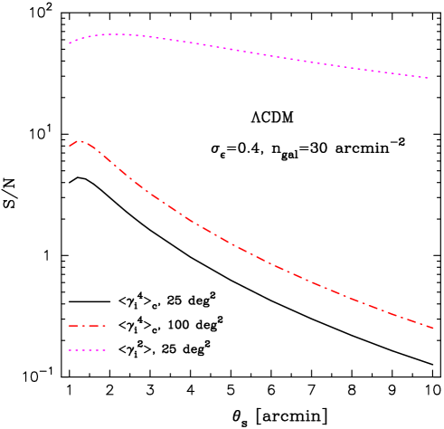
Figure 19: Estimates of the signal-to-noise ratio in the measurement of the connected fourth-order moment of the shear field, $\langle{\gamma_{i}^{4}}\rangle_{c}$, for the $\Lambda$CDM model against the smoothing scale. We assume $\sigma_{\epsilon}=0.4$ and $n_{\rm gal}=30~{}{\rm arcmin}^{-2}$ for the rms intrinsic ellipticity and the number density of source galaxies, and take the survey area to be $\Omega_{\rm survey}=25~{}{\rm degree}^{2}$. For comparison, the dotted and dot-dashed lines are the results for the shear variance and $\langle{\gamma_{i}^{4}}\rangle_{c}$ with $\Omega_{\rm survey}=100~{}{\rm degree}^{2}$, respectively.

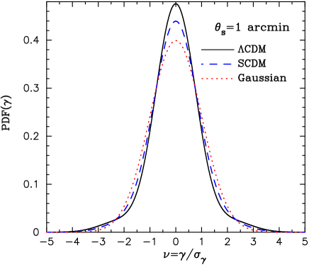
Figure 20: The probability distribution function (PDF) of the shear field. The solid and dashed lines are PDFs for the LCDM and SCDM models and $\theta_{\rm s}=1^{\prime}$, which are calculated using the Edgeworth expansion (44), while the dotted line is the Gaussian PDF.

For this purpose, it is crucial to correctly model possible errors in measurements of the shear, since higher-order statistics can be very sensitive to the noise. The main sources of error are the shot noise due to the intrinsic ellipticities of source galaxies and the sampling error for a finite survey area. If the intrinsic ellipticity distribution is regarded as Gaussian owing to random intrinsic orientations, we can estimate the dispersion for a measurement of the connected fourth-order moment of the shear field, $\langle{\gamma_{i}^{4}}\rangle_{c}$, following the method developed in §5 in Schneider et al. (1998):

$$\sigma(\langle{\gamma_{i}^{4}}\rangle_{c})\approx\frac{\theta_{\rm s}}{\sqrt{\Omega_{\rm survey}}}\sqrt{5451\times\sigma_{\gamma}^{8}(\theta_{\rm s})+\frac{24}{(\pi\theta_{\rm s}^{2}n_{\rm gal})^{4}}\left(\frac{\sigma_{\epsilon}^{2}}{2}\right)^{4}},$$ (43)

where $\sigma_{\epsilon}$ is the dispersion of the intrinsic ellipticity distribution, $\Omega_{\rm survey}$ the survey area and $n_{\rm gal}$ the number density of source galaxies. The first term on the r.h.s of the equation above denotes the sample variance and the second term the noise due to the finite number of randomly located source galaxy images. Here we have assumed $n_{\rm gal}\theta_{\rm s}^{2}\gg 1$ and that the connected part of the higher-order moments of the shear field is equal to its unconnected part for simplicity . Figure 19 shows an estimate of the signal-to-noise ratio in the measurement of $\langle{\gamma_{i}^{4}}\rangle_{c}$ for the $\Lambda$CDM model at $z_{\rm s}=1$, where we have assumed $n_{\rm gal}=30~{}{\rm arcmin}^{-2}$ and $\sigma_{\epsilon}=0.4$ and considered two cases of $\Omega_{\rm survey}=25$ and $100~{}{\rm deg}^{2}$. Note that a signal-to-noise ratio for the measurement of $S_{\gamma,4}$ is similar for the result in this figure, since the error arises mainly from the measurement of $\langle{\gamma_{i}^{4}}\rangle_{c}$ compared with that of $\langle{\gamma_{i}^{2}}\rangle$, as shown by comparing the solid and dotted lines. The noise is mainly due to the sample variance at $\theta_{\rm s}\lower 2.15277pt\hbox{$\;\buildrel>\over{\sim}\;$}2^{\prime}$ for the $\Lambda$CDM model, while the intrinsic ellipticity noise is important at $\theta_{\rm s}\lower 2.15277pt\hbox{$\;\buildrel<\over{\sim}\;$}2^{\prime}$. One can see that for a survey area of 25 square degrees the measurement of $\langle{\gamma_{i}^{4}}\rangle_{c}$ would indeed be marginally feasible on small angular scales $\theta_{\rm s}\lower 2.15277pt\hbox{$\;\buildrel<\over{\sim}\;$}3^{\prime}$, provided systematic errors can be kept under control. The results also imply an interesting possibility as discussed in Figure 15: a shallower survey, for a given amount of observing time, could improve the signal-to-noise ratio because the amplitude of $\langle{\gamma_{i}^{4}}\rangle_{c}$ does not decrease as much as that of the variance for low redshift structures. Further the redshift distribution is easier to measure accurately for a shallower survey. In any case, with a survey area exceeding 100 square degrees, expected from forthcoming lensing surveys, the kurtosis measurement should be made with high statistical significance, as shown by the dot-dashed line, and thus prove useful for parameter estimation.

There are some uncertainties we have ignored in the rough signal-to-noise estimate of equation (43). First, non-Gaussian errors are more important on smaller angular scales [Cooray & Hu 2001b], so sample variance must be estimated by using an adequate number of realizations of ray-tracing simulations or possibly by an analytical treatment using the halo approach for calculating the connected sixth- and eighth-order moments. Second, in actual data the noise distribution of the intrinsic ellipticities is likely to be non-Gaussian. In addition, we should bear in mind that the shear kurtosis is strongly affected by rare events in the tail of the measured shear distribution. Hence, we will need to consider some strategy to efficiently extract the shear kurtosis from realistic data which is less sensitive to unphysical rare events. One possible way to reduce the sample variance from such rare events is to use the probability distribution function (PDF) of the shear field, which is analogous to the method proposed by JSW for the study of the convergence skewness parameter. If the primordial fluctuations are Gaussian, the nonlinear gravitational evolution of structure formation induces the non-Gaussianity in the weak lensing fields, as investigated in this paper, and the weakly non-Gaussian PDF of the shear field can be modeled by the Edgeworth expansion (see Juszkiewicz et al. 1995). At the lowest order, we have

$$P(\gamma_{i})=\frac{1}{\sqrt{2\pi}\sigma_{\gamma}(\theta_{\rm s})}\exp\left(-\frac{\gamma_{i}^{2}}{2\sigma_{\gamma}^{2}(\theta_{\rm s})}\right)\left[1+\frac{1}{4{\rm!}}S_{\gamma,4}(\theta_{\rm s})\sigma_{\gamma}^{2}(\theta_{\rm s})H_{4}\left(\frac{\gamma_{i}}{\sigma_{\gamma}(\theta_{\rm s})}\right)\right],$$ (44)

where $H_{4}(x)=x^{4}-6x^{2}+3$ is the fourth-order Hermite polynomial. The resulting PDFs for the SCDM and $\Lambda$CDM models are shown in Figure 20. Moreover, in practice we must account for the fact that the measured shear field is a sum of the cosmic shear and noise fields. To obtain the PDF for the measured shear field $\gamma_{i}^{\rm obs}$, therefore, we have to convolve $P(\gamma_{i})$ with the PDF of the noise, where the noise field is defined by smoothing the intrinsic ellipticities of source galaxies contained within top-hat apertures. Note that there are two noise fields ($\epsilon_{1}$ and $\epsilon_{2}$) corresponding to the two shear fields ($\gamma_{1}$ and $\gamma_{2}$), respectively. If the noise PDF is given by $P_{N}(\epsilon_{i})$, the PDF for the measured shear field, $\gamma_{i}^{\rm obs}$, can be expressed by the convolution integral as

$$P(\gamma^{\rm obs}_{i}) = \int\!\!d\epsilon\int\!\!d\gamma_{i}P_{N}(\epsilon_{i})P(\gamma_{i})\delta_{D}(\gamma_{i}^{\rm obs}-\gamma_{i}-\epsilon),$$ (45)

where $P_{N}(\epsilon_{i})$ is normalized as $\int\!\!d\epsilon_{i}P_{N}(\epsilon_{i})=1$. It is worth noting that the noise PDF $P_{N}(\epsilon_{i})$ can also be modeled in terms of the variance and higher-order moments of the noise field using the Edgeworth expansion. Furthermore, this method can utilize a great advantage – the noise PDF $P_{N}(\epsilon_{i})$ can be directly reconstructed from the observed shear field, e.g. by smoothing after the randomization of the position angle of each galaxy image. This procedure would wash out the coherent cosmic shear pattern within the smoothing aperture, but pick up the contribution from the intrinsic ellipticities of source galaxies. In this sense, the variance and higher-order moments of the noise field for a given smoothing scale can be directly extracted from the measured data, giving an estimator for the noise PDF. To obtain the noise for the convergence field is harder, since a non-local reconstruction from the smoothed intrinsic ellipticity field is required [Van Waerbeke 1999]. For the shear, the theoretical model (45) for $P(\gamma^{\rm obs}_{i})$ is given by a single parameter, $S_{\gamma,4}(\theta_{\rm s})$. One can then fit the theoretical prediction to the measured PDF over an appropriate intermediate range of $\gamma^{\rm obs}_{i}$, where the Edgeworth expansion is valid, to extract the shear kurtosis $S_{\gamma,4}$ with reduced sensitivity to rare events. The quantitative improvement in the signal-to-noise will be the subject of a later study.

Other uncertainties we have ignored in this paper are effects of the redshift distribution of source galaxies and the clustering of source galaxies. Figure 15 shows that the higher-order moments are more sensitive to nonlinear structures at lower redshifts than the variance and, as a result, the shear kurtosis can be sensitive to the source redshift distribution. Consider the conventionally used model for the redshift distribution of source galaxies

$$n(z)=\frac{\beta}{z_{0}\Gamma(\frac{1+\alpha}{\beta})}\left(\frac{z}{z_{0}}\right)^{\alpha}\exp\left[-\left(\frac{z}{z_{0}}\right)^{\beta}\right],$$ (46)

with $\alpha=2$ and $\beta=1.2$ (e.g., see van Waerbeke et al. (2002)) and the source redshift parameter $z_{0}=0.48$, so that it gives the mean source redshift $\langle{z_{s}}\rangle\approx 1.0$. This distribution increases the value of $S_{\gamma,4}$ at $\theta_{\rm s}=1^{\prime}$ by $\sim 20\%$ for the SCDM and $\Lambda$CDM models, compared to the case with source redshifts fixed at $z_{s}=1$. This increase is to some extent counterbalanced by the source clustering effect, because previous work based on perturbation theory [Bernardeau 1998] showed that source clustering reduces the values of the convergence skewness and kurtosis by $\sim 10-20\%$ (recently confirmed by ray-tracing simulation [Hamana et al. 2002] as well as by an analytical study [Schneider, Van Waerbeke & Mellier 2001]). It is reasonable to expect that this argument is also valid for the shear kurtosis, because we showed $S_{\gamma,4}$ is related to the convergence kurtosis $S_{\kappa,4}$ through a geometrical constant factor (see discussions around equation (42)).

Although the halo approach used here and in the literature assumes a spherically symmetric profile, in reality halos have non-spherical profiles and substructure as predicted in the CDM paradigm (e.g., Jing & Suto 2001). Our results showed that the halo model can fairly reproduce the ray-tracing simulation results for the 1-point moments of the smoothed lensing fields. This success is encouraging, since the simulations include contributions from various realistic halo profiles. The agreement is partly because we focus only on statistical quantities and, therefore, to some extent the profile we need for the halo model calculation should be an average over possible halo profiles of a given mass. In addition, 1-point moments of the smoothed fields are likely to be insensitive to halo profile fluctuations. We expect that the full 3- or 4-point correlation functions of the lensing fields would be more sensitive to profile fluctuations, because those functions should contain complete information on gravitational clustering up to the 3 or 4-point level through the configuration dependences. These issues will be presented elsewhere (Takada & Jain 2002).

Finally, we comment on an alternative application of measurements of the shear kurtosis. If cosmological parameters including $\Omega_{\rm m0}$ are precisely determined by other measurements, our results suggest that the higher-order moments of weak lensing fields could be used to constrain dark matter halo profiles. This problem is particularly interesting, since it can be a clue to understanding the nature of dark matter. Although the concentration and inner profile of dark matter halo are degenerate in giving two-point lensing statistics as argued in this paper (see also Seljak 2000), a detailed study may yield ways of combining the two-point and four-point shear statistics to break the degeneracy by exploiting the dependences of the shear kurtosis on the inner profile and the concentration parameter shown in Figure 16. If this is the case, Figure 13 indicates that measurements of the shear kurtosis at $\theta_{\rm s}\lower 2.15277pt\hbox{$\;\buildrel>\over{\sim}\;$}1^{\prime}$ can constrain the properties of the halo profile at mass scales $M\lower 2.15277pt\hbox{$\;\buildrel>\over{\sim}\;$}10^{14}M_{\odot}$.

We would like to thank T. Hamana for kindly providing his ray-tracing simulation data as well as for fruitful comments. This work benefitted from several discussions with R. Scoccimarro. We also thank E. Komatsu, A. Taruya and L. van Waerbeke for valuable discussions and D. Dolney for a careful reading of the manuscript. This work is supported in part by the Japan Society for Promotion of Science (JSPS) Research Fellowships, a NASA-LTSA grant, and a Keck foundation grant.

Appendix A Perturbation theory bispectrum and trispectrum

The explicit forms of the bispectrum and trispectrum of the density field based on perturbation theory (e.g., Fry 1984) are

$$B^{\rm pt}(\mbox{{\it\boldmath$k$}}_{1},\mbox{{\it\boldmath$k$}}_{2},\mbox{{\it\boldmath$k$}}_{3},z) = 2F_{2}(\mbox{{\it\boldmath$k$}}_{1},\mbox{{\it\boldmath$k$}}_{2})P^{L}(k_{1},z)P^{L}(k_{2},z)+\mbox{2 perm.},$$ (47)

$$T^{\rm pt}(\mbox{{\it\boldmath$k$}}_{1},\mbox{{\it\boldmath$k$}}_{2},\mbox{{\it\boldmath$k$}}_{3},\mbox{{\it\boldmath$k$}}_{4};z) = 4\left[F_{2}(\mbox{{\it\boldmath$k$}}_{13},-\mbox{{\it\boldmath$k$}}_{1})F_{2}(\mbox{{\it\boldmath$k$}}_{13},\mbox{{\it\boldmath$k$}}_{2})P^{L}(k_{13},z)P^{L}(k_{1},z)P^{L}(k_{2},z)+\mbox{11 perm.}\right]$$ (48)

$$+6\left[F_{3}(\mbox{{\it\boldmath$k$}}_{1},\mbox{{\it\boldmath$k$}}_{2},\mbox{{\it\boldmath$k$}}_{3})+P^{L}(k_{1},z)P^{L}(k_{2},z)P^{L}(k_{3},z)+\mbox{3 term}\right],$$

where the redshift evolution of the linear power spectrum is given by $P^{L}(k,z)=D^{2}(z)P^{L}(k,z=0)$ where $D(z)$ is the growth factor. The kernels $F_{n}$ are calculated using perturbation theory (e.g., see Jain & Bertschniger 1994) and are expressed as

$$F_{2}(\mbox{{\it\boldmath$k$}}_{1},\mbox{{\it\boldmath$k$}}_{2}) = \frac{5}{7}+\frac{1}{2}\left(\frac{1}{k_{1}^{2}}+\frac{1}{k_{2}^{2}}\right)(\mbox{{\it\boldmath$k$}}_{1}\cdot\mbox{{\it\boldmath$k$}}_{2})+\frac{2}{7}\frac{(\mbox{{\it\boldmath$k$}}_{1}\cdot\mbox{{\it\boldmath$k$}}_{2})^{2}}{k_{1}^{2}k_{2}^{2}},$$

$$F_{3}(\mbox{{\it\boldmath$k$}}_{1},\mbox{{\it\boldmath$k$}}_{2},\mbox{{\it\boldmath$k$}}_{3}) = \frac{7}{18}\frac{\mbox{{\it\boldmath$k$}}_{12}\cdot\mbox{{\it\boldmath$k$}}_{1}}{k_{1}^{2}}\left[F_{2}(\mbox{{\it\boldmath$k$}}_{2},\mbox{{\it\boldmath$k$}}_{3})+G_{2}(\mbox{{\it\boldmath$k$}}_{1},\mbox{{\it\boldmath$k$}}_{2})\right]+\frac{1}{18}\frac{k_{12}^{2}(\mbox{{\it\boldmath$k$}}_{1}\cdot\mbox{{\it\boldmath$k$}}_{2})}{k_{1}^{2}k_{2}^{2}}\left[G_{2}(\mbox{{\it\boldmath$k$}}_{2},\mbox{{\it\boldmath$k$}}_{3})+G_{2}(\mbox{{\it\boldmath$k$}}_{1},\mbox{{\it\boldmath$k$}}_{2})\right],$$ (49)

with

$$G_{2}(\mbox{{\it\boldmath$k$}}_{1},\mbox{{\it\boldmath$k$}}_{2})=\frac{3}{7}+\frac{1}{2}\left(\frac{1}{k_{2}^{2}}+\frac{1}{k^{2}_{1}}\right)\frac{\mbox{{\it\boldmath$k$}}_{1}\cdot\mbox{{\it\boldmath$k$}}_{2}}{k_{1}k_{2}}+\frac{4}{7}\left(\frac{\mbox{{\it\boldmath$k$}}_{1}\cdot\mbox{{\it\boldmath$k$}}_{2}}{k_{1}k_{2}}\right)^{2},$$ (50)

where we have ignored the extremely weak dependences of the functions $F_{n}$ and $G_{2}$ on cosmological parameters $\Omega_{\rm m0}$ and $\Omega_{\lambda 0}$.

Appendix B Geometrical properties of top-hat filter function

The purpose of this Appendix is to derive properties of the integrals of products of the two-dimensional top-hat kernel given by equation (23). This is analogous to the approach in Appendix B of Bernardeau (1994).

We begin our discussion with deriving the following identity for the third-order products, since it is relevant for the calculation of the third-order moment of weak lensing fields (see §4):

$$\int\!\!\frac{d^{2}\mbox{{\it\boldmath$x$}}_{1}}{(2\pi)^{2}}\int\!\!\frac{d^{2}\mbox{{\it\boldmath$x$}}_{2}}{(2\pi)^{2}}F(x_{1})F(x_{2})F(x_{12})=\int_{0}^{\infty}\!\!\frac{x_{1}dx_{1}}{2\pi}\int_{0}^{\infty}\!\!\frac{x_{2}dx_{2}}{2\pi}F^{2}(x_{1})F^{2}(x_{2}),$$ (51)

where the top-hat kernel is $F(x)=2J_{1}(x)/x$ and $x_{12}\equiv|\mbox{{\it\boldmath$x$}}_{1}+\mbox{{\it\boldmath$x$}}_{2}|$.

The proof of equation (51) is as follows. From the expansion formula of Bessel function (e.g., 8.532.1 in Gradshteyn & Ryzhik 2000) we can expand the kernel $F(|\mbox{{\it\boldmath$x$}}_{1}+\mbox{{\it\boldmath$x$}}_{2}|)$ as

$$F(|\mbox{{\it\boldmath$x$}}_{1}+\mbox{{\it\boldmath$x$}}_{2}|)=2\frac{J_{1}(|\mbox{{\it\boldmath$x$}}_{1}+\mbox{{\it\boldmath$x$}}_{2}|)}{|\mbox{{\it\boldmath$x$}}_{1}+\mbox{{\it\boldmath$x$}}_{2}|} = 4\sum_{n=0}(n+1)\frac{J_{n+1}(x_{1})}{x_{1}}\frac{J_{n+1}(x_{2})}{x_{2}}(-1)^{n}\frac{\sin[(n+1)\Phi_{2}]}{\sin\Phi_{2}},$$ (52)

where $\Phi_{2}$ is the angle between $\mbox{{\it\boldmath$x$}}_{1}$ and $\mbox{{\it\boldmath$x$}}_{2}$, giving $x_{12}=(x_{1}^{2}+x_{2}^{2}-2x_{1}x_{2}\cos\Phi_{2})^{1/2}$. Inserting this equation into the left part of equation (51) and then integrating it over the angle $\Phi_{2}$, we obtain

$$\int\!\!\frac{x_{1}dx_{1}}{2\pi}\frac{x_{2}dx_{2}}{2\pi}F(x_{1})F(x_{2})\left[F(x_{1})F(x_{2})-12\frac{J_{3}(x_{1})}{x_{1}}\frac{J_{2}(x_{2})}{x_{2}}+20\frac{J_{5}(x_{1})}{x_{1}}\frac{J_{5}(x_{2})}{x_{2}}+\cdots\right],$$ (53)

Using the recursion relation for Bessel functions and an integration formula (6.574.2 in Gradshteyn & Ryzhik 2000), the second term in the bracket on the r.h.s of equation above vanishes because

$$\int^{\infty}_{0}\!\!\frac{x_{1}dx_{1}}{2\pi}\frac{J_{1}(x_{1})}{x_{1}}\frac{J_{3}(x_{1})}{x_{1}} = \int^{\infty}_{0}\!\!\frac{x_{1}dx_{1}}{2\pi}\frac{J_{1}(x_{1})}{x_{1}}\left[4\frac{J_{2}(x_{1})}{x_{1}^{2}}-\frac{J_{1}(x_{1})}{x_{1}}\right]$$ (54)

$$= 4\cdot 2^{-1}\frac{\Gamma(2)\Gamma(1)}{\Gamma(3/2)\Gamma(5/2)\Gamma(1/2)}-\frac{\Gamma(1)\Gamma(1/2)}{\Gamma(1/2)\Gamma(3/2)\Gamma(1/2)}$$

$$= \frac{1}{2}-\frac{1}{2}=0.$$

One can similarly find that the third term and higher terms in the bracket on the r.h.s of equation (53) vanish, and then equation (51) follows.

Likewise, one can straightforwardly obtain the following identity on which the approximation for calculating the convergence forth-order moment is based:

$$\int\!\!\prod_{i=1}^{3}\frac{d^{2}\mbox{{\it\boldmath$x$}}_{i}}{(2\pi)^{2}}F(x_{1})F(x_{2})F(x_{3})F(x_{123})=\int\!\!\prod_{i=1}^{3}\frac{x_{i}dx_{i}}{2\pi}F^{2}(x_{1})F^{2}(x_{2})F^{2}(x_{3}),$$ (55)

where $x_{123}\equiv|\mbox{{\it\boldmath$x$}}_{1}+\mbox{{\it\boldmath$x$}}_{2}+\mbox{{\it\boldmath$x$}}_{3}|$.

Appendix C 2-halo and 3-halo contributions to the convergence fourth-order moment

In this Appendix, we write down the expressions for approximations used for calculations of the 2-halo and 3-halo contributions to the convergence fourth-order moment, which are discussed in §4.

The 2-halo term of the convergence fourth-order moment receives two contributions, which represent taking three or two particles in the first halo:

$$\langle{\kappa^{4}}\rangle^{2h}_{c}=\int\!\!d\chi W^{4}(\chi,\chi_{\rm s})d_{A}^{-4}(\chi)\int\!\!\!\prod_{i=1}^{3}\frac{d^{2}\mbox{{\it\boldmath$l$}}_{i}}{(2\pi)^{2}}\left[T^{2h}_{31}+T^{2h}_{22}\right](\mbox{{\it\boldmath$l$}}_{1},\mbox{{\it\boldmath$l$}}_{2},\mbox{{\it\boldmath$l$}}_{3},-\mbox{{\it\boldmath$l$}}_{123})F(l_{i})F(l_{123}),$$ (56)

where $T^{2h}_{31}$ and $T^{2h}_{22}$ are given by equations (15) and (16), and $\mbox{{\it\boldmath$k$}}_{i}=\mbox{{\it\boldmath$l$}}_{i}/d_{A}(\chi)$. It is clear that the contribution from $T^{2h}_{31}$ dominates that from $T^{2h}_{22}$, because the former arises mainly from 3-point correlations within one halo with a highly nonlinear density contrast, while the latter arises from 2-point correlations. We confirmed that the $T^{2h}_{22}$ contribution is smaller even than the 3-halo term. For this reason, we ignore the $T^{2h}_{22}$ contribution and use the following approximation for calculating the 2-halo term in the convergence fourth-order moment (we also include the approximation for $F(l_{123})$ from equation (33)):

$$\langle{\kappa^{4}}\rangle^{2h}_{c} \approx 4\int\!\!d\chi W^{4}(\chi,\chi_{\rm s})d_{A}^{-6}(\chi)\int\!\!dM_{1}\frac{dn}{dM_{1}}\left(\frac{M_{1}}{\bar{\rho}_{0}}\right)^{3}b(M_{1},z)\int\!\!\frac{l_{1}dl_{1}}{2\pi}\frac{l_{2}dl_{2}}{2\pi}y(l_{1},M_{1})y(l_{2},M_{1})y(\tilde{l}_{12},M_{1})F^{2}(l_{1})F^{2}(l_{2})$$ (57)

$$\times\int\!\!dM_{2}\frac{dn}{dM_{2}}b(M_{2},z)\left(\frac{M_{2}}{\bar{\rho}_{0}}\right)\int\!\!\frac{l_{3}dl_{3}}{2\pi}y(l_{3},M_{3})F^{2}(l_{3})P^{L}(l_{3}),$$

where $\tilde{l}_{12}=(l_{1}^{2}+l_{2}^{2}-l_{1}l_{2})^{1/2}$ and the factor of $4$ comes from the permutation symmetry in the 2-halo trispectrum (see equation (15)) for the fourth-order moment calculation. We have written the order of integration specifically to point out that the last two integrals, over $M_{2}$ and $l_{3}$, can be performed separately from the preceding three. Thus one needs to perform at most a 4-dimensional numerical integration to get $\langle{\kappa^{4}}\rangle^{2h}_{c}$.

Similarly, we use the following equation to calculate the 3-halo term in the convergence fourth-order moment:

$$\langle{\kappa^{4}}\rangle^{3h}_{c} \approx 6\int\!\!d\chi W^{4}(\chi,\chi_{\rm s})d_{A}^{-6}(\chi)\int\!\!\frac{l_{1}dl_{1}}{2\pi}\frac{d^{2}\mbox{{\it\boldmath$l$}}_{2}}{(2\pi)^{2}}B^{\rm pt}(\mbox{{\it\boldmath$l$}}_{1},\mbox{{\it\boldmath$l$}}_{2},-\mbox{{\it\boldmath$l$}}_{12})F^{2}(l_{1})F^{2}(l_{2})\int\!\!dM_{1}\frac{dn}{dM_{1}}\frac{M_{1}}{\bar{\rho}_{0}}b(M_{1},z)y(l_{1},M_{1})$$ (58)

$$\times\int\!\!dM_{2}\frac{dn}{dM_{2}}\frac{M_{2}}{\bar{\rho}_{0}}b(M_{2},z)y(l_{2},M_{2})\int\!\!dM_{3}\frac{dn}{dM_{3}}\left(\frac{M_{3}}{\bar{\rho}_{0}}\right)^{2}b(M_{3},z)\int\!\!\frac{l_{3}dl_{3}}{2\pi}y^{2}(l_{3},M_{3})F^{2}(l_{3}),$$

where $d^{2}\mbox{{\it\boldmath$l$}}_{2}=l_{2}ddl_{2}d\Phi_{2}$, $l_{12}=(l_{1}+l_{2}-2l_{1}l_{2}\cos\Phi_{2})^{1/2}$ and the factor of 6 comes from equation (17). We have used the approximation $y(l_{123})=y(l_{3})$, which is valid to high accuracy for the 3-halo term. Again, a careful consideration of the dependences of the integrated functions reveals that we have to perform only a 4-dimensional numerical integration to obtain $\langle{\kappa^{4}}\rangle^{3h}_{c}$.

References

- [Bacon, Refregier & Ellis 2000] Bacon, D., Refregier, A., Ellis, R., 2000, MNRAS, 318, 625
- [Bacon et al. 2002] Bacon, D., Massey, R., Refregier, A., Ellis, R., 2002, astro-ph/0203134
- [Bardeen et al. 1986] Bardeen, J. M., Bond, J. R., Kaiser, N., Szalay, A. S., 1986, ApJ, 304, 15
- [Bartelmann & Schneider 2001] Bartelmann, M., Schneider, P., 2001, Phys. Rep. 340, 291
- [Bernardeau 1994] Bernardeau, F., 1994, ApJ, 427, 51
- [Bernardeau 1998] Bernardeau, F., 1998, A&A, 338, 375
- [Bernardeau, Mellier & Van Waerbeke 2002b] Bernardeau, F., Mellier, Y., Van Waerbeke, L., 2002b, astro-ph/0201032
- [Bernardeau, Van Waerbeke & Mellier 1997] Bernardeau, F., Van Waerbeke, L., Mellier, Y., 1997, A&A, 322, 1
- [Bernardeau, Van Waerbeke & Mellier 2002a] Bernardeau, F., Van Waerbeke, L., Mellier, Y., 2002a, astro-ph/0201029 (BvWM)
- [Blandford et al. 1991] Blandford, R. D., Saust, A. B., Brainerd, T. G., Villumsen, J. V., 1991, MNRAS, 251, 600
- [Bullock et al. 2001] Bullock, J. S., Kolatt, T. S., Sigad, Y., Somerville, R. S., Kravtsov, A. V., Klypin, A. A., Primack, J. R., Dekel, A., 2001, MNRAS, 321, 559
- [Cooray & Hu 2001a] Cooray, A., Hu, W., 2001a, ApJ, 548, 7
- [Cooray & Hu 2001b] Cooray, A., Hu, W., 2001b, ApJ, 554, 56
- [Cooray & Sheth 2002] Cooray, A., Sheth, R., 2002, to appear in Physics Reports
- [Cooray et al. 2000] Cooray, A., Hu, W., Miralda-Escude, J., 2000, ApJ, 535, L9
- [Gradshteyn & Ryzhik 2000] Gradshteyn, L. S., Ryzhik, I. M., 2000, Tabel of Integrals, Series, and Products, (6th ed.; San Diego, Academic Press)
- [Guzik & Seljak 2002] Guzik, J., Seljak, U., 2002, astro-ph/0201448
- [Eke, Cole & Frenk 1996] Eke, V. R., Cole, S., Frenk, C. S., 1996, MNRAS, 282, 263
- [Fry 1984] Fry, J. N., 1984, ApJ, 279, 499
- [Fukushige & Makino 1997] Fukushige, T., Makino, J., 1997, ApJ, 477, L9
- [Fukushige & Makino 2001] Fukushige, T., Makino, J., 2001, ApJ, 557, 533
- [Haemmerle et al. 2002] Haemmerle, H., J.-M. Miralles, J.-M., Schneider, P., Erben, T., Fosbury, R. A. E., Freudling, W., Pirzkal, N., Jain, B., S. D. M. White, S. D. M., 2002, A&A, 385, 743
- [Hamana 2002] Hamana, T., 2002, private communication
- [Hamana & Mellier 2001] Hamana, T., Mellier, Y., 2001, MNRAS, 327, 169 (HM)
- [Hamana et al. 2002] Hamana, T., Colombi, S. T., Thion, A., Devriendt, J. E. G. T., Mellier, Y., Bernardeau, F., 2002, MNRAS, 330, 365
- [Henry 2000] Henry, J. P., 2000, apj, 534, 565
- [Hoekstra et al. 2002] Hoekstra, H., Yee, H. K. C., Gladders, M. D., Barrientos, L. F., Hall, P. B., Infante, L., 2002, ApJin press, astro-ph/0202285
- [Hui 1999] Hui, L., 1999, ApJ, 519, L9
- [Jain & Bertschinger 1994] Jain, B., Bertschinger, E., 1994, ApJ, 431, 495
- [Jain & Seljak 1997] Jain, B., Seljak, U., 1997, ApJ, 484, 560
- [Jain, Seljak & White 2000] Jain, B., Seljak, U., White, S. D. M., 2000, ApJ, 530, 547 (JSW)
- [Jenkins et al. 1998] Jenkins, A., et al., 1998, ApJ, 499, 20
- [Jimenez, Verde & Oh 2002] Jimenez, R., Verde, L., Oh, S. P., 2002, astro-ph/0201352
- [Jing 2000] Jing, Y. P., 2000, ApJ, 535, 30
- [Jing & Suto 2000] Jing, Y. P., Suto, Y., 2000, ApJ, 529, L69
- [Jing & Suto 2002] Jing, Y. P., Suto, Y., 2002, ApJ, 574, 538
- [Juszkiewicz et al. 1995] Juszkiewicz, R., Weinberg, D. H., Amsterdamski, P., Chodorowski, M., & Bouchet, F. 1995, ApJ, 442, 39
- [Kaiser 1992] Kaiser, N., 1992, ApJ, 388, 272
- [Kaiser 1998] Kaiser, N., 1998, ApJ, 498, 26
- [Kaiser et al. 1994] Kaiser, N., Squires, G., Fahlman, G., Woods, D., 1994, in Durret, F., Mazure, A., Tran Thanh Van, J., Eds., Clusters of Galaxies. Editions Frontières. Gif-sur-Yvette, p. 269
- [Kaiser, Wilson & Luppino 2000] Kaiser, N., Wilson, G., Luppino, G. A., 2000, astro-ph/0003338
- [Komatsu & Kitayama 1999] Komatsu, E., Kitayama, T., 1999, ApJ, 526, L1
- [Lahav et al. 2001] Lahav, O., et al. 2001, astro-ph/0112162
- [Limber 1954] Limber, D., 1954, ApJ, 119, 655
- [Ma & Fry 2000] Ma, C.-P. Fry, J. N., 2000, ApJ, 543, 503
- [Maoli et al. 2001] Maoli, R., Van Waerbeke, L., Mellier, Y., Schneider, P., Jain, B., Bernardeau, F., Erbe, T., Fort, B., 2001, A&A 368, 766
- [Matsubara & Jain 2001] Matsubara, T., Jain, B., 2001, ApJ, 552, L89
- [McClelland & Silk 1977] McClelland, J., Silk, J., 1977, ApJ, 217, 331
- [Mellier 1999] Mellier, Y., 1999, ARAA, 37, 127
- [Miralda-Escude 1991] Miralda-Escude, J., 1991, ApJ, 380, 1
- [Mo & White 1996] Mo, H. J., White, S. D. M., 1996, MNRAS, 282, 347
- [Mo, Jing & White 1997] Mo, H. J., Jing, Y. P., White, S. D. M., 1997, MNRAS, 290, 651
- [Moore et al. 1998] Moore, B., Governato, F., Quinn, T., Stadel, J., Lake G., 1998, ApJ, 499, L5
- [Munshi & Jain 2001] Munshi, D., Jain, B., 2001, MNRAS, 322, 107
- [Nakamura & Suto 1997] Nakamura, T. T., Suto, Y., 1997, Prog. Theor. Phys., 97, 49
- [Navarro, Frenk & White 1996] Navarro, J., Frenk, C., White, S. D. M., 1996, ApJ, 462, 564 (NFW)
- [Navarro, Frenk & White 1997] Navarro, J., Frenk, C., White, S. D. M., 1997, ApJ, 490, 493 (NFW)
- [Netterfield et al. 2001] Netterfield, C. B., et al., 2001, ApJ in press, astro-ph/0104460
- [Peacock & Doods 1996] Peacock, J. A., Dodds, S. J., 1996, MNRAS, 280, L19
- [Peebles 1980] Peebles, P. J. E., 1980, Large-Scale Structure of the Universe (Princeton: Princeton Univ. Press)
- [Press & Schechter 1974] Press, W., Schechter, P., 1974, ApJ, 187, 425
- [Refregier, Rhodes & Groth 2002] Refregier, A., Rhodes, J., Groth, E., 2002, astro-ph/0203131
- [Rhodes, Refregier & Groth 2001] Rhodes, J., Refregier, A., Groth, E., 2001, ApJ, 552, L85
- [Sato et al. 2001] Sato, J., Takada, M., Jing, Y. P., Futamase, T., 2001, ApJ, 551, L5
- [Scherrer & Bertschinger 1991] Scherrer, R. J., Bertschinger, E., 1991, ApJ, 381, 349
- [Schneider 1996] Schneider, P., 1996, MNRAS, 283, 837
- [Schneider, Van Waerbeke & Mellier 2001] Schneider, P., Van Waerbeke, L., Mellier, Y., 2001, astro-ph/0112441
- [Schneider et al. 1998] Schneider, P., Van Waerbeke, L., Jain, B., Kruse, G., 1998, MNRAS, 296, 873
- [Scoccimarro & Friemann 1999] Scoccimarro, R., Friemann, J., 1999, MNRAS, 520, 35
- [Scoccimarro et al. 2001] Scoccimarro, R., Sheth, R. K., Hui, L., Jain, B., 2001, ApJ, 546, 652
- [Seljak 2000] Seljak, U., 2000, MNRAS, 318, 203
- [Seljak 2001] Seljak, U., 2001, astro-ph/0111362
- [Seljak 2002] Seljak, U., 2002, astro-ph/0201450
- [Sheth & Lemson 1999] Sheth, R. K., Jain, B., 1997, MNRAS, 285, 231
- [Sheth & Lemson 1999] Sheth, R. K., Lemson, G., 1999, MNRAS, 304, 767
- [Sheth & Tormen 1999] Sheth, R. K., Tormen, G., 1999, MNRAS, 308, 119
- [Takada & Jain 2002] Takada, M., Jain, B., 2002, in preparation
- [Takada, Jain & Hamana 2002] Takada, M., Jain, B., Hamana, T., 2002, in preparation
- [Taruya et al. 2002] Taruya, A., Takada, M., Hamana, T., Kayo, I., Futamase, T., 2002, ApJ in press, astro-ph/0202090
- [Van Waerbeke 1999] Van Waerbeke, L., 1999, MNRAS, 313, 524
- [Van Waerbeke et al. 2000] Van Waerbeke, L. et al., 2000, A&A, 358, 30
- [Van Waerbeke et al. 2001a] Van Waerbeke, L. et al., 2001a, A&A, 374, 757
- [Van Waerbeke, Bernardeau, Mellier 1999] Van Waerbeke, L., Bernardeau, F., Mellier, Y., 1999, A&A, 342, 15
- [Van Waerbeke et al. 2001b] Van Waerbeke, L., Hamana, T., Scoccimarro, R., Colombi, S., Bernardeau, F., 2001b, MNRAS, 322, 918
- [Van Waerbeke et al. 2002] Van Waerbeke, L., Mellier, Y., Pelló, R., Pen, U-L., McCracken, H. J., Jain, B., 2002, astro-ph/0202503
- [Villumsen 1996] Villumsen, J. V., 1996, MNRAS, 281, 369
- [White & Hu 2000] White, M., Hu, W., 2000, ApJ, 537, 1 (WH)
- [Wittman et al. 2000] Wittman, D.M., Tyson, J.A., Kirkman, D., Dell’Antonio, I., Bernstein, G., 2000, Nature, 405, 143