EFI-00-14

astro-ph/0205046

A PROTOTYPE SYSTEM FOR DETECTING THE RADIO-FREQUENCY

PULSE ASSOCIATED WITH COSMIC RAY AIR SHOWERS

Kevin Green, Jonathan L. Rosner, and Denis A. Suprun

Enrico Fermi Institute and Department of Physics

University of Chicago, Chicago, IL 60637

J. F. Wilkerson

Center for Experimental Nuclear Physics and Astrophysics

Department of Physics, University of Washington, Seattle, WA 98195

ABSTRACT

The development of a system to detect the radio-frequency (RF) pulse associated with extensive air showers of cosmic rays is described. This work was performed at the CASA/MIA array in Utah, with the intention of designing equipment that can be used in conjunction with the Auger Giant Array. A small subset of data (less than 40 out of a total of 600 hours of running time), taken under low-noise conditions, permitted upper limits to be placed on the rate and strength of pulses accompanying showers with energies around $10^{17}$ eV.

1 Motivation

As a result of work in the 1960’s and 1970’s [1, 2, 3, 4], some of which continued beyond then (see, e.g., [5, 6, 7, 8]), it appears that air showers of energy 10¹⁷ eV are accompanied by radio-frequency (RF) pulses [9], whose properties suggest that they are due mainly to the separation of positive and negative charges of the shower in the Earth’s magnetic field [10, 11]. The most convincing data were accumulated in the 30–100 MHz frequency range. However, opinions differ regarding the strength of the pulses, and atmospheric and ionospheric effects have led to irreproducibility of results. In particular, there may also be pulses associated with cosmic-ray-induced atmospheric discharges [12, 13]. There are reports of detection at MHz or sub-MHz frequencies [5, 6, 7], which could be associated with such a mechanism. Signals above 100 MHz have also been reported [8].

A study was undertaken of the feasibility of equipping the Auger array [14] with the ability to detect such pulses. The higher energy of the showers to which the array would be sensitive could change the parameters of detection. Before a design for large-scale RF pulse detection could be produced, it was necessary to retrace some of the steps of the past 30 years by searching for the pulses accompanying 10¹⁷ eV showers, and by studying some of the factors which led to their irreproducibility in the past. RF pulses may be able to provide auxiliary information about primary composition and shower height [3].

In this article we describe the prototype activity at the CASA/MIA site and draw some conclusions from it regarding plans for the Auger project. We have not been able to demonstrate the presence of RF pulses at CASA/MIA, and could only set upper limits for their intensity. The upper limits on the rates of events in which the North-South (or East-West) projection of the signal pulse was greater than some value were established at $R^{up}({\cal E}_{\nu NS}>{\cal E}_{\nu}^{0})=0.555/({\cal E}_{\nu}^{0})^{2}\$ h^-1 and $R^{up}({\cal E}_{\nu EW}>{\cal E}_{\nu}^{0})=0.889/({\cal E}_{\nu}^{0})^{2}\$ h^-1, respectively, with ${\cal E}_{\nu}$ being the electric field strength per unit of frequency, measured in $\mu{\rm V}/{\rm m}/{\rm MHz}$. More concrete plans for RF detection at Auger must await a prototype at the Auger site which utilizes some of the lessons learned from the present work. A preliminary description of this work was presented in Ref. [15].

In Sections 2 and 3 we discuss expectations for RF signals and previous claims of their observation. Section 4 is devoted to details of the setup at CASA/MIA, including some of the reasons for choosing the specific configuration utilized. Our preliminary results are given in Section 5, while Section 6 deals with issues specific to a giant array such as Auger. We summarize in Section 7. Appendix A gives details of the sensitivity calculation, Appendix B establishes some properties of simulated pulses, while Appendix C summarizes cost estimates for an installation at the Auger site.

2 Expectations

We briefly summarize some expectations [3] for the characteristic of the RF signal associated with cosmic ray air showers.

2.1 Mechanisms of pulse generation

In the 1950’s, R. R. Wilson [12] proposed that cosmic rays could induce the atmosphere to act as a giant spark chamber, triggering discharges of the ambient field gradient. This gradient, normally around 100 V/m, can attain values as high as 10 kV/m during intense thunderstorm activity [3]. Thus, the mechanism would lead to pulses of greatly varying intensity, whose correlation with air showers would be difficult to establish unless field gradients could be monitored over the whole path of the discharge.

Another mechanism of pulse generation is associated with the asymmetry in electron and positron yields in showers as a result of Compton and knock-on processes. By the end of the shower, electrons outnumber positrons by about 10–25%, leading to a transient of vertically moving negative charge [9]. This is thought to be the main mechanism for generation of radio-frequency signals from showers in solid material such as polar ice [16] or sand [17], but is probably not the dominant mechanism in the atmosphere.

Still another source of electromagnetic radiation in a cosmic ray shower involves the separation of positive and negative electric charges in the Earth’s magnetic field. This is thought to be the dominant mechanism accounting for atmospheric pulses with frequencies in the 30 – 100 MHz range, and will be taken as the model for the signal for which the search was undertaken.

2.2 Characteristic pulse

The time profile of a pulse due to charge-separation in the Earth’s magnetic field can be modelled [3] by assuming that the bulk of the shower giving rise to the pulse is concentrated between an altitude of 10 and 5 km (for a shower of energy $10^{17}$ eV) and calculating the pulse duration by comparing the total path lengths between the antenna and the beginning and the end of the shower. The rise time of a pulse from a shower with zero zenith angle observed 200 meters from its axis is expected to be about 5 ns, followed by a longer decay time and a still longer recovery time with opposite amplitude (about 100 ns) such that the total DC component is zero.

The radiation from any stage of the shower which is traveling directly toward the antenna is expected to arrive to the antenna about the same time as the shower itself. The difference is accounted for by the refraction index of air. Such an essentially $\delta$-function pulse has the highest-frequency components in its spectrum. Showers for which the impact parameters of the cores are farther from the antenna will have reduced high-frequency components since the total pulse duration will be longer, approaching several microseconds for vertically incident showers viewed from the side.

The pulse is expected to grow linearly in amplitude with shower energy as a result of the increased number of particles emitting RF energy. This linear growth assumes coherence of the emitting particles, which is probably a good assumption for RF wavelengths of several meters. The greater penetration of the atmosphere by more energetic showers also leads to an increased RF signal since the radiating particles are closer to the receiver. This should make the pulse amplitude increase more rapidly than linearly with primary energy. However, this effect is largely offset by the fact that a greater fraction of such deeply penetrating showers will have reduced high-frequency components in their pulses, as a result of the greater apparent time taken by the pulse to build up to its maximum amplitude at the receiver. The combination of the above three effects is expected to lead fortuitously to an overall linear dependence of pulse amplitude on primary energy [3].

At extremely high energies, shower particles will even be lost by collision with the Earth. This may give rise to a different type of RF signal but will not be effective in the context of the charge-separation mechanism considered here. The pulses associated with charge separation in the Earth’s magnetic field should correspond to radio signals with approximately horizontal polarization. (For showers not arriving vertically from directly overhead there will also be a small vertical polarization component.)

2.3 RF backgrounds

Discharges of atmospheric electricity constitute an important source of background pulses. These will be detected at random intervals at a rate which depends strongly on local weather conditions as well as on ionospheric reflections. Man-made RF sources include television and radio stations, police and other communications services, broad-band sources (such as ignition noise), and sources within the experiment itself. (We shall discuss such sources for the CASA/MIA array presently.) The propagation of distant noise sources to the receiver is a strong function of frequency. During years of sunspot minima (e.g., 1995–6), ionospheric propagation on frequencies above 25 MHz is rare except for “sporadic-E” propagation, which can permit signals to arrive from distances of up to 2000 km via a single reflection from the ionosphere. As solar activity increases (e.g., subsequently to 1996), consistent daytime propagation over even greater distances can occur on frequencies up to and beyond 30 MHz.

Galactic noise can be the dominant signal in exceptionally radio-quiet environments for frequencies in the low VHF (30–100  MHz) range [3]. For higher frequencies in such environments, thermal receiver noise becomes the dominant effect. We shall see that the CASA/MIA site is far from quiet enough that these effects become limiting.

3 Some previous observations

An early proposal involved detection of the ionization produced by air showers via radar [18, 19]. The first claim for detection of the charge-separation mechanism utilized relatively narrow-band techniques at 44 and 70 MHz [1]. A Soviet group reported signals at 30 MHz [20], while a University of Michigan group at the BASJE Cosmic Ray Station on Mt. Chacaltaya, Bolivia [2] studied pulses in the 40–90 MHz range. The collaboration of H. R. Allan at Haverah Park in England [3] studied the dependence of signals on primary energy $E_{p}$, perpendicular distance $R$ of closest approach of the shower core, zenith angle $\theta$, and angle $\alpha$ between the shower axis and the magnetic field vector. Their results indicate that the electric field strength per unit of frequency, ${\cal E}_{\nu}$, could be expressed as

$${\cal E}_{\nu}=20\frac{E_{p}}{10^{17}{\rm~{}eV}}\sin\alpha\cos\theta\exp\left(-\frac{R}{R_{0}(\nu,\theta)}\right)~{}~{}~{}\mu{\rm V}~{}{\rm m}^{-1}~{}{\rm MHz}^{-1}~{}~{}~{},$$ (1)

where $R_{0}$ is an increasing function of $\theta$, equal (for example) to $(110\pm 10)$ m for $\nu=55$ MHz and $\theta<35^{\circ}$.

The Haverah Park observations are consistent with the model mentioned in Section 2.2 in which the pulse’s onset is generated by the start of the shower at an elevation of about 10 km above sea level, while its end is associated with the greater total path length (shower $+$ signal propagation distance) associated with the shower’s absorption about 5 km above sea level. (The elevation at the CASA/MIA site is about 1450 m above sea level; the average atmospheric depth is 870 g/cm² [21].)

The Haverah Park observations were subsequently updated to yield field strengths approximately 12 times weaker than Eq. (1) [4], while observations in the U.S.S.R. gave field strengths approximately 2.2 times weaker than (1). Thus, some question persists about the magnitude of the effect, serving as an impetus to further measurements if the RF detection technique is to be employed as part of a new giant array.

More recent pulse detections include claims for pulses with components below 500 kHz seen by observers at the AGASA array in Akeno, Japan [5] and a group working at Yakutsk in Siberia [7], and claims for pulses at VHF frequencies seen by groups at the Gran Sasso in Italy [6] and at Gauhati University in India [8]. There seems to be no unanimity regarding the time duration, generation mechanism, or intensity of these pulses. Related methods have been used to study lightning-induced pulses [22].

4 CASA/MIA Prototype setup

4.1 Description of the CASA/MIA detector

The Chicago Air Shower Array (CASA) [21] was originally constituted as a rectangular grid of $33\times 33$ stations on the surface of the desert at Dugway Proving Ground, Dugway, Utah. The inter-station spacing is 15 m. A station has four 61  cm $\times$ 61 cm $\times$ 1.27 cm sheets of plastic scintillator each viewed by its own photomultiplier tube (PMT). When a signal appears on 3 of 4 PMTs in a station, a “trigger request pulse” of 5 mA with 5 $\mu$s duration is sent to a central trailer, where a decision is made on whether to interrogate all stations for a possible event. Details of this trigger are described in Ref. [21].

Figure 1: Geometry of the CASA/MIA array. Small squares denote CASA stations; cross-hatched rectangles denote muon patches. Large rectangle near center is the central trailer; rectangle to right (east) of the array is RF trailer; symbol “A” denotes placement of antenna.

For future reference, we shall denote the coordinates of each box by $(n_{x},n_{y})$, where $-16\leq(n_{x},n_{y})\leq 16$, $n_{x}=(x/15~{}{\rm m})$, $n_{y}=(y/15~{}{\rm m})$, and $(x,y)$ denotes the position of the center of the box to the (East, North) of the center of the array. When this experiment was begun the CASA array had already been reconfigured to remove boxes with $-16\leq n_{x}\leq-13$, i.e., the 4 westernmost “ribs” of the array. For runs performed in 1998, boxes with $n_{x}=16$ had also been removed from the array.

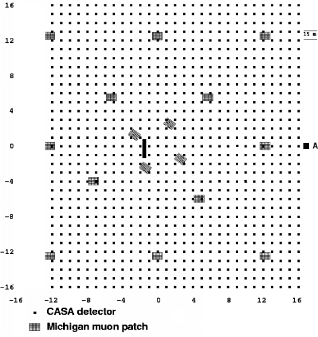
The University of Michigan collaborators designed and built a muon detection array (MIA) to operate in conjunction with CASA. It consists of sixteen “patches,” each having 64 muon counters, buried 3 m below ground at various locations in the CASA array. (See Fig. 1.) Each counter has lateral dimensions 1.9 m $\times$ 1.3 m. Four of the patches, each about 45 m from the center of the array, lie on the corners of a skewed rectangle; four, each about 110 m from the center of the array, lie on a quadrangle with slightly different skewed orientation, and eight lie on the sides and corners of a rectangle with sides $x\simeq\pm 180$ m and $y\simeq\pm 185$ m.

In April of 1991 the CASA/MIA array was partially disabled by a lightning strike which hit one of the few trees on the site. The array was repaired, and an extensive lightning-protection grid installed. The grid consisted of wires strung on poles about 15 feet above the array, traveling in the $x$, $y$, and $x\pm y$ directions. This grid turned out to have significant effect on our choice of parameters for the RF studies.

During the operation of the present experiment, 144 surface Čerenkov detectors [23] were distributed throughout the array. Other additions to the array, which shall not concern us, included a stereographic atmospheric Čerenkov detector (DICE) [24] and an optical facility for communicating with a high-resolution atmospheric fluorescence detector (HiRes) [25] located on a hilltop several miles away.

4.2 Initial RF surveys at CASA/MIA site

In order to determine whether RF pulse detection was feasible at the CASA site, a spectrum analyzer was used to make a broad survey of the RF noise at the CASA site in various frequency ranges and at various locations. It was determined that in the central trailer, the broad-band noise associated with various computers, switching power supplies, and other electronics was so intense that no RF searches could be undertaken. The same was true to a great extent at any position within the perimeter of the lightning-protection grid. Moreover, it was deemed unsafe to erect an antenna above that grid within the perimeter of the array, since any projecting object would defeat the purpose of the grid.

Surveys just outside the array indicated a much quieter RF environment. An antenna was placed about 24 m east of box (16,0), corresponding to $x=263.8$ m, $y=0$ m, and its signal fed into a trailer located about 10 m closer to the array. All further studies were performed using this configuration. (See Fig. 1.) Nonetheless, there still remained a number of identifiable noise sources, which we now describe.

4.2.1 Television and FM broadcast stations

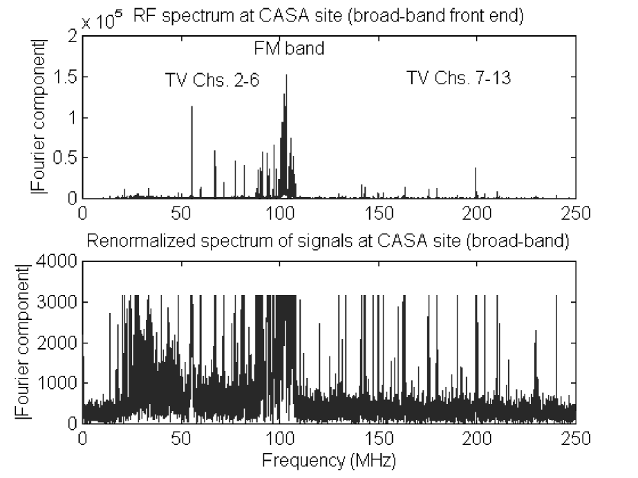
The CASA/MIA site is about 100 km southwest of Salt Lake City, at first sight affording a reasonably quiet RF environment. However, many television and FM stations in Salt Lake City broadcast from a high mountain about 35 km southwest of Salt Lake City, or 65 km northeast of Dugway. These are responsible for a major component of the RF signal in the range which is of greatest interest to us. As an example, we summarize the VHF television stations broadcasting from the above site [26] in Table 1. The video and audio frequencies shown are carrier frequencies. Video signals are modulated with vestigial-sideband modulation, occupying the range from 1.25 MHz below the carrier frequency to about 3.5 MHz above it. A color subcarrier lies 3.58 MHz above the video carrier. Audio signals are frequency modulated with deviation not exceeding 250 kHz so as to remain within the total allotted bandwidth of 6 MHz for each channel. The FM broadcast band, extending from 88 to 108 MHz, is packed with strong signals, with the strongest typically spaced by the 0.8 MHz interval characteristic of inter-station spacing in a large urban area.

Table 1: Television stations broadcasting from site 65 km northeast of Dugway.

Call sign	Channel	Band	Video	Audio	Power
		(MHz)	(MHz)	(MHz)	(kW)
KUTV	2	54–60	55.25	59.75	45.7
KTVX	4	66–72	67.25	71.75	32.4
KSL-TV	5	76–82	77.25	81.75	33.9
KUED	7	174–180	175.25	179.75	155.0
KULC	9	186–192	187.25	191.75	166.0
KBYU-TV	11	198–204	199.25	203.75	162.0
KSTU	13	210–216	211.25	215.75	112.0

4.2.2 CASA noise

The CASA boards contain crystals oscillating at various frequencies, including 16, 20, and 50 MHz. The behavior of a single CASA board was investigated at the University of Chicago. The various clock signals were detected at short distances ($<1$  m) from the board, but a much more intense set of harmonics of 78  kHz emanated from the switching power supplies. These harmonics persisted well above 100 MHz. At 144–148 MHz (monitored using an amateur radio transceiver), they overlapped, leading to intense broad-band noise.

The above signals were considerably less problematic at the RF trailer. During CASA operation the boards’ clock frequencies and some of their harmonics (including 32, 40, and 48 MHz) were detectable. However, noise from the switching power supplies seemed to be at an acceptably low level.

The CASA boards emit powerful RF pulses when digitizing and transmitting data. These pulses constituted a major background to our RF search, and will be discussed in Section 5. The noise arrived through the antenna system and not through the trigger cable or antenna feed cable, as was determined by acquiring data with a dummy load in place of the antenna.

4.2.3 Intermittent narrow-band interference

In addition to persistent RF carriers from TV and FM broadcast stations, intermittent signals would appear from time to time. The strongest of these was traced to local narrow-band FM communications. This signal was so strong that digital filtering methods (to be described below) were powerless to eliminate it. Consequently, any event containing such a signal was discarded for further analysis.

4.2.4 Low-frequency interference sources

Although the majority of survey work dealt with frequencies above 25 MHz, some effort was made to reproduce claims of low-frequency (“LF”) pulses [5], which for our purposes will be taken to involve frequencies below 500 kHz. (The AM broadcast band contains numerous signals above 530 kHz, preventing the study of higher frequencies.) Initial surveys were performed using a Sony SW-7600G all-band portable receiver and an ICOM IC-706 amateur transceiver. However, considerably greater sensitivity was achieved using a Palomar VLF converter which converts the band 10–500 kHz to 3510–4000 kHZ, which was then detected using the IC-706.

The major source of interference at the site was a nondirectional aircraft beacon (NDB) operating at the Dugway airport on 284  kHz. Other NDBs and other LF carriers above about 110 kHz were detectable but considerably weaker. A custom-made filter was procured [27] to suppress the carrier at 284 kHz and signals from the AM broadcast band above 500 kHz. This filter was employed during some of the low-frequency studies to be described below.

4.3 Measurement considerations and initial setup

As mentioned above, the location of the receiving antenna (about 30 m east of the edge of the CASA array, at $x=263.8$ m, $y=0$ m), was dictated by a compromise between proximity to the array and reduction of noise. This noise was carried, to a large extent, by the lightning-protection grid which overlays the array.

It was decided at an early stage to concentrate on the search for horizontally polarized pulses as described in Section 2. Consequently, a broad-band antenna with linear polarization was adopted. Initial surveys were taken with one of the original antennas from the Mt. Chacaltaya experiments [2], which had been preserved from the 1960s. This antenna was a large model manufactured for VHF television reception, with some elements which had been added by the experimenters to improve low-frequency response.

The Mt. Chacaltaya antenna was mounted on a portable searchlight tower attached to a small trailer. The tower could be extended to a height of about 35 feet. The antenna was slightly damaged in a collapse of the tower as a result of improper latching procedures. As insurance against further such incidents, a portable military surplus log-periodic antenna was acquired. This antenna (a Dorne and Margolin model to be described below) was found to have superior response in the frequency range of interest and very robust construction (even surviving a subsequent tower collapse), and was adopted for subsequent studies.

The antenna was mounted on the fully-extended searchlight tower with its center at a height of 35 feet above ground, with the favored direction of reception arriving from the zenith, and with arbitrary azimuthal orientation. Data were taken with two orientations: “East-West” polarization and “North-South” polarization, both referred to magnetic North (14^∘ east of true North [28] at Dugway). In addition, a projecting arm of the mounting bracket was used to suspend a 10-meter-long vertical antenna which was used for the low-frequency surveys.

The bandwidth to be covered by the RF search was not initially specified, but to be determined by experience with survey experiments. Consequently, two main modes were used, a narrow-band mode and a broad-band mode. These are compared in Table 2, where we also list a low-frequency mode used in the LF survey. Their implementation is described in Sec. 4.4.3.

Table 2: Modes of filtering. (a) Suppression at 284 kHz and above 500 kHz in some runs.

Mode	3 dB bandpass (MHz)
Narrow-band	25–35
Broad-band	25–250
Low-frequency	0.05–2.5 (a)

Some previous investigations (e.g., [2] and [3]) were able to detect RF pulses using a “stand-alone” trigger based on the reception of transients alone. This possibility was investigated using a broad-band receiver with filters admitting several different frequency ranges, and demanding coincidences of signals received in a minimum number of channels. It was found that the vast majority of such transients at the Dugway site were not associated with CASA/MIA events; they were probably due to atmospheric discharges. Such “stand-alone” transients, in fact, were found to increase during periods of enhanced atmospheric electrical activity. As a result, our main results concern RF data taken with a trigger based on large CASA/MIA events. We comment further on the possibility of a “stand-alone” trigger for future experiments in Section 6.4.

The trigger was formed at the central CASA/MIA trailer, in a manner to be described in detail below. It was communicated to the RF trailer over RG-59 cable. The electrical length of the cable was found to correspond to a pulse delay of 2.15 $\mu$s. No evidence for pickup of this trigger pulse from the antenna was found. Other methods considered, and rejected in favor of the simpler electrical communication, included optical fiber and infrared sensors.

4.4 Design features

4.4.1 Antenna system

A portable log-periodic antenna manufactured by Dorne and Margolin, Model # DM ARM 160-5, with a nominal response of 30–76 MHz, was acquired from FairRadio Co. in Lima, Ohio, for about $60. (A spare was used for noise studies at the University of Washington.) Overload protection was provided by two 1N4148 diodes of opposite polarity connected across the antenna terminals, leading to a maximum output voltage of about $\pm 0.6$  V. A gas discharge tube manufactured by Alpha/Delta provided lightning protection. Some properties of the antenna are summarized in Table 3.

Table 3: Properties of log-periodic antenna used for RF studies

Nominal frequency range (MHz)	30–76
Usable frequency range (MHz)	28–170
Number of elements	9
Dimensions (m)	$3\times 3$
Feedline RG-58U	60 feet

4.4.2 RF front-end

The RF amplification stage consisted primarily of one or two ZFL-500LN low-noise broad-band preamplifiers manufactured by Mini-Circuits, and for certain runs low-noise preamplifiers manufactured by ANZAC. Specifications of these preamplifiers are summarized in Table 4.

Table 4: Properties of preamplifiers used for RF studies

Manufacturer	Model	DC power	Gain	Frequency
		(V)	(dB)	range (MHz)
Mini-Circuits	ZFL-500LN	13.6	26	DC–500
ANZAC	AM-107	18	10	1–500

4.4.3 Filtering

Table 5 contains a summary of all filters used in the experiment with the exception of the 284 kHz filter [27] described previously. These filters are manufactured by Mini-Circuits; they were obtained with tubular cases fitted with BNC connectors.

Table 5: Filters used in RF data acquisition

Model	Type	3 dB point(s)
		(MHz)
BLP-1.9	Low-pass	2.5
BHP-25	High-pass	25
BLP-30	Low-pass	35
BBP-30	Bandpass	25, 35
BLP-250	Low-pass	250

A typical “narrow-band” configuration described in Table 2 involved feeding the signal from the antenna through the feedline, a BHP-25 filter and a BLP-30 filter with combined 3 dB points of 25 and 35  MHz, a ZFL-500LN preamplifier with 26 dB of gain, a BBP-30 filter with 3 dB points 25 and 35 MHz, another Mini-Circuits ZFL-500LN preamplifier with 26 dB of gain, and a BHP-250 filter to suppress any high-frequency noise. (Some data runs involved permutations of these components. The above configuration was found to minimize feed-through of preamplifier noise. Some runs involved a dual ANZAC preamplifier instead of a ZFL-500LN.)

A “broad-band” configuration involved the same feedline and BHP-25 filter, a single ZFL-500LN preamplifier, and a BLP-250 filter. A “low-frequency” configuration involved the feedline, a BLP-1.9 filter and a ZFL-500LN preamplifier, with a 284 kHz notch filter inserted before or after the BLP-1.9 in some runs. The notch filter also contained a roll-off above 500 kHz.

4.4.4 “Large-event” trigger and design

A trigger based on the coincidence of seven of the eight outer muon “patches” (see Fig. 1) was set to select “large” showers in the following manner. Each muon patch was set to produce a trigger pulse of length 5 $\mu$s and amplitude $-120$ mV when $n$ of its 64 counters registered a minimum-ionizing pulse within $5.2$  $\mu$s of one another. For engineering runs (until 12/28/96), $n$ was set equal to 4, while for later runs it was increased to 5 to favor larger showers and reduce noise. The pulses were then combined in two groups of 4, feeding through two 2X attenuators into two fan-in/fan-outs (to avoid saturation of inputs) and the resulting pulses further combined to produce a summed pulse. This signal was fed to a LeCroy 821 Discriminator, whose output was amplified to an amplitude of about $-6$ V and then sent over RG-59 cable to the RF trailer (see Fig. 1). The trigger pulse at the RF trailer had an amplitude of about $-2.4$  V and a duration of $1~{}\mu$s.

The above trigger was estimated to correspond to a minimum shower energy of somewhat below $10^{16}$ eV, based on the integral rate [29] at $10^{18}$ eV of 0.17/km²/day/sr. At this level good correlation could be established between trigger pulses and events recorded by the CASA data acquisition system.

Only shower radiation that is stronger than 3 $\mu$V$/$m$/$MHz can exceed the average noise level at CASA site by three standard deviations or more [Sec. 4.6]. According to the original Haverah Park results [Eq. (1)], a typical shower that would lead to such radiation is a vertical shower of energy $10^{17}$ eV or higher at a distance of 210 m. If the rate for showers with energy greater than $E$ behaves as $1/E^{2}$, showers above $10^{17}$ eV would be expected to occur with a rate of 17/km²/day/sr. Since RF detection relies on muon triggering, the antenna can only detect radiation from those showers whose cores pass inside the rectangle of the array. Just about 0.06 km² of the array area lies inside the 210 m radius from the antenna. With the solid angle of observation limited by a zenith angle of 50^∘, one expects about 2.25 detectable shower pulses per day.

4.4.5 Data acquisition

A Tektronix TDS-540B digitizing oscilloscope registered filtered and preamplified RF data on a rolling basis. These data were captured and stored on hard disk using a National Instruments GPIB interface upon receipt of a large-event trigger. Data were taken using various computers at different times, allowing for analysis both at the University of Washington and at Chicago. The Washington system used a Macintosh Quadra 950 running Labview, with a latency time of about 8 seconds between events, while the Chicago system used either a Dell XPS200s desktop or a Dell Latitude LM laptop running a C program adapted from those provided by National Instruments, with a latency time of about 2 seconds. Each trigger caused 50 $\mu$s of RF data, centered around the trigger and acquired at 1 GSa/s, to be saved.

4.4.6 Rates and off-line processing

The total trigger rate ranged between about 20 and 50 events per hour, depending on the value of $n=4$ or $5$ of muon counters chosen to generate a patch trigger pulse and on intermittent sources of noise sometimes present in the trigger system. Concurrently, the CASA on-line data acquisition system was instructed via a special program called MUTRIG to write files of events in which at least 7 out of the 8 outermost muon patches produced a patch pulse. These files, one for each CASA run, typically overlapped with the records taken at the RF trailer to a good but not perfect extent [30] as a result of occasional noise on the trigger line. Moreover, an undiagnosed timing problem occasionally caused the loss of a muon trigger pulse for certain large events recorded by MUTRIG.

4.4.7 Off-line overload rejection

Events were typically recorded at a gain such that the maxima and minima corresponded to about 2/3 of the dynamic range of the oscilloscope’s 8-bit data acquisition system (ranging from $-128$ to $127$ digitization units). Local intermittent monochromatic RF signals occasionally saturated this dynamic range. Such events were rejected off-line by discarding any cases in which the maxima and minima exceeded 100 digitization units. In the configuration used for the final bounds on pulse amplitudes, corresponding to an oscilloscope setting of 5 mV per division of 25 digitization units, we thus rejected all signals corresponding to preamplifier peak outputs greater than $\pm 20$ mV. In some cases, with oscilloscope settings of 20 mV per division, we rejected signals with preamplifier peak outputs greater than $\pm 80$ mV. In all cases these voltages were well below the manufacturer’s specified limit of $\pm 400\sqrt{2}$ mV (3 dBm), and within a satisfactorily linear range of preamplifier response.

4.4.8 Calibration

The average gain $G_{ant}$ of the antenna in its forward direction rises from about 3 dBi (decibels with respect to an isotropic radiator) at 30 MHz to a peak of about 5 dBi at 50 MHz, slowly decreasing to 4 dBi at 76 MHz [31]. We shall take an average gain of 4 dBi ($G_{ant}=2.5$) over the frequency range of interest.

More precise calibration would involve modelling of the gain pattern using a program such as EZNEC [32], and integrating over directions of expected signal arrival. This modelling also would have been useful in order to emulate the frequency-dependent phase distortion induced by the antenna, but it was not found possible to obtain a sufficiently close fit to the antenna’s measured standing-wave-ratio characteristics to take such a model seriously. Certainly this point should be addressed in any future studies. One might also utilize sources of known strength such as amateur radio satellites broadcasting on 29.4 MHz, FM and television stations, and galactic and solar noise. The existing data contain signals from FM and television stations broadcasting near Dugway, some of whose field strengths are well enough known that they may be usable for calibration. Alternatively, for future work it would be helpful to calibrate antennas on an antenna range at some distance from an impulse generator, broadcasting through a broad-band antenna with already-determined characteristics.

4.5 Signal processing

4.5.1 Fourier methods

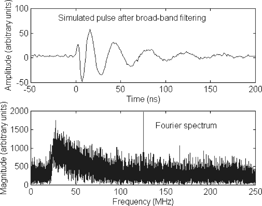
In order to remove strong Fourier components associated with signals which were approximately constant over the duration of each data record, a short MATLAB routine was written to perform the fast Fourier transform of the signal and renormalize the large Fourier components to a given maximum intensity. Fig. 2 shows the fast Fourier transform of a typical RF signal before and after this procedure was applied. In each case the data were acquired using the “wide-band” filter configuration, whose response cuts off sharply below 23 MHz.

Figure 2: Top panel: Fourier spectrum (in arbitrary units) of RF signals acquired at Dugway site using high-pass 25 MHz and low-pass 250 MHz filters. Prominent features include video and audio carriers for TV Channels 2, 4, 5, 7, and 11 (see Table 1 for frequencies), and the FM broadcast band between 88 and 108 MHz. Bottom panel: Fourier spectrum (same vertical scale) after renormalization of large Fourier components to a magnitude chosen here to be $3.16\times 10^{3}$. In practice best sensitivity to transients was obtained by renormalizing to a magnitude of $10^{3}$.

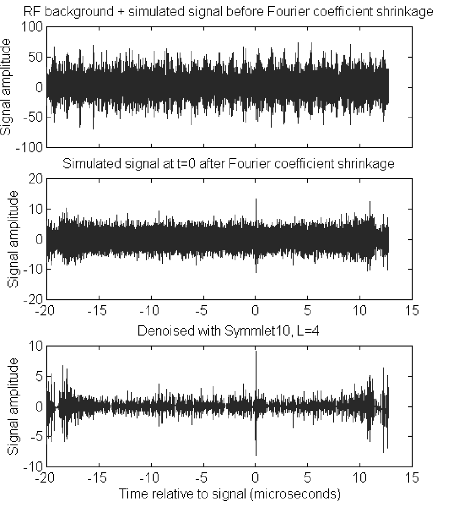
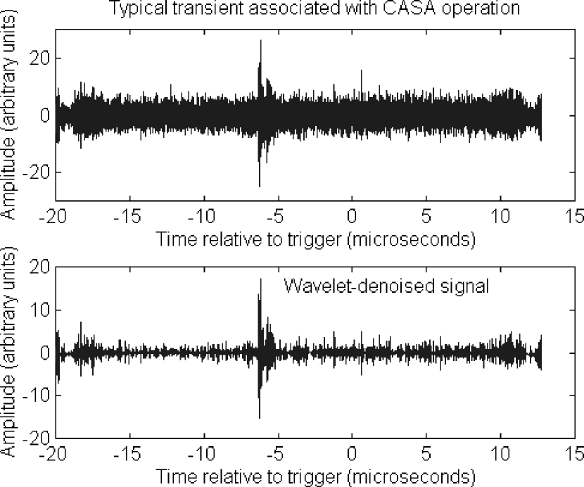
The effect of digital filtering on detectability of a transient is illustrated in Fig. 3. The top panel shows the RF record whose Fourier transform was given in Fig. 2, on which has been superposed a simulated transient of peak amplitude 14.5 digitization units. (The data acquisition scale ranges from $-128$ to $+127$ digitization units; one scale division on the oscilloscope corresponds to 25 units.) The transient is invisible beneath the large amplitude associated with television and FM radio signals. The middle panel shows the result after application of the Fourier coefficient shrinkage algorithm.

Figure 3: Effect of Fourier coefficient shrinkage on detectability of a transient. Top panel: raw RF record (in arbitrary units) with simulated signal superposed. Middle panel: record (same scale) after Fourier coefficient shrinkage. Here a maximum Fourier coefficient magnitude of $10^{3}$ (in the units of Fig. 2) has been imposed. Bottom panel: the same record after denoising with a 10-point symmlet level $L=4$ routine [35].

The event in Figs. 2 and 3 consisted of 32,768 data points obtained at a 1 ns sampling interval, with the trigger at the 20,000th point. The frequency resolution in the fast Fourier transform is thus 500 MHz (the Nyquist frequency) divided by 16,384, or about 30 kHz. This permits rather fine distinction between frequencies containing a strong carrier and those which correspond to its weaker sidebands. At the same time, it permits time resolution to be preserved, allowing for the examination of rather rapid transients. To the extent that these transients do not contain Fourier coefficients exceeding a pre-determined threshold, they should be relatively unaffected by the shrinkage algorithm in the absence of interfering signals. However, since at Dugway signals in nearly the whole FM band (88–108 MHz) exceed the threshold, some distortion is unavoidable using such a method. In obtaining bounds on pulse amplitudes we therefore employ a method involving the comparison of Fourier power in a given time window with the average power obtained over the whole data record for each Fourier component. This method is described below.

4.5.2 Time-frequency analyses

One can perform a fast Fourier transform using a small time window (typically 1024 ns) which is advanced sequentially through the data record, typically in steps of 100 ns. The frequency resolution of any given “snapshot” is then 500 MHz divided by (typically) 512, or a bit better than 1 MHz. A two-dimensional display of time vs. frequency then allows one to distinguish short transients (with components over many frequency bins) from continuous RF sources (with components in narrow frequency ranges over the entire time record). One such plot appears in Fig. 11, Sec. 5.3.1, below. In practice one may wish to suppress frequencies corresponding to the whole FM band and known TV stations, so as not to overload the dynamic range of the display. An alternative method [33] is to renormalize each point in time–frequency space so that deviations from the average in each frequency bin are displayed. This method is described further in Sec. 5.2. It was used for the main part of data analysis.

4.5.3 Wavelet techniques

The wavelet package Wavelab [34] contains a denoising routine which was adapted for our purposes. While an exhaustive search for optimized methods was not performed, good results in reducing noise levels were obtained using a 10-point symmlet routine with level $L=4$ [35]. An example of a denoised signal is shown in the bottom panel of Fig. 3. Here a simulated signal of positive peak amplitude 14.5 digitization units has been added to an RF record otherwise free of transients. The effect of wavelet denoising is to reduce the amplitude of random high-frequency fluctuations while preserving edge effects such as transients.

4.6 Signal simulation

We wished to quantify the improvement associated with each method of signal processing. We thus simulated the expected signal by generating it using an arbitrary waveform generator, feeding it through the same preamplifier and filter configurations used for data acquisition, and superposing it on records otherwise free of transients. We successively reduced the amplitude of the superposed test signal until it could not be distinguished from random noise peaks, thereby obtaining an estimate of sensitivity.

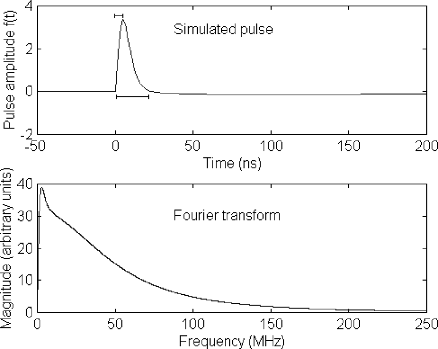
A Hewlett-Packard Arbitrary Waveform Generator was used to generate signals whose characteristics are illustrated in Fig. 4. These signals were taken to have the form $f(t)=\theta(t)At^{2}(e^{-Bt}-Ce^{-Dt})$ with the coefficient $C$ chosen so that $f(t)$ has no DC component, and $D$ corresponding to a long duration of the negative-amplitude component. For all pulses we chose $D=B/20$, so that $C=(8000)^{-1}$ cancels the DC component. The Fourier components of the test pulse fall off smoothly with frequency. The initial $t^{2}$ behavior was chosen so that both the test pulse and its first derivative vanish at $t=0$, as might be expected for a pulse from a developing shower.

The simulated pulses are summarized in Table 6. Instead of quoting the value of $A$, we quote the maximum positive value of the pulse, both before and after filtration and preamplification. These values of $V_{\rm pk}$ reflect choices for convenience in display on the oscilloscope, and are otherwise arbitrary.

Figure 4: Analytic depiction of typical pulse presented to filter-preamplifier configuration. Top panel: time dependence of pulse $f(t)=\theta(t)t^{2}[e^{-0.4t}-e^{-0.02t}/8000](t$ in ns); bottom panel: Fourier spectrum of pulse (calculated analytically). In the top panel, the short bar above the pulse denotes $\delta$, the time difference between onset and maximum, while the longer bar below the pulse denotes $\Delta$, the duration of the positive component.

Table 6: Parameters of test signals. $\delta$ is the time between pulse onset and maximum, while $\Delta$ is the duration of the positive component of the pulse. $V_{\rm pk}$ is the peak (positive) input voltage to the filter-preamplifier configuration. The letter after the peak voltage denotes (a) narrow-band (25-35 MHz) or (b) broad-band ($>25$ MHz) configuration (see Sec. 4.4.3). $V_{\rm out}$ is the peak-to-peak amplitude of the pulse emerging from the filter-preamplifier configuration. $S$ is the scale factor with which data were recorded on oscilloscope.

$B$	$\delta$	$\Delta$	$V_{\rm pk}$	$V_{\rm out}$	S
(ns-1)	(ns)	(ns)	(mV)	(mV)	(mV/div)
0.8	2.5	12	1.2 (a)	86	20
			6.0 (b)	124	20
0.4	5	24	0.7 (a)	70	20
			1.3 (b)	21	5
0.2	10	47	0.7 (a)	71	10
			7.0 (b)	67	10
0.1	20	95	1.5 (a)	75	10
			7.6 (b)	32	5

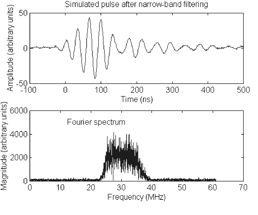
The shape of the pulse of Fig. 4 is affected by preamplification and filtration as shown in Figs. 5 (broad-band) and 6 (narrow-band). The noise in these figures and the sharp feature at 125 MHz in Fig. 5 are associated with the system used to generate the test pulse, and the fact that the Fourier transform is taken over a much longer time than the duration of the pulse.

Systematic studies of signal-to-noise ratios have been performed so far only for the simulated pulses with $\delta=5$ ns applied to a broad-band front end [(b) in Table 6]. The value of $\delta$ is a measure of the distance $R$ of closest approach of the shower core [3]. This choice corresponds to a typical distance $R\simeq 200$ m. A typical pulse of this type gave a front end output of 21 mV peak-to-peak, acquired at an oscilloscope sensitivity of 5 mV per division. Each division corresponds to 25 digitization units, so the peak-to-peak range is about 104 digitization units, or slightly less than half the dynamic range (255 units, or 8 bits). Positive and negative peaks are thus about 52 digitization units each.

The stored test signal is then multiplied by a scale factor and added algebraically to a collection of RF records in which, in general, randomly occurring transients will be present. One then inspects these records to see if the transient can be distinguished from random noise.

Figure 5: Test pulse of Fig. 4 after broad-band filtration ($>25$ MHz) and preamplification. Top panel: time dependence of pulse; bottom panel: Fourier spectrum of recorded pulse for $-20~{}\mu{\rm s}\leq t\leq 12.768~{}\mu$s.

For the broad-band data we estimated that pulses with input voltages corresponding to about 1/5 the original test pulse amplitude can be distinguished from average noise (not from noise spikes!). Since the original test pulse had a peak value of 1.3 mV, this corresponds to sensitivity to an antenna output of about $V_{\rm pk}\simeq 260~{}\mu$V. The ability to detect such a pulse with an effective bandwidth of about 30 MHz corresponds to a threshold sensitivity at the level of order $3~{}\mu$V/m/MHz (see Appendix B).

Preliminary studies of simulated pulses applied to the narrow-band front end suggest a considerably poorer achievable signal-to-noise ratio, despite the expectation that the signal should have a large portion of its energy between 23 and 37 MHz. It appears difficult to detect a pulse from the antenna below about 0.7 mV, which for a bandwidth of 14 MHz corresponds to a threshold sensitivity of $7~{}\mu$V/m/MHz, not sufficient for our purposes. Studies of possible improvements of the analysis algorithm for the narrow-band data are continuing.

Figure 6: Test pulse of Fig. 4 after narrow-band filtration (25–35 MHz) and preamplification. Top panel: time dependence; bottom panel: Fourier spectrum of recorded pulse for $-20~{}\mu{\rm s}\leq t\leq 12.768~{}\mu$s.

5 Results

Table 7: Triggers associated with CASA operation taken under various conditions.

Front end	Macintosh	Dell	Total
Narrow-band	5849 (139.78 h)	1952 (48.97 h)	7801 (188.75 h)
Broad-band	9603 (272.57 h)	5416 (121.62 h)	15019 (394.18 h)
Low-frequency	0	505 (17.67 h)	505 (17.67 h)
Total	15452 (412.35 h)	7873 (188.25 h)	23325 (600.6 h)

Table 8: Broad-band data recorded on Macintosh Quadra.

Antenna	CASA	CASA	Partial	Total
Polarization	HV on	HV off	CASA HV	events
East-West	4966 (119.03 h)	859 (21.88 h)	1957 (53.08 h)	7782 (194.0 h)
North-South	696 (30.53 h)	582 (23.25 h)	543 (24.78 h)	1821 (78.57 h)
Total events	5662 (149.57 h)	1441 (45.14 h)	2500 (77.87 h)	9603 (272.57 h)

5.1 Event sample

More than 20000 triggers, obtained under various conditions of filtering, preamplification, and noise reduction during the period February 1997 – March 1998, are summarized in Table 7. Events recorded on a Macintosh Quadra 950 and those recorded on a Dell LM Latitude laptop computer are listed separately because the power supply of the latter introduced spurious transients. Our initial analysis concentrated on data taken with the Macintosh. For reasons mentioned above, we consider only the broad-band data at this time. Thus, our usable sample consists of over 9000 CASA triggers. In addition, periodic forced triggers were taken to monitor noise activity not associated with CASA operation.

The broad-band data recorded on the Macintosh Quadra, summarized in Table 8, are subdivided into several categories. Data were taken with both East-West (EW) and North-South (NS) antenna polarizations. Moreover, since noise from CASA boxes was found to be a significant source of RF transients, data were taken with some or all CASA boxes disabled by turning off the high voltage (HV) supply to the photomultipliers. Even when HV is supplied only to boxes that are further than 100 m from the antenna, the RF transients from these boxes provide a strong background. (See the discussion in Sec. 5.2 and Fig. 10 below.) One is unlikely to distinguish the RF pulses of the showers from this noise. Therefore, we concentrated on data with CASA HV off, with 859 triggers taken with EW antenna polarization (21.88 active hours) and 582 triggers taken with NS antenna polarization (23.25 active hours). For subsequent sensitivity calculations, a subset of data was used consisting of 756 EW triggers (17.25 hours) and 528 NS triggers (21.12 hours). The remaining data with CASA HV off occurred in very short runs (52 EW triggers and 19 NS triggers) or was contaminated by local VHF communication signals (51 EW triggers and 35 NS triggers). Data with CASA HV on or partially disabled were not used for the present analysis.

Figure 7: Top panel: intensity-vs.-time plot for maxima of 880 pulses recorded in 698 triggers in January 1998 with CASA HV supplied to all stations. Bottom panel: time distribution of transients. All events recorded with East-West antenna polarization.

5.2 Characterization of transients associated with CASA operation

Several means were used to characterize transients. One method with good time resolution involved the shrinkage of large Fourier coefficients to a fixed maximum intensity, as in Figs. 2 and 3. Another, which we have used for results to be presented below, involves generation of a time-vs.-frequency intensity plot by Fourier-transforming 1024-ns subsets of the 50 $\mu$s data record, spaced by 100 ns steps. Since the data are sampled at 1 ns intervals, the frequency resolution of this method is thus about 1 MHz. The intensity $S(\nu,t)$ is then averaged over time $t$ for each frequency $\nu$ to form an average intensity $\bar{S}(\nu)$. The quantity $S(\nu,t)/\bar{S}(\nu)$ is an estimate of the degree to which the intensity at a given frequency $\nu$ and time $t$ exceeds the average over the $50~{}\mu$s sampling time. We then average $S(\nu,t)/\bar{S}(\nu)$ over $\nu$ to search for events in which the average intensity at a given time is exceeded in many simultaneous frequency bands.

Figure 8: Top panel: intensity-vs.-time plot for maxima of 824 pulses in 691 triggers recorded in January 1998 with CASA HV disabled. Bottom panel: time distribution of transients. All events recorded with East-West antenna polarization.

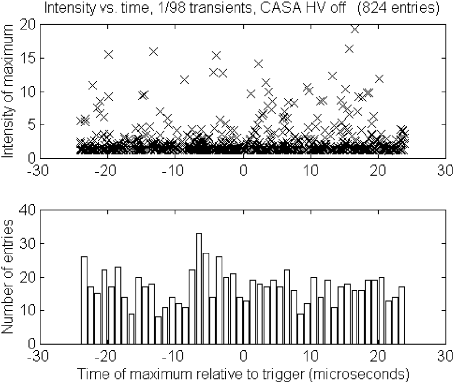
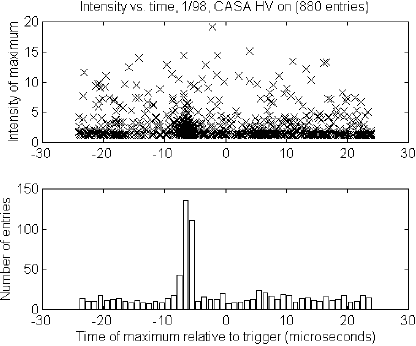
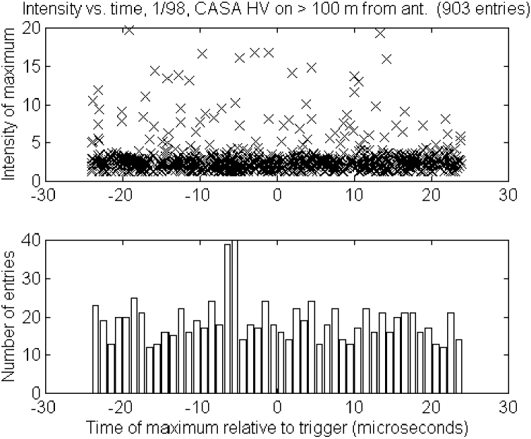
One can then search for peaks of each data record (there may be several peaks in a record), plotting intensity of their maxima against time relative to the trigger. One such plot is shown in Fig. 7 for a data run in which CASA HV was delivered to all boxes. A strong accumulation of transients, mostly with intensity just above the arbitrarily chosen threshold (mean + 3 $\sigma$ for each trigger sample), is visible at times $-5$ to $-7~{}\mu$s relative to the trigger. In a comparable plot for a run in which CASA HV was completely disabled (Fig. 8), only a small accumulation at times $-6$ to $-7~{}\mu$s is present. This excess appears due to transients with predominantly high-frequency components (over 100 MHz). Since signal pulses are expected to have more power below 100 MHz (see Fig. 5, bottom) we believe that this accumulation is not due to shower radiation, but most likely arises from the muon patches, one of which is within 75 m of the antenna.

Figure 9: Signal of a typical transient associated with CASA operation. Top panel: before denoising; bottom panel: after denoising.

A typical transient occurring in a run with CASA HV on is shown in Fig. 9. The transients are highly suppressed (though not in all runs) when CASA boxes within 100 m of the antenna are disabled, as shown in Fig. 10.

The time distribution of pulse maxima above an arbitrary threshold for 880 pulses detected with CASA HV on (one run from January 1998 composed of 698 files of data) is shown in the bottom panel of Fig. 7. The mean arrival time is about $6~{}\mu$s before the trigger, with a distribution which is slightly broader for pulses arriving earlier than the mean. This broadening may correspond to some jitter in forming the trigger pulse from the sum of muon patch pulses.

As mentioned earlier, the time for the trigger pulse to propagate from the central station to the RF trailer was measured to be $2.15~{}\mu$s. One expects a similar or slightly greater travel time for pulses to arrive from muon patches to the central station (see Fig. 1). Moreover, the muon patch signals are subjected to delays so that they all arrive at the central station at the same time for a vertically incident shower. Thus, the peak in Fig. 7 is consistent with being associated with the initial detection of a shower by CASA boxes. This circumstance was checked by recording CASA trigger request signals simultaneously with other data; they coincide with transients such as those illustrated in Fig. 9 within better than $1/2~{}\mu$s.

Figure 10: Top panel: intensity-vs.-time plot for maxima of 903 pulses recorded in 620 triggers in January 1998 with CASA HV disabled for boxes within 100 m of antenna. Bottom panel: time distribution of transients. All events recorded with East-West antenna polarization.

The RF signals from the shower are expected to arrive no later than, or at most several hundred nanoseconds before, the transients associated with CASA operation. They would propagate directly from the shower to the antenna, whereas transients from CASA stations are associated with a longer total path length from the shower via the CASA station to the antenna. There will also be some small delay at a CASA station in forming the trigger request pulse. Thus, we expect a genuine signal also to show up around 6–7 $\mu$s before the trigger.

The time coincidence of the CASA RF transients and the shower signals is a significant obstacle to detecting genuine pulses. Therefore, data with CASA HV on or partially disabled were not used for the present analysis. As we show below in Secs. 5.3.1–5.3.3, no significant peak is visible around 6–7 $\mu$s before the trigger for data recorded with CASA HV off. The upper limit on the rate of events giving rise to such a peak can be used to set a limit on RF pulses associated with air showers, as we demonstrate in Sec. 5.3.4.

5.3 Estimated upper bounds on broad-band signals

As mentioned in Sec. 5.1, the following discussion is based on 17.25 active hours of data accumulation with EW antenna polarization and 21.12 hours with NS antenna polarization. The small duration of this subset of data limits its sensitivity to RF signals from the shower.

5.3.1 Criteria used to distinguish noise and signal transients

The main difficulty associated with pulse detection is that signal pulses are not easily distinguishable from large spurious pulses originating from atmospheric discharges. Both air shower pulses and these background noise pulses can considerably exceed the average noise level. Several criteria can be used to distinguish signal pulses from noise. The conventional criteria of the previous studies have been that the pulse should be (1) larger than the average noise level by some small specified amount, (2) time coincident with shower particles, and (3) bandwidth limited [3]. All these criteria were adopted in this study and one more has been added: The pulse should have approximately uniform distribution over frequency within its limited bandwidth [see (c) below].

We now note the particular criteria used to distinguish signal pulses in this study.

Figure 11: Simulated pulse (horizontal band at $0~{}\mu s$) and noise transient (horizontal band at about $15~{}\mu s$) on a 2-d plot of intensity (grayscale) vs. time (vertical axis) and frequency (horizontal axis). Unlike the simulated pulse, the noise transient contains high frequency components. Grayscale: black color denotes the highest intensities, white the lowest. Vertical bands indicate continuous RF sources in the 54–200 MHz range.

(a) Pulse magnitude

Continuous RF interference in each frequency channel was removed by advancing a moving 1024-ns window in 100 ns steps through the data record to produce a time-vs.-frequency plot [Sec. 4.5.2] and then using the averaging procedure described in Sec. 5.2. Defining the average signal as 1 (in arbitrary units), the pulse threshold in each event was taken to be the larger of either (a) the mean plus three standard deviations, or (b) 1.8 (in the same units). The former permitted removal of an average noise level; the latter discriminated against small noise transients. The final result was not affected by the choice of the factor 1.8 since the subsequent analysis [Sec. 5.3.3] used a considerably higher threshold.

(b) Limited bandwidth of pulses

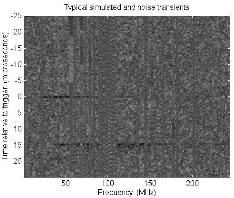
Broad-band filtering limits the frequency range to 23–250 MHz [Sec. 4.4.3]. The investigation of the simulated pulses on a 2d-plot of intensity vs. time and frequency suggested that, unlike some strong noise transients, the signal pulse intensity declines drastically in the range above approximately 100 MHz (Fig. 11). This feature is consistent with theoretical predictions for the shower pulse spectrum [36]. It can be chosen as a criterion for separating noise and signal transients. The ratio of mean intensities averaged over 23–100 MHz relative to that averaged over 100–250 MHz was found to be greater than 1 for all simulated pulses and smaller than 1 for some noise pulses.

One can consider intensities averaged over the part of the whole frequency range. To facilitate separation of signal transients it is preferable to choose a region where the signal-to-noise ratio is particularly large. Unfortunately, the whole region from 23 MHz to 100 MHz cannot be effectively used for this purpose. The 54–82 MHz range is occupied by TV channels 2, 4 and 5, which leads to high noise levels. The same is true for the whole FM band (88–108 MHz) [Sec. 4.2.1]. However, this is not the case in the 24–54 MHz range. The noise level in this range is mostly uniform, and simulated pulse intensities are particularly large there in comparison with the noise level. The assumption that the 24–54 MHz range provides the best signal-to-noise intensity ratio has been tested. The results for this range have been compared with the ones obtained in the 10–54 MHz and 24–86 MHz regions and were found to be superior. Subsequently, the range of 24–54 MHz was chosen as the main region of investigation.

After that, it was natural to choose the ratio of mean intensities averaged over 24–54 MHz relative to that averaged over 55–250 MHz at the moment of each pulse as a criterion for discriminating noise and signal pulses. For all simulated pulses this ratio was greater than 1. All pulses for which this ratio was smaller than 1 were assumed to be noise transients and discarded. Also, a ratio parameter threshold other than 1 can be chosen. The parameters that provided best results were found to lie between 1.4 and 1.8 [Section 5.3.4].

(c) Approximately uniform distribution of pulse intensity over frequency in the 24–54 MHz range

The most intense noise transients that met criteria (a) and (b) were found to display a peculiar feature: Their intensities were concentrated in a small region of approximately 10 MHz width somewhere in the 24–54 MHz range. This non-uniformity allowed such pulses to be ruled out. If the pulse intensity, integrated over any 9 MHz width window (in the 24–54 MHz range), was greater than the intensity integrated over the remaining 21 MHz, then such a non-uniform pulse was discarded as a noise transient. The reason for choosing a 9 MHz width window was that most simulated pulses passed this test, while many noise transients did not.

The effectiveness of these three criteria is illustrated in Table 9. For simulated pulses that are stronger than 3.43 $\mu$V/m/MHz the combination of criteria (b), (c) and a very high intensity threshold provides a $84.1/4.75\approx 18$ times increase for their relative fraction with respect to noise transients.

Table 9: Fraction of noise pulses passing criterion (a) that can also pass criteria (c) and (b) with ratio parameter threshold of 1.4, and whose maximum intensities are larger than some very high intensity threshold. Fraction of simulated pulses of different strengths (in $\mu$V/m/MHz), that can pass criteria (c) and (b) with ratio parameter threshold of 1.4, and whose maximum intensities (after they are superimposed on noise) are larger than the same high intensity threshold. The strengths of the pulses are chosen to be stronger than $1/n$ times an original test pulse amplitude of 13.7 $\mu$V/m/MHz, $n=2,3,4,\ldots,7$.

		Simulated pulses that are stronger than
	Noise pulses	6.85	4.57	3.43	2.74	2.28	1.96
		$\mu$V/m/MHz
North-South	4.47%	94.1%	91.7%	85.2%	66.9%	47.7%	36.7%
East-West	4.75%	98.8%	93.4%	84.1%	67.7%	48.7%	41.4%

5.3.2 Method outline

The time coincidence of the pulse with air shower particles implies that a signal pulse should be looked for in the range between $-7$ and $-6~{}\mu s$ [Sec. 5.2], which will be referred to in what follows as “the interesting time bin”. It is important to note that the aforementioned test criteria are not efficient if applied only to the pulses found in this time bin. Indeed, some noise pulses in the bin meet all criteria. Hence, accepting all the pulses that pass this test would not guarantee that signal pulses are present among them at all. We developed a different approach.

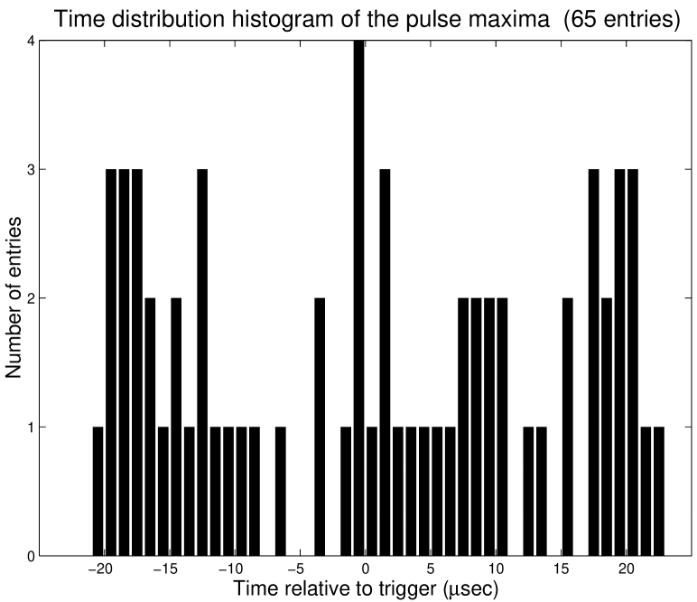
The time distribution of noise pulses is assumed to be uniform. Hence, the following technique can be adopted. First, the time distribution histogram of the pulse maxima (from the whole data run) can be plotted. Then, in the absence of signal pulses, the number of pulses in a time bin should obey a Poisson distribution with the average being equal to the average pulse number per bin. Suppose that an accumulation of pulses in the interesting time bin $(-7,-6)~{}\mu s$ is large enough that its probability according to the Poisson distribution is less than 5%. Then this signifies the presence of signal pulses with a confidence level of 95%.

Thus, a sufficiently large relative accumulation of entries in the interesting time bin was adopted as a key criterion in search of signal pulses.

5.3.3 Detailed description

Figure 12: Intensity vs. time plot for maxima of transients in 756 files of data with East-West antenna polarization and CASA HV off. The horizontal line denotes the threshold taken to lie at the level of the 17th strongest pulse. Only criterion (a) of Sec. 5.3.1 was employed, resulting in a large (1367) number of entries.

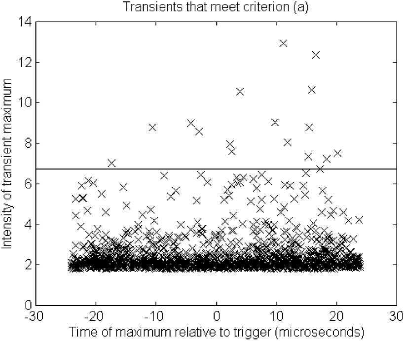
A routine was designed to scan all events in the whole data run and select the transients that passed criterion (a) in Sec. 5.3.1. The ratio parameter (see above) and uniformity parameter [1, if criterion (c) was satisfied, and 0, if not] were recorded along with time relative to the trigger and intensity of a transient. The intensity vs. time plot of pulse maxima selected in this manner for the data taken with East-West antenna polarization is shown in Fig. 12.

In order to be detectable, signal pulses should be stronger than the average noise transient, whose intensity equals 2.5 as a result of the specific criteria imposed. Hence, it is reasonable to set the intensity threshold sufficiently high to enhance the relative accumulation in the $(-7,-6)~{}\mu s$ time bin. One can set a high threshold and determine the number of pulses that pass through it. Divided by number of bins, this number gives the average pulse number per bin. This, in turn, can be used as an average value of the Poisson distribution to determine whether the probability of the observed accumulation in the interesting bin is less than 5%.

The effectiveness of this technique depends on the choice of intensity threshold. If the threshold is too low, the histogram includes many noise pulses. Then, the signal pulse accumulation in the interesting time bin becomes relatively small to be distinguished from statistical fluctuations. If the threshold is too high, it may cut out some signal pulses and the remaining ones may not make up a significant accumulation. The choice of the optimum threshold is discussed below.

Optimum intensity threshold.

Suppose we look for an accumulation of 2 or more entries. Such an accumulation is significant (i.e. its probability is $\leq 5\%$) if the average number of pulses per bin is about 0.355. Indeed, according to Poisson distribution, $P(\mbox{0 entries})=\exp(-0.355)\approx 0.701$, $P(\mbox{1 entry})=0.355\cdot\exp(-0.355)\approx 0.249$, so $P(\mbox{$\geq 2$ entries})=1-0.701-0.249=0.05$. Since the standard histogram used in the study contained 48 bins (of 1 $\mu s$ each), the average value of 0.355 pulses per bin would correspond to a total number of $0.355\cdot 48\approx 17$ pulses. These considerations suggest that the intensity threshold would not have some fixed value but would correspond to the intensity of the 17th strongest pulse [see Fig. 12]. Then, the total number of entries in the histogram is 17 and the average number of entries per bin is about 0.355. So, 2 or more entries in the interesting bin, if observed, would have the probability of 5% and would reveal the presence of signal pulses with 95% CL.

Table 10: Significant accumulation of entries in the interesting time bin and the corresponding optimum threshold (calculated according to Poisson distribution).

Number of entries in the interesting time bin one is looking for	Average number of entries per bin at which the probability of this accumulation becomes $\leq 5\%$	Corresponding total number of entries in the 48 bin histogram (optimum threshold)
2	0.355	17
3	0.817	39
4	1.366	65
5	1.970	94
6	2.613	125
7	3.285	157
8	3.980	191
9	4.695	225
10	5.425	260
11	6.170	296
12	6.924	332
13	7.690	369
14	8.464	406
15	9.245	443
16	10.035	481
17	10.832	519
18	11.635	558
19	12.443	597
20	13.256	636

Naturally, the probability of 3 or more entries would be even smaller and approximately equal to $P(\mbox{$\geq 3$ entries})=P(\mbox{$\geq 2$ entries})-P(\mbox{2 entries})=0.05-\frac{0.355^{2}}{2!}\exp(-0.355)\\ \approx 0.006$. That is, if such an accumulation were observed, the presence of signal pulses could be claimed with a confidence level of 99.4%. However, in reality it is unlikely that signal pulses could be detected with such a confidence level. To improve the detection chances, it is advantageous to lower the threshold to the 39th strongest pulse. This sets the average number of entries per bin to $39/48\approx 0.813$ and makes the probability of 3 entries equal to 5%. The threshold of the 39th strongest pulse is the lowest one that still guarantees a confidence level of at least 95%.

Thus, the convenient threshold depends on the significant accumulation number one is looking for. For any particular accumulation, one can choose the optimum threshold which would guarantee a confidence level of at least 95%. The significant accumulation number and the corresponding optimum threshold can be found in Table 10.

This method did not reveal any significant accumulation in the interesting time bin. So far, however, only criterion (a) and intensity thresholds were applied to detected pulses. As was already mentioned in the beginning of this Section, the ratio and uniformity parameters were recorded for each simulated or noise pulse. This made it easy to impose criterion (b) with different ratio parameter thresholds and criterion (c). Their application should have increased the ratio of signal pulse number to noise pulse number. Unfortunately, no significant accumulation has been detected (see Fig. 13). This means that signal pulses are quite rare, so that the resulting accumulation is not significant. However, upper limits can be placed on the rate (in h^-1) of signal pulses that are stronger than some fixed value. This will be our aim for the next subsection.

Figure 13: Time distribution histogram for maxima of the 65 strongest pulses extracted from 756 files of the EW data with (a), (b) and (c) imposed. The ratio parameter threshold for criterion (b) is 1.4. An accumulation of 4 or more pulses in the (–7,–6) $\mu$s bin would signify the presence of signal pulses. Such an accumulation was not detected.

5.3.4 Upper limits on the rate

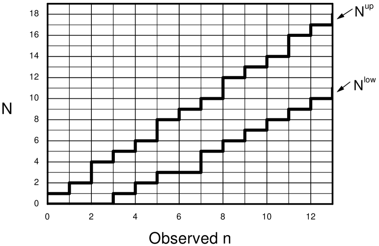
The total number $n$ of observed transients in the interesting time bin consists of both noise and signal events. The former are Poisson-distributed with known average $\mu$. The latter obey a binomial distribution with a known probability $P$ to pass thresholds and an unknown total number $N$ of signal events contained in the run. Using a unified approach to the statistical analysis of small signals [37], we construct 95% confidence belts for unknown $N$. For any choice of imposed thresholds, the lower end of confidence intervals is 0, i.e. only upper limit on the total number of signals in the run can be placed.

Probability $P_{s}(k)$ that the interesting bin contains $k$ signal events.

Formula (1) [Section 3] shows that ${\cal E}_{\nu}$ is directly proportional to primary energy $E_{p}$. The differential rate of primaries is known to fall approximately as $1/E_{p}^{3}$ [29]. Similarly, the differential rate of ${\cal E}_{\nu}$’s should be proportional to $1/{\cal E}_{\nu}^{3}$.

Simulated pulses of different strength ${\cal E}_{\nu}$ greater than some ${\cal E}_{\nu}^{0}$ can be added to each event of the data run. To simulate the expected rate for ${\cal E}_{\nu}$, a Monte-Carlo simulation was performed in such a way that the number of added simulated pulses with strength ${\cal E}_{\nu}$ falls as $1/{\cal E}_{\nu}^{3}$.

Each event underwent the averaging procedure described in Sec. 5.2. The averaged intensities of simulated pulses were compared to the values of the 17th (or 39th, 65th, etc.) strongest noise pulse of the initial data (without added simulated pulses). The fraction of simulated signal pulses that were higher than this threshold gives the probability $P$ for a signal pulse with strength greater than some ${\cal E}_{\nu}^{0}$ to exceed this threshold. We determined the value of $P$ as a function of ${\cal E}_{\nu}^{0}$, the intensity threshold, and the set of criteria ((a), (b),(c), or some combination of them) imposed on both noise and signal pulses. Then, these values were used to make an analytical estimate of the probability to detect a significant accumulation number of entries in the interesting bin.

By making an assumption for the total number of signal pulses $N$ during the run and using the binomial distribution, one can calculate the probability that $k$ out of these $N$ signal pulses exceed the threshold: $P_{s}(k)=C(N,k)\,P^{k}\,(1-P)^{N-k}$, where $C(N,k)$ is the standard binomial coefficient. This probability not only depends on ${\cal E}_{\nu}^{0}$, the intensity threshold, and the set of imposed criteria but also on the aforementioned assumption for the number $N$.

Determining upper limits $N^{up}$.

Suppose, for instance, that we are looking for 3 or more significant entries in a bin.

First, we impose a particular set of criteria on all pulses in the run, pick the 39 strongest of them and determine the number $n$ of entries in the interesting bin. 39 pulses in the histogram correspond to an average $\mu=39/48\approx 0.813$ entries per bin. The Poisson distribution $P_{n}(k)=\mu^{k}e^{-\mu}/k!$ determines the probability to have $k$ pulses in a bin.

Second, we set the intensity threshold at the level of the 39th pulse. Then we determine $P_{s}(k)$ for the same set of imposed criteria, this intensity threshold and any total number $N$ of signal transients in the run.

Consider the construction of an acceptance interval of $n$ values for some fixed total number $N$ of signal transients in the run. $n$ entries in the interesting bin can be the result of different combinations of noise and signal entries. We calculate the probability to detect $n$ entries in the bin as

$$P(n|N)=\sum_{k=0}^{n}{P_{s}(k)P_{n}(n-k)}=e^{-\mu}\sum_{k=0}^{n}{C(N,k)\,P^{k}\,(1-P)^{N-k}}\mu^{n-k}/(n-k)!$$

Take some values of $n$ and $N$, for example, $n=n_{0}$ and $N=N_{0}$. The probability $P(n_{0}|N_{0})$ might be small but not so small with respect to $P(n_{0}|N_{best})$, where $N_{best}$ is such an alternate hypothesis which maximizes $P(n_{0}|N)$. The ratio $R=P(n_{0}|N_{0})/P(n_{0}|N_{best})$ is the basis of the ordering principle outlined in [37].

For any $N$ we add values of $n$ into the acceptance interval in decreasing order of $R$. As soon as the sum of $P(n|N)$ exceeds the confidence level of 0.95, the acceptance interval is completed. The confidence belts that can be constructed using this procedure are shown in Fig. 14. For any observed number $n$ of entries in the interesting bin, these belts provide intervals for allowed values of $N$. For any choice of imposed criteria and for all values of $n$ measured in the experiment, the lower end of the intervals was 0. Thus, the actual signal transients were not detected and only the upper limit $N^{up}$ on their number during the run can be placed.

Figure 14: Confidence belt based on ordering principle of reference [37], for 95% CL intervals for unknown total number $N$ of signal pulses in the run. The probability $P=0.841$ for a signal pulse to go through a set of cuts, and the Poisson background mean $\mu=65/48=1.354$, are the parameters of the plot. The presence of $n\geq 4$ entries in the interesting time bin from the total of 65 entries in the histogram would signify the presence of signal pulses in the run [see Table 10]. This is also reflected in this Figure as for $n\geq 4$ $N^{low}$ becomes nonzero. $P=0.841$ corresponds to the probability for signal pulses stronger than 1/4 the original test pulse amplitude to pass criteria (b), (c), and an intensity threshold at the level of the 65th strongest pulse of the EW data [see Table 9]. The ratio parameter threshold for criterion (b) is 1.4. Only one of the 65 strongest pulses was observed in the interesting time bin [see Fig. 13], implying the upper limit $N^{up}=2$ (see also the corresponding dot in Fig. 15(b) at ${\cal E}_{\nu}^{0}=3.43~{}\mu$V/m/MHz).

Upper limit $R^{up}({\cal E}_{\nu}>{\cal E}_{\nu}^{0})$.

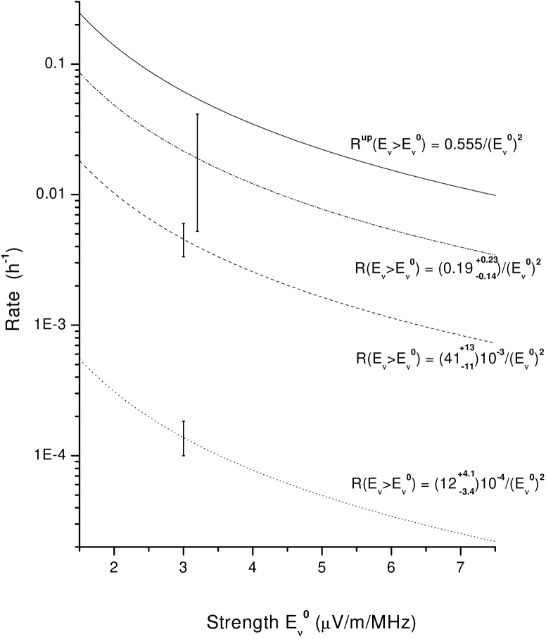
Divided by the total run time (17.245 hours with EW antenna polarization and 21.116 hours with NS polarization), $N^{up}$ gives the upper limit on the rate of signal pulses of strength greater than ${\cal E}_{\nu}^{0}$. We will denote it $R^{up}({\cal E}_{\nu}>{\cal E}_{\nu}^{0})$. Of course, one can obtain different values of $R^{up}({\cal E}_{\nu}>{\cal E}_{\nu}^{0})$ when looking for a different significant number of entries in the interesting bin. We searched for the accumulation values from 2 to 20 in the bin $(-7,-6)~{}\mu s$. The lowest $R^{up}({\cal E}_{\nu}>{\cal E}_{\nu}^{0})$ gives the most stringent upper limit on the rate. Its value also depends on criteria imposed on both signal and noise pulses. The best results were achieved when all three criteria (a), (b) and (c) were employed. The ratio threshold parameter for criterion (b) was tested in the region from 1 to 2.4 with step 0.2. The thresholds that give the best results were found to be 1.4 for EW and both 1.6 and 1.8 for NS data. Compared to the analysis with neither (b) nor (c) employed, these threshold parameters provide up to 28% lower upper limits. The resulting values of $R^{up}({\cal E}_{\nu}>{\cal E}_{\nu}^{0})$ are shown as dots in Fig. 15 for several values of ${\cal E}_{\nu}^{0}$ for the data taken with both East-West and North-South polarizations. Signal pulses stronger than 4.57 $\mu$V/m/MHz are expected to be quite rare and were definitely absent from the NS data, just like pulses stronger than 6.85 $\mu$V/m/MHz were absent from the EW data. Zero upper limits on the rates of these events are indicators of these facts.

Figure 15: Upper limit $R^{up}({\cal E}_{\nu}>{\cal E}_{\nu}^{0})$ on the rate of signal pulses stronger than a fixed strength ${\cal E}_{\nu}^{0}$. Plotted dots show the upper limit for antenna system gain $G=1.8$. Small numbers near the dots indicate $N^{up}$, the upper limit on the number of the signal events in the run. The dots were plotted for the pulses that are stronger than $1/n$ times the original test pulse amplitude of 13.7 $\mu$V/m/MHz, $n=2,3,\ldots,7$. The solid line represents the lowest upper limit corresponding to them. Data were taken with (a) North-South (21.12 hours) and (b) East-West (17.25 hours) antenna polarization.

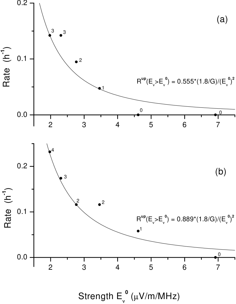
As was mentioned above, the differential rate $R({\cal E}_{\nu})$ should be proportional to $1/{\cal E}_{\nu}^{3}$. Then, the rate of signal pulses of the strength greater than ${\cal E}_{\nu}^{0}$ is

$$R({\cal E}_{\nu}>{\cal E}_{\nu}^{0})=\int\limits_{{\cal E}_{\nu}^{0}}^{+\infty}R({\cal E}_{\nu})\,d{\cal E}_{\nu}\propto\int\limits_{{\cal E}_{\nu}^{0}}^{+\infty}\frac{1}{{\cal E}_{\nu}^{3}}\,d{\cal E}_{\nu}\propto\frac{1}{({\cal E}_{\nu}^{0})^{2}}$$

i.e., proportional to $1/({\cal E}_{\nu}^{0})^{2}$. Hence, the lowest curve $c/({\cal E}_{\nu}^{0})^{2}$ passing through one of the nonzero dots (solid line in Fig. 15) represents the strictest upper limit on this rate. The value of the coefficient $c$ was found to be 0.555 for the NS data and 0.889 for the EW data:

$$R^{up}({\cal E}_{\nu NS}>{\cal E}_{\nu}^{0})=0.555/({\cal E}_{\nu}^{0})^{2}\ \ {\rm h}^{-1},$$ (2)

$$R^{up}({\cal E}_{\nu EW}>{\cal E}_{\nu}^{0})=0.889/({\cal E}_{\nu}^{0})^{2}\ \ {\rm h}^{-1},$$ (3)

where ${\cal E}_{\nu}^{0}$ is in $\mu$V/m/MHz. These results should be interpreted as the upper limits on the rates of events where the North-South (or East-West) projection of the signal pulse was greater than some value. We will use them in Appendix A for sensitivity calculations.

5.4 Discussion and summary

The small duration of the present subset of data prevents us from confirming or refuting previous claims for shower pulses. As mentioned, this subset was taken with CASA HV off, and was initially collected in order to check indications of a signal which occurred with CASA HV on. Using the estimate of 2.25 strong signal pulses per day [Sec. 4.4.4], one expects about three or four detectable shower pulses during 38.36 hours of observation. Three or four detectable particles that might give a strong signal during the experiment would be too scanty an amount to be detected over the noise background, which closely mimics genuine signals.

Figure 16: Rate of events at the CASA detection area in which the East-West projection of the signal pulse is greater than some ${\cal E}_{\nu}^{0}$. The lower three curves show the predicted rates based on different values of $s$: $s=20\pm 9.5$ (dash-dotted line, the original Haverah Park result [3] based on $\sim$100 detected shower pulses); $s=9.2\pm 1.4$ (dashed line, the Soviet group result [4] based on $\sim$1000 pulses), and $s=1.6\pm 0.24$ (dotted line, the updated Haverah Park result [4] based on $\sim$1000 pulses). The uncertainty in the latter two values is 15% [4]. We evaluated the uncertainty in the former as being $\sqrt{10}\cdot 15\%\approx 47\%$. In this logarithmic plot the error bars have constant lengths along their corresponding curves. The top curve is the upper limit in this paper which corresponds to $s=31$. These four curves are determined under the assumption of a transverse current radiation mechanism [10].

Figure 17: Rate of events at the CASA detection area in which the North-South projection of the signal pulse is greater than some ${\cal E}_{\nu}^{0}$. The lower three curves show the predicted rates based on different values of $s$: $s=20\pm 9.5$ (dash-dotted line, the original Haverah Park result [3] based on $\sim$100 detected shower pulses); $s=9.2\pm 1.4$ (dashed line, the Soviet group result [4] based on $\sim$1000 pulses), and $s=1.6\pm 0.24$ (dotted line, the updated Haverah Park result [4] based on $\sim$1000 pulses). The uncertainty in the latter two values is 15% [4]. We evaluated the uncertainty in the former as being $\sqrt{10}\cdot 15\%\approx 47\%$. In this logarithmic plot the error bars have constant lengths along their corresponding curves. The top curve is the upper limit in this paper which corresponds to $s=34$. These four curves are determined under the assumption of a particular radiation mechanism discussed in Appendix A.

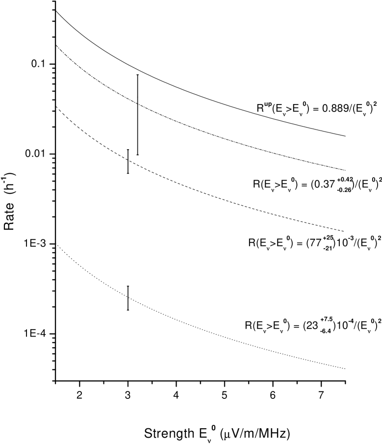
Nonetheless, we were able to place upper limits on the integral rate of signal pulses. Under certain simplifying assumptions these upper limits can be used for evaluating the numerical calibrating factor $s$. This factor was set to 20 in Eq. (1) but there remained an uncertainty regarding its value. In fact, subsequent reports claimed values as small as 1.6. We could only set upper limits on $s$: $s<31$ from the EW and $s<34$ from the NS data [see Appendix A]. The former was obtained under the assumption of the transverse current radiation mechanism, the latter under an alternative radiation mechanism discussed in Appendix A. Figs. 16 and 17 compare our results with those of previous experiments.

Had additional observation time with CASA boxes disabled been available, more signal pulses and more noise transients would be recorded. Would it be easier to prove the presence of shower signals in the data? Taking into account that the average signal pulse from a high energy air shower is much stronger than the average noise pulse, the content of the most intense transients (those stronger than 17th strongest, 39th, etc.) would shift in favor of more signal pulses. Thus, additional running time with CASA HV off would have allowed one to at least place a stricter upper limit on the rate of shower pulses, if not to detect them.

6 Issues specific to a giant array

6.1 Frequency range

The study of pulse components above 30 MHz remains a useful restriction in view of the changing RF environment encountered at lower frequencies. During years of sunspot minima the whole range of frequencies above 23 MHz remained relatively clear of broadcast interference, while as the sunspot numbers increased toward the end of 1997, daytime interference became particularly intense from the citizen’s band just above 27 MHz. This interference typically subsided at sunset. If observations below 30 MHz are contemplated, they would be most useful during years of expected sunspot minima (e.g., 2006-7), to minimize effects of long-distance ionospheric reflections.

6.2 Number and spacing of receiving sites

It is expected [3] that signals above 30 MHz decrease rapidly as a function of distance between the antenna and the shower core’s closest approach. Thus, we expect that in the Auger array, with spacing of 1.5 km between sites in a hexagonal array, RF stations would have to be distributed with roughly the same or greater density. One possibility for minimizing RF interference from Auger stations would be to place the RF station at the interstices between them. This would raise the cost per station, since it would require microwave communication with Auger sites and auxiliary sources of power.

At each station it may be helpful to have two antennas, one registering pulses of east-west polarization and one for north-south polarization. Differential signals as well as individual ones should be recorded. Coincidences among several stations may be associated with particularly large showers. Frequency-dependent antenna phase response should be modeled or measured, as noted in Sec. 4.4.8.

6.3 Digitization requirements

Previous work by one of us (J.F.W.) involved detection of electromagnetic pulses, including those possibly produced by cosmic-ray-induced electromagnetic discharges, with frequencies in the 30 – 100 MHz range. Part of this work included building hardware for self-triggering on short duration wide-band RF pulses. Many of the pulse identification, fast-digitization and memory problems were identical to those for pulse detection at CASA/MIA. Time-frequency plots were obtained similar to those one would generate in a survey at CASA/MIA. Similar requirements also are encountered for digitization of data from the KamLAND Experiment [38].

Our experience with the present system indicates the need for expanded dynamic range if continuous-wave sources of RF interference (such as FM and TV broadcast stations) are to be eliminated digitally. Thus, one needs at least 10-bit and probably 12-bit range, with a digitization rate of at least 400 MHz so as to be sensitive to frequencies up to 200 MHz. Although the expected signal is likely to be concentrated at lower frequencies (probably below 100 MHz), the expanded frequency range has proved useful in distinguishing expected signals from other transients.

6.4 Stand-alone trigger

Our results do not indicate that a trigger based on RF signals alone can yield useful correlations with air shower events. This result may be specific to the location of the CASA/MIA array; such a trigger may be less subject to noise at a remote location such as the Southern Hemisphere Auger site. An RF survey performed there would be useful in determining the utility of such a trigger. At such a site, more free from man-made noise than the CASA/MIA site, one would have to perform further studies allowing discrimination between random triggers (such as those induced by atmospheric discharges) and those induced by air showers. One would also attempt to detect galactic noise as a further indication that the site was sufficiently quiet.

6.5 Integration into the data stream

The data of CASA/MIA and that of the RF detection experiment were only integrated off-line. Any further studies should allow for simultaneous acquisition of both sets of data. Since the Auger project proposes to use microwave communication between stations, this same link should be considered for communicating RF signal acquisition results to a central data stream.

6.6 Status of GHz detection

David Wilkinson, who visited the University of Chicago during the spring of 1995, has proposed looking into the power radiated at frequencies of several GHz, where new opportunities exist associated with the availability of low-noise receivers. These techniques have now been implemented in the RICE project [39], which seeks to detect pulses with frequency components around 250 MHz in Antarctic polar ice.

6.7 Other options

Dispersion between arrival times of GPS signals on two different frequencies may serve as a useful monitor of air shower activity. The possibility of correlation of large showers with such dispersion events could be investigated.

It may be possible to monitor commercial broadcast signals in the 54 - 216 MHz range to detect momentary enhancements associated with large showers, in the same sense that meteor showers produce such enhancements. Television channels for which no nearby stations exist offer one possibility. The data taken at CASA/MIA have not yet been analyzed in terms of such enhancements, but represent a potential source of information. In Table 11 we note the locations of TV stations broadcasting on VHF channels other than those assigned to the Salt Lake City metropolitan area within 400 km of Dugway. These are channels 3 (60–66 MHz), 6 (82–88 MHz), 8 (180–186 MHz), 10 (192-198 MHz), and 12 (204-210 MHz). The availability of at least two stations on Channel 3 and three on Channel 6 at greatly differing headings indicates that this method may have some promise.

Table 11: Television stations within 400 km of Dugway on channels not assigned to the Salt Lake City metropolitan area. Ref. [26] also lists four “new” (unidentified) stations on Channel 3 for Price, UT (distance $\simeq$ 160 km, heading $\simeq$ 110 degrees) and two on Channel 12 for Logan, UT (distance 178 km, heading 14 degrees).

Call	Location	Channel	Power	Distance from	Heading
sign			(kW)	Dugway (km)	(degrees)
KBJN	Ely, NV	3	100	212	239
KIDK	Idaho Falls, ID	3	100	363	1
KBNY	Ely, NV	6	100	212	239
KPVI	Pocatello, ID	6	100	301	6
KBCJ	Vernal, UT	6	83.2	306	87
KIFI-TV	Idaho Falls, ID	8	316	363	1
KENV	Elko, NV	10	3.09	272	280
KISU-TV	Pocatello, ID	10	123	301	6
KUSG	St. George, UT	12	10	359	191

Radar detection of showers offers another exciting possibility [19]. This method resembles the use of distant fixed VHF stations for generating reflections off showers, but allows for a more carefully controlled environment.

7 Conclusions

A prototype system for the detection of radio-frequency (RF) pulses associated with extensive air showers of cosmic rays was tested at the Chicago Air Shower Array and Michigan Muon Array (CASA/MIA) in Dugway, Utah. This system was under consideration for use in conjunction with the Pierre Auger Project, which seeks to study showers with energies above $10^{19}$ eV.

The system utilized a trigger based on the coincidence of 7 out of 8 buried muon detectors around the periphery of the CASA array. Transients were indeed detected in conjunction with large showers, but they were identified as arising from the CASA modules themselves, most likely from the electronics generating trigger request (TRQ) pulses. Such transients could be eliminated when the high voltage (HV) on CASA phototubes was turned off; in such cases the muon trigger continued to function. By comparing upper limits on detected transients with simulated pulses, it was possible to place upper bounds on the rate of detection of RF pulses of various intensities. These upper bounds are summarized in Fig. 15; they typically involve rates of one every few hours for the largest field strengths claimed in the literature [4]. Based on our estimates, it is unlikely that the present experiment can reach the sensitivity limits of the Haverah Park results, which reported lower field strengths in their latest work [4].

A number of lessons have been learned from the present exercise. These are probably most relevant for any installation contemplated in conjunction with the proposed Auger project [14].

(1) One must take special care to survey transients produced by components of the array. For the Auger detector, one must install one or more antennae close to the proposed Čerenkov detectors and their associated digitizers, and study the response to artificially induced signals. Based on our experience, in which the present bounds are based on a small subset (38 hours) of the total data sample (600 hours), one should focus as soon as possible on a configuration in which usable data can be gathered.

(2) The method of communication between Auger modules will affect what form of RF detection is feasible. If radio links employing microwave ($>800$ MHz) frequencies are used, the present system will not be as seriously compromised as it apparently was by the communication system used at CASA/MIA. On the other hand, detection of RF signals above 1 GHz will suffer interference from such a system.

(3) Consideration should be given to placement of antennas at sites sufficiently far from surface detector modules that pulses from these modules do not constitute a serious source of interference. In the Auger case, the modules are arranged in a triangular array with 1.5 km spacing, so that the maximum spacing between an antenna inside the array and any module could be as large as $1.5/\sqrt{3}\simeq 0.87$ km if the antenna is placed at an equal distance from the three closest modules.

(4) Coincidence between RF signals detected at several antennas is desirable, as was found in the earliest experiments [2].

(5) The digital filtering algorithms employed in the present study, although not yet pushed to their optimal efficiencies, appear to be limited by the 8-bit dynamic range employed in detection using a digitizing oscilloscope. Consideration should be given to a system with larger dynamic range, at least 10-bit but preferably 12-bit.

(6) One can probably afford to economize by reducing the sampling rate, certainly to 500 MSa/s but perhaps as low as 200 MSa/s, since transients are expected to have their main frequency components below 100 MHz, and by reducing the active sampling window from the present value of 50 $\mu$s to a lower value, depending on the geometry of the array.

(7) The frequency range studied in the present work (23–200 MHz) will be more useful if continuous RF sources, such as FM and television stations, are much weaker than they were at the Dugway site. This is a possibility in the remote Argentine site at which the first Auger array is to be constructed [14]; a survey of field strengths there would be desirable.

(8) One should take data simultaneously with two antennas polarized in perpendicular (EW and NS) directions. This allows the determination of two components of the electric vector, not just one of its projections.

Although no RF signals have been detected in conjunction with CASA/MIA events, the present study has revealed a number of useful criteria for future experiments of similar type. It is hoped that a prototype at an Auger site will further focus these criteria.

Appendix A: Sensitivity Calculation

One of the aims of this study was to evaluate the antenna response as a function of shower parameters. The dependence on $R$, $\theta$, $\alpha$, $E_{p}$ has been established in [3] (Eq. (1)). However, there remained an uncertainty as regards the calibrating factor $s$, for which experimental data do not supply an exact value. Indeed, we have quoted at least three versions of it: first, in Eq. (1) it is set to 20; second, the Haverah Park group subsequently reported that ${\cal E}_{\nu}^{N}=0.6$, while the Soviet group claimed the value of 3.4 [4]. To make the connection between ${\cal E}_{\nu}^{N}$ and $s$, let us note that $s\simeq{\cal E}_{\nu}^{N}/\exp(-1)$. Thus, we can infer that the Haverah Park group updated Eq. (1) to $s=1.6$, and the Soviet group to $s=9.2$.

Ideally, we would like to calculate the calibrating factor precisely from the rate $R({\cal E}_{\nu EW}>{\cal E}_{\nu}^{0})$, but unfortunately this rate cannot be obtained accurately from experiment; we could only set an upper bound on it (Section 5.3.4). Hence, in this Appendix we will be able to set only an upper limit on $s$ to get at least some evaluation of the possible range of its values. We will do it in the following way.

Equation (1) and the exact knowledge of the coefficient $k$ in the formula for the rate of primaries as a function of their energy $R(E_{p})=k/E_{p}^{3}$ [29] can be used to calculate the rate $R({\cal E}_{\nu EW}>{\cal E}_{\nu}^{0})$. The result will certainly depend on the calibrating factor $s$. Comparing this rate with the experimental upper bound, $R^{up}({\cal E}_{\nu EW}>{\cal E}_{\nu}^{0})$, an upper limit will be placed on the calibrating factor.

In the process of evaluating $R({\cal E}_{\nu EW}>{\cal E}_{\nu}^{0})$ we will need to integrate the rate of primaries $R(E_{p})$ over solid angle, energy, and detection area. The question of detection area is of great importance since its lack of symmetry with respect to the antenna compelled us to make an important simplifying assumption.

Detection area

Figure 18: Core locations for 1702 showers giving rise to muon triggering. The opening angle at the antenna vertex is 2 radians. The radii of the inner and outer circular arcs are 100 and 400 m, respectively. Axes relative to center of array are $x$ (geographic East) and $y$ (geographic North), in meters.

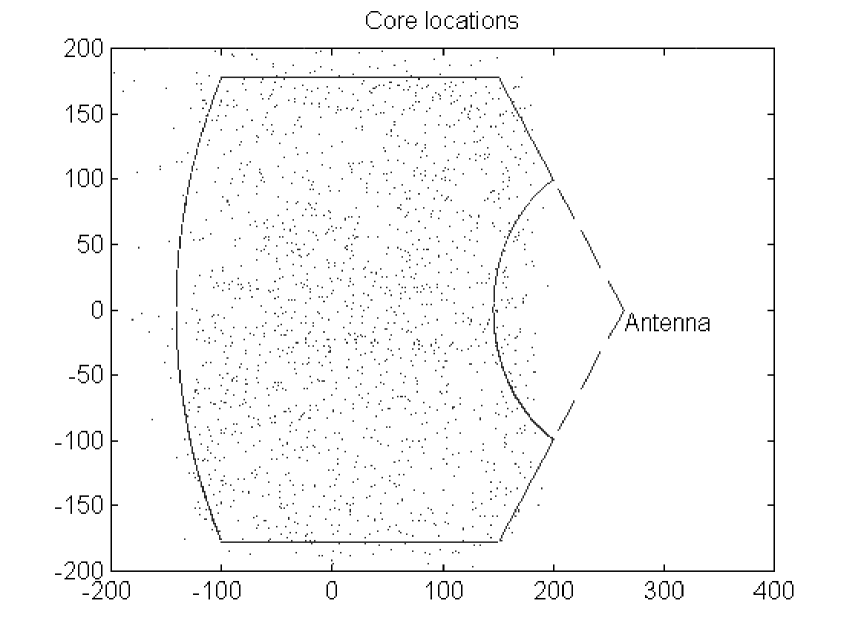
Core locations of showers that fire muon triggering are shown in Fig. 18. Their distribution over the outlined area appears to be approximately uniform. To simplify the integration over solid angle, area, and energy, let us consider a bigger area: part of the ring with inner radius of 100 m, outer radius of 400 m, inside the same angle of 2 radians. The rate of showers passing through this area is bigger than through the one shown in Fig. 18. Integration over the bigger area will lead to a greater value for $R({\cal E}_{\nu EW}>{\cal E}_{\nu}^{0})$. However, that value will differ from the one calculated after integration over the outlined area by less than 5%, as we show below in Calculation.

As was mentioned in Section 4.6, systematic studies have been performed only for simulated pulses with $\delta=5$ ns. Thus, $R^{up}({\cal E}_{\nu EW}>{\cal E}_{\nu}^{0})$ [Fig. 15(b)] was obtained under the assumption $R\simeq 200$ m. Though in reality the detection area is not limited to the area around 200 m, we are going to accept that result as a reasonable approximation.

Unfortunately, the area under consideration is not the full ring. If it were, it could have been proven that the angular distribution of the electric vector in the horizontal plane is approximately uniform. Then it would have been easy to derive $R({\cal E}_{\nu EW}>{\cal E}_{\nu}^{0})$ after calculating $R({\cal E}_{\nu}>{\cal E}_{\nu}^{0})$. In that case we wouldn’t have to worry about the polarization of radiation from individual showers.

In our case, however, the area is not symmetric. The general approach of calculating ${\cal E}_{\nu EW}$ for showers with different zenith angles, azimuth angles and core locations and then integrating would be too difficult to implement. Therefore, it would be reasonable to simplify the problem by making the assumption that all showers are vertical. This will lead to a rough estimate of the upper limit that can be placed on the calibrating factor.

Now we are almost ready to perform integration. Only one thing is missing: Since $R^{up}({\cal E}_{\nu EW}>{\cal E}_{\nu}^{0})$ was calculated for the EW projection of the electric field vector, we will need a relation between ${\cal E}_{\nu}$ and ${\cal E}_{\nu EW}$ for showers with different core locations. For this purpose let us turn to the question of polarization of radiation produced by a shower.

Polarization

The conventional approach assumes linear polarization in the direction perpendicular to both shower axis and magnetic field vector. The source of such radiation is the transverse current of shower particles [10]. Alternatively, one can consider radio emission due to particles’ acceleration in the Earth’s magnetic field. For the time being we will pursue the latter approach but at the end of this Appendix we will give results for both alternatives.

The magnitude and direction of the electric field vector for a radiating particle are governed by the general formula

$${\bf E}({\bf x},t)=e\,\left[\frac{{\bf n}-\boldsymbol{\beta}}{\gamma^{2}(1-\boldsymbol{\beta}\cdot{\bf n})^{3}\,l^{2}}\right]_{\rm ret}+\frac{e}{c}\,\left[\frac{{\bf n}\times\left[({\bf n}-\boldsymbol{\beta})\times\dot{\boldsymbol{\beta}}\right]}{(1-\boldsymbol{\beta}\cdot{\bf n})^{3}\,l}\right]_{\rm ret}\ \ \ \ \ \ \ (A.1)$$

where $\boldsymbol{\beta}$ is the velocity vector in the units of $c$, $\dot{\boldsymbol{\beta}}=d\boldsymbol{\beta}/dt$ is the acceleration vector, divided by $c$, ${\bf n}$ is a unit vector from the radiating particle to the antenna, and $l$ is the distance to the particle [40]. The square brackets with subscript “ret” mean that the quantities in the brackets are evaluated at the retarded time. (A.1) does not consider the influence of the index of refraction of air. Here we are primarily interested in the direction of the electric field vector and for $R>100$ m the effect of the refraction index on polarization is insignificant. Ref. [36] will give a full calculation of shower radiation, employing a modified formula (A.1) to take into account the refraction index.

The first term in (A.1) decreases with distance as $1/l^{2}$ and represents a boosted Coulomb field. It does not produce any radiation. The magnitudes of two terms in (A.1) are related as $1/(\gamma^{2}l)$ and $|\dot{\boldsymbol{\beta}}|/c$. The characteristic acceleration of a 30 MeV electron ($\gamma\approx 60$) of an air shower in the Earth’s magnetic field ($B\approx 0.5$ Gauss) is $|{\bf a}|=ecB/(\gamma m)\approx 4.4\cdot 10^{13}$ m/s². Even when an electron is as close to the antenna as 1000 m, the first term is three orders of magnitude smaller than the second and can be neglected. The second term falls as $1/l$ and is associated with a radiation field. It describes the electric field of a single radiating particle for most geometries relevant to extensive air showers.

Figure 19: Geometry of a vertical shower. Axes relative to antenna are $x$ (magnetic West), $y$ (magnetic South) and $z$ (up). Vector B lies in the $yOz$ plane.

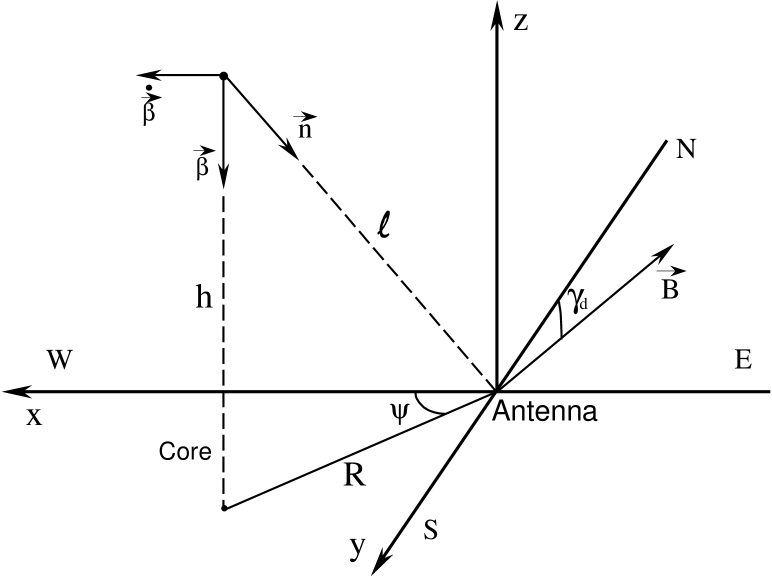
Consider the frame centered at the antenna, with axis $Ox$ going to the magnetic West, $Oy$ to the South and $Oz$ directly up. For vertical showers in this frame $\boldsymbol{\beta}=(0,0,-1)$, while $\dot{\boldsymbol{\beta}}$ is parallel to $Ox$, or, in other words, to the $(1,0,0)$ vector (see Fig. 19).  Let $\psi$ be the angle between $Ox$ and the direction to the shower core, $R$ the distance to the core, and $h$ the altitude of the radiating particle. Then ${\bf n}=\left(-\frac{R\cos\psi}{\sqrt{h^{2}+R^{2}}},-\frac{R\sin\psi}{\sqrt{h^{2}+R^{2}}},-\frac{h}{\sqrt{h^{2}+R^{2}}}\right)$. Typical values for $R$ are a few hundred meters, and for $h$ several kilometers, so $R/h$ can be considered small. The denominator of the second term of Eq. (A.1) is independent of $\psi$. The numerator determines that, to leading (second) order in $R/h$, the electric field vector lies in the horizontal plane and is parallel to $(\cos 2\psi,\sin 2\psi,0)$. The magnitude of the numerator is independent of the angle $\psi$ up to terms of the order $R^{4}/h^{4}$.

This result shows that although particles are accelerated by the Earth’s magnetic field in the EW direction, the polarization of the resulting radiation does not show preference for a particular direction. In other words, assuming uniform distribution of shower cores around the antenna (uniform distribution of $\psi$), one obtains a uniform angular distribution of the electric field vector.

The most important result of this section for the following calculation is the relation between ${\cal E}_{\nu EW}$ and ${\cal E}_{\nu}$:

$${\cal E}_{\nu EW}={\cal E}_{\nu}|\cos 2\psi|$$

Calculation

Let us now calculate the rate $R({\cal E}_{\nu EW}>{\cal E}_{\nu}^{0})$ as a function of $s$. For vertical showers Eq. (1) becomes

$${\cal E}_{\nu}=s\,\frac{E_{p}}{10^{17}~{}\mbox{eV}}\,\cos\gamma_{d}\,\exp\left(-\frac{R}{R_{0}(\nu,0)}\right)\ \ \ \ \mu\mbox{V m}^{-1}\mbox{MHz}^{-1}\,$$

where $s$ is the calibrating factor, and $\gamma_{d}$ is a dip angle (the angle between the magnetic field vector and the direction to magnetic North). $R_{0}(\nu,\theta)$ only depends slightly on $\theta$ when $\theta<35^{\circ}$. The dependence on $\nu$ is not very significant, either. Ref. [2] quotes two numbers: At $\nu=55$ MHz $R_{0}$ equals 110 m, while at $\nu=32$ MHz $R_{0}$ equals 140 m. The form of the dependence is not well known, although it is clear that $R_{0}$ becomes larger as $\nu$ decreases. Assuming linear dependence for simplicity, one can evaluate $R_{0}=130$ m at $\nu=39$ MHz, the median frequency of the main region of investigation [Section 5.3.1 (b)]. This value of $R_{0}$ will be used in this Appendix.

Consider showers with impact parameter $R$, direction to the core given by angle $\psi$, and primary energy

$$E_{p}>E^{\prime}_{p}({\cal E}_{\nu}^{0},R,\psi)={\cal E}_{\nu}^{0}\,\frac{10^{17}}{s\cos\gamma_{d}}\,\frac{\exp(R/R_{0})}{|\cos 2\psi|}\ \ \ \mbox{eV}$$

where ${\cal E}_{\nu}^{0}$ is expressed in $\mu\mbox{V m}^{-1}\mbox{MHz}^{-1}$. Only these showers induce ${\cal E}_{\nu EW}={\cal E}_{\nu}\,|\cos 2\psi|>{\cal E}_{\nu}^{0}$. So, the rate of events where the East-West projection of the pulse is greater than some value, $R({\cal E}_{\nu EW}>{\cal E}_{\nu}^{0})$, equals the rate $Z$ of such showers passing through the detection area.

Now let us determine the limits of integration. We assume that although we consider vertical showers only, the solid angle of observation is limited by a zenith angle $\theta_{m}=50^{\circ}$.

We also take into account that magnetic North at Dugway is located $14^{\circ}$ east of true North. Therefore, the detection area is bound by lines $\psi=57^{\circ}+14^{\circ}=71^{\circ}$ and $\psi=-57^{\circ}+14^{\circ}=-43^{\circ}$.

We know that the rate of primaries (in $\mbox{eV}^{-1}\mbox{km}^{-2}\mbox{sr}^{-1}\mbox{h}^{-1}$) is given by $R(E_{p})=k/E_{p}^{3}$. Hence, the integration over solid angle, area and energy gives the desired rate $Z$ (in $\mbox{h}^{-1}$)

$$\begin{array}[]{l}Z=\int d\Omega\int dA\int\limits_{E^{\prime}_{p}({\cal E}_{\nu}^{0},R,\psi)}^{+\infty}R(E_{p})\,dE_{p}=\\ \quad 2\pi\int\limits_{0}^{\theta_{m}}\sin\theta\,d\theta\int\limits_{-43^{\circ}}^{71^{\circ}}d\psi\int\limits_{100~{}\mbox{m}}^{400~{}\mbox{m}}R\,dR\int\limits_{E^{\prime}_{p}({\cal E}_{\nu}^{0},R,\psi)}^{+\infty}\frac{k}{E_{p}^{3}}\,dE_{p}=\\ \quad 2\pi(1-\cos\theta_{m})\int\limits_{-43^{\circ}}^{71^{\circ}}d\psi\int\limits_{100~{}\mbox{m}}^{400~{}\mbox{m}}R\,dR\,\,\frac{k}{2E_{p}^{\prime 2}}=\\ \quad\ \pi k(1-\cos\theta_{m})\left(\frac{s\cos\gamma_{d}}{10^{17}{\cal E}_{\nu}^{0}}\right)^{2}\int\limits_{-43^{\circ}}^{71^{\circ}}\cos^{2}2\psi\,d\psi\int\limits_{100~{}\mbox{m}}^{400~{}\mbox{m}}Re^{-2R/R_{0}}\,dR\ \ \ \ \ \ \ (A.2)\end{array}$$

Both integrals in Eq. (A.2) can be readily calculated to obtain the following expression:

$$R({\cal E}_{\nu EW}>{\cal E}_{\nu}^{0})=Z\approx\pi k(1-\cos\theta_{m})\left(\frac{s\cos\gamma_{d}}{10^{17}{\cal E}_{\nu}^{0}}\right)^{2}\cdot 2.0\cdot 10^{3}\ \ \ \ \ \mbox{h}^{-1}$$

where $k$ is in $\mbox{eV}^{2}\mbox{m}^{-2}\mbox{sr}^{-1}\mbox{h}^{-1}$ and ${\cal E}_{\nu}^{0}$ is in $\mu\mbox{V/m/MHz}$. Let us note here that integration over the area outlined in Fig. 18 (instead of the part of the ring) has also been calculated numerically with the help of Mathematica, with the result

$$R({\cal E}_{\nu EW}>{\cal E}_{\nu}^{0})\approx\pi k(1-\cos\theta_{m})\left(\frac{s\cos\gamma_{d}}{10^{17}{\cal E}_{\nu}^{0}}\right)^{2}\cdot 1.9\cdot 10^{3}\ \ \ \ \ \mbox{h}^{-1}$$

i.e., only a 5% difference. Thus, the rapidly decreasing exponential suppresses the contribution at large distances from the antenna where the part of the ring does not overlap the outlined area.

Now we can place an upper limit on $s$ using this formula for the rate $R({\cal E}_{\nu EW}>{\cal E}_{\nu}^{0})$ and the experimental upper limit on this rate, $R^{up}({\cal E}_{\nu EW}>{\cal E}_{\nu}^{0})$ from Section 5.3.4:

$$R({\cal E}_{\nu EW}>{\cal E}_{\nu}^{0})\approx\pi k(1-\cos\theta_{m})\left(\frac{s\cos\gamma_{d}}{10^{17}{\cal E}_{\nu}^{0}}\right)^{2}\cdot 1.9\cdot 10^{3}<R^{up}({\cal E}_{\nu EW}>{\cal E}_{\nu}^{0})\ \ \ \ \ (A.3)$$

$$s<\frac{10^{17}{\cal E}_{\nu}^{0}}{\cos\gamma_{d}}\cdot\sqrt{\frac{R^{up}({\cal E}_{\nu EW}>{\cal E}_{\nu}^{0})}{\pi k(1-\cos\theta_{m})\cdot 1.9\cdot 10^{3}}}\ \ \ \ \ \ \ \ \ \ \ \ (A.4)$$

¿From Eq. (3), ${\cal E}_{\nu}^{0}\cdot\sqrt{R^{up}({\cal E}_{\nu EW}>{\cal E}_{\nu}^{0})}\approx 0.943~{}\mu\mbox{V/m/MHz/h}^{1/2}$. This value, substituted into (A.4) together with $k=3.84\cdot 10^{24}~{}\mbox{eV}^{2}\mbox{m}^{-2}\mbox{sr}^{-1}\mbox{s}^{-1}=1.38\cdot 10^{28}~{}\mbox{eV}^{2}\mbox{m}^{-2}\mbox{sr}^{-1}\mbox{h}^{-1}\$ [29], $\theta_{m}=50^{\circ}$ and $\gamma_{d}=68^{\circ}$, gives the final result: $s<46$. A similar calculation employing North-South results [Eq. (2)] gives $s<34$.

If the main source of radiation is transverse current, not particles’ acceleration, then ${\bf E}$ is parallel to $\boldsymbol{\beta}\times{\bf B}$ [10] and for vertical showers ${\cal E}_{\nu EW}={\cal E}_{\nu}$. This changes the integral of $\cos^{2}2\psi$ over $\psi$ in formula (A.2) to the integral of 1 over $\psi$, leading to $s<31$. This is the smallest upper limit we can place on $s$. Unfortunately, this upper limit is not quite small enough to rule out the initial Haverah Park group claim of $s=20$, let alone the values of 9.2 or 1.6. To facilitate comparison of results of different studies, let’s rewrite formula (A.3) under the assumption of the transverse current mechanism. In simplified form it is

$$R({\cal E}_{\nu EW}>{\cal E}_{\nu}^{0})\approx 9.16\cdot 10^{-4}\,\left(\frac{s}{{\cal E}_{\nu}^{0}}\right)^{2}$$

The transverse current mechanism cannot account for the NS component for vertical showers so we will employ the model discussed above in Polarization. According to it, ${\cal E}_{\nu NS}={\cal E}_{\nu}|\sin 2\psi|$. Then, formula (A.3) transforms into

$$R({\cal E}_{\nu NS}>{\cal E}_{\nu}^{0})\approx 4.86\cdot 10^{-4}\,\left(\frac{s}{{\cal E}_{\nu}^{0}}\right)^{2}$$

The plots of $R({\cal E}_{\nu EW}>{\cal E}_{\nu}^{0})$ and $R({\cal E}_{\nu NS}>{\cal E}_{\nu}^{0})$ for different values of $s$ are shown in Figs. 16 and 17.

The noise level at Dugway is too high and the acquired sample is too limited in statistics and dynamic range to allow us to place upper limits strict enough to check the claims of the two groups. We hope that further improvement of the data processing technique will reduce the noise contribution. The dip angle $\gamma_{d}$ is much smaller at the Auger site in Argentina ($34^{\circ}$ versus $68^{\circ}$ at Utah). This leads to bigger electric fields for vertical showers, facilitating the detection of shower radiation. We also expect that the Argentina site will be quieter than Dugway and some clarity as regards the calibrating factor will be established.

Appendix B: Relation between simulated pulse strength and peak detected voltage

Within the bandwidth $\delta\nu$, the antenna feels the electric field ${\cal E}_{\nu}\cdot\delta\nu$. Then, the instantaneous power flow is given by $({\cal E}_{\nu}\cdot\delta\nu)^{2}/(120\pi)$, where $120\pi~{}\Omega$ is the impedance of free space. The antenna effective aperture is equal to $G_{ant}\,(\lambda^{2}/4\pi)$, $G_{ant}\simeq 2.5$ being the antenna gain. Hence, it supplies a power of

$$W=\frac{({\cal E}_{\nu}\cdot\delta\nu)^{2}}{(120\pi)}\cdot G_{ant}\,\frac{\lambda^{2}}{4\pi}$$

to the input of the feedline cable. Subsequently, this power is transmitted by 60 feet of RG-58U cable with average attenuation at 39 MHz estimated to be 1.44 dB or a factor of $L\simeq 1.4$ in power. So, the power at the input of the preamplifier is $W/L$. The impedances in the antenna system were matched, in particular, the resistance of the preamplifier was equal to the characteristic impedance of the cable, $R=50~{}\Omega$. The power at the input of the preamplifier is transformed into a peak voltage $V_{pk}$ across the preamplifier resistance $R$, i.e. $W/L=V_{pk}^{2}/R$. Thus,

$${\cal E}_{\nu}=\frac{1}{\delta\nu}\sqrt{W\,\frac{480\pi^{2}}{G_{ant}\lambda^{2}}}=\frac{\nu}{\delta\nu}\,\frac{2V_{pk}}{c}\,\sqrt{\frac{120\pi^{2}L}{G_{ant}R}}=\frac{\nu}{\delta\nu}\,\frac{2V_{pk}}{c}\,\sqrt{\frac{120\pi^{2}}{GR}}$$

where $G=G_{ant}/L\simeq 1.8$ is the antenna-cable system gain. For specific values used in data analysis (Sec. 5.3.1.) $\delta\nu=54-24=30$ MHz, $\nu=39$ MHz,

$${\cal E}_{\nu}=0.042\,\frac{V_{pk}}{\sqrt{G}}=0.031\,\frac{V_{pk}}{\sqrt{G/1.8}}\ \ \ \mu\mbox{V/m/MHz}$$

where $V_{pk}$ is in $\mu$V.

The above derivation implies that the electric field perceived by the antenna is due to frequencies in the $\delta\nu$ range only. However, the simulated pulse voltage with $V_{pk}=1.3$ mV has components in the whole frequency range (see Fig. 4, bottom), i.e., it is the result of an imaginary “electric field” with very diverse frequencies. To find what $V_{pk}$ would be if our antenna were sensitive to 24-54 MHz only, the forward and then inverse (for 24-54 MHz region) Fourier transforms of the simulated pulse voltage have been performed. The contribution of 24-54 MHz region into the pulse peak voltage of 1.3 mV appeared to be equal to 442 $\mu$V. This leads to a corrected formula:

$${\cal E}_{\nu}=0.031\,\frac{442}{1300}\,\frac{V_{pk}}{\sqrt{G/1.8}}=0.011\,\frac{V_{pk}}{\sqrt{G/1.8}}\ \ \ \mu\mbox{V/m/MHz}$$

This formula establishes the relation between the simulated pulse strength ${\cal E}_{\nu}$ and its peak voltage $V_{pk}$ at the filter-preamplifier configuration. $G=1.8$ was assumed throughout the paper.

Appendix C: Cost considerations for Auger project

At present we can only present a rough sketch of criteria for detection in the 30–100 MHz range. Data would be digitized at a 500 MHz rate at each station and stored in a rolling manner, with at least 20 microseconds of data in the pipeline at any moment. Upon receipt of a trigger signaling the presence of a “large” shower ($>10^{18}$ eV), these data would be merged into the rest of the data stream at each station.

Per station, we estimate the following additional costs, in US dollars, for RF pulse detection:

Two antennas and protection circuitry:	200	(a)
Mounting hardware:	100	(b)
Cables and connectors:	200	(c)
Preamps:	500	(d)
Digitization and memory electronics:	2000	(e)
Total per station:	3000	(f)

(a) Two military-surplus log-periodic antennas; crossed polarizations.

(b) Highly dependent on other installations at site. Antennas are to be pointed vertically but optimum elevation not yet determined.

(c) Antennas are mounted near central data acquisition site of each station, but sufficiently far from any sources of RF interference such as switching power supplies. Alternative location of receiving stations at interstitial positions in the array would require microwave communication links and auxiliary power supplies and would add to cost.

(d) Commercial GaAsFET preamps and gas discharge tubes.

(e) Subject to prototype development experience. Power requirements not yet known.

(f) The number of stations to be equipped with RF detection will depend on further prototype experience.

The above estimate assumes that one can power the preamps and DAQ electronics from the supply at each station without substantial added cost. It also assumes that a “large-event trigger” will be available at each station. One consideration may be the acquisition of antennas robust enough to withstand extreme weather (particularly wind) conditions.

For detection at frequencies above or below 30–100 MHz, the criteria are not yet well enough developed to permit any cost estimate.

References

- [1] J. V. Jelley et al., Nature 205, 327 (1965); Nuovo Cimento A46, 649 (1966); N. A. Porter et al., Phys. Lett. 19, 415 (1965); T. Weekes, in Radio Detection of High Energy Particles (Proceedings of First International Workshop RADHEP 2000, Los Angeles, California, 16–18 November 2000), AIP Conference Proceedings. No. 579, edited by D. Saltzberg and P. Gorham (AIP, Melville, NY, 2001), p. 3.
- [2] P. R. Barker, W. E. Hazen, and A. Z. Hendel, Phys. Rev. Lett. 18, 51 (1967); W. E. Hazen, et al., ibid. 22, 35 (1969); 24, 476 (1970).
- [3] H. R. Allan, in Progress in Elementary Particles and Cosmic Ray Physics, v. 10, edited by J. G. Wilson and S. G. Wouthuysen (North-Holland, Amsterdam, 1971), p. 171, and references therein.
- [4] V. B. Atrashkevich et al., Yad. Fiz. 28, 366 (1978).
- [5] K. Kadota et al., Proc. 23rd International Conference on Cosmic Rays (ICRC-23), Calgary, 1993, v. 4, p. 262; Tokyo Workshop on Techniques for the Study of Extremely High Energy Cosmic Rays, Tanashi, Tokyo, 27 – 30 Sept. 1993.
- [6] C. Castagnoli et al., Proc. ICRC-23, Calgary, 1993, v. 4, p. 258.
- [7] P. I. Golubnichii, A. D. Filonenko, and V. I. Yakovlev, Izv. Akad. Nauk 58, 45 (1994).
- [8] R. Baishya et al., Proc. ICRC-23, Calgary, 1993, V. 4, p. 266; Gauhati University Collaboration, P. Datta et al., Proceedings of RADHEP 2000 [1], p. 98.
- [9] G. A. Askar’yan, Zh. Eksp. Teor. Fiz. 41, 616 (1961) [Sov. Phys.–JETP 14, 441 (1962)]; Zh. Eksp. Teor. Fiz. 48, 988 (1965) [Sov. Phys.–JETP 21, 658 (1965)].
- [10] F. D. Kahn and I. Lerche, Proc. Roy. Soc. A 289, 206 (1966).
- [11] S. A. Colgate, J. Geophys. Res. 72, 4869 (1972).
- [12] R. R. Wilson, Phys. Rev. 108, 155 (1967).
- [13] R. A. Roussel-Dupré, A. V. Gurevitch, T. Tunnell, and G. M. Milikh, Los Alamos National Laboratory report LA-12601-MS, November, 1993.
- [14] Auger Collaboration, Pierre Auger Project Design Report (2nd Edition, November, 1996, revised March 14, 1997), Fermilab, 1997 (unpublished); J. W. Cronin, Rev. Mod. Phys. 71, S165 (1999).
- [15] J. L. Rosner and D. A. Suprun, Proceedings of RADHEP 2000 [1], p. 81, astro-ph/0101089.
- [16] E. Zas, F. Halzen, and T. Stanev, Phys. Rev. D 45, 362 (1992).
- [17] P. Gorham et al., Phys. Rev. E 62, 8590 (2000); D. Saltzberg et al., Phys. Rev. Lett. 86, 2802 (2001); D. Saltzberg et al., Proceedings of RADHEP 2000 [1], p. 225.
- [18] P. M. S. Blackett and A. C. B. Lovell, Proc. Roy. Soc. 177, 183 (1941).
- [19] P. W. Gorham, Astropart. Phys. 15, 177 (2001).
- [20] S. N. Vernov et al., Pis’ma v ZhETF 5, 157 (1967) [Sov. Phys.–JETP Letters 5, 126 (1967)]; Can. J. Phys. 46, S241 (1968).
- [21] A. Borione et al., Nucl. Instrum. Meth. A 346, 329 (1994).
- [22] D. A. Smith et al., J. Geophys. Res. 104, 4189 (1999).
- [23] L. F. Fortson et al., in Proceedings of the 26th International Conference on Cosmic Rays (ICRC 99), Salt Lake City, 17–25 August 1999, vol. 3, p. 125; ibid., vol. 5, p. 332, 335; J. Fowler, Ph. D. Thesis, University of Chicago, 1999 (unpublished).
- [24] K. Boothby et al., Ap. J. 491, L35 (1997); D. B. Kieda and S. P. Swordy, in Proceedings of the 26th International Conference on Cosmic Rays (ICRC 99), Salt Lake City, 17–25 August 1999, vol. 3, p. 191; S. P. Swordy and D. B. Kieda, Astropart. Phys. 13, 137 (2000).
- [25] T. Abu-Zayyad et al., in Proceedings of the 26th International Conference on Cosmic Rays (ICRC 99), Salt Lake City, 17–25 August 1999, vol. 3, p. 260 and vol. 5, p. 365; T. Abu-Zayyad et al., Nucl. Instr. Meth. A 450, 253 (2000).
- [26] As listed on the Web site http://stations.triathlon.net/cgi-radio/.
- [27] Microwave Filter Company, Inc., 6743 East Kinne St., East Syracuse, NY 13057.
- [28] The magnetic declination (14∘ east of true north) and inclination ( N) are taken, respectively, from a USGS chart of the Dugway site and the map site http://geomag.usgs.gov/dod.html.
- [29] M. A. Lawrence, R. J. O. Reid, and A. A. Watson, J. Phys. G 17, 733 (1991).
- [30] R. Gall and K. D. Green, UMC-CASA note, Aug. 23, 1996 (unpublished).
- [31] P. Mooney, private communication of specifications from Dorne and Margolin.
- [32] See http://www.eznec.com for further information and a demonstration version.
- [33] K. Gross, private communication.
- [34] Wavelab, Stanford University. See http://www-stat.stanford.edu/wavelab/
- [35] D. F. Sullivan, Master’s Thesis, University of Chicago, 1999 (unpublished).
- [36] D. A. Suprun, P. W. Gorham, and J. L. Rosner, astro-ph/0211273.
- [37] G. J. Feldman and R. D. Cousins, Phys. Rev. D 57, 3873 (1998).
- [38] A. D. Marino (for the KamLAND Collaboration), “Waveform Digitization in the KamLAND Experiment,” in Nuclear Physics in the 21st century, INPC conference, Berkeley, CA, 30 July – 3 August, 2001, edited by E. Norman and G. Wozniak; KamLAND Collaboration, F. Beiseer et al., “Waveform digitization for KamLAND,”, Poster P58, in Proceedings of the 19th International Conference on Neutrino Physics and Astrophysics (Neutrino 2000), Sudbury, Canada, 16–21 Jun 2000, edited by J. Law, et al. (North-Holland, Amsterdam, 2001), Nucl. Phys. B Proc. Suppl. 91, 2001.
- [39] G. Frichter, D. W. McKay, and J. P. Ralston, Phys. Rev. D 53, 1684 (1996); RICE Collaboration, Proceedings of 25th International Cosmic Ray Conference, Durban, South Africa, 28 July - 8 August 1997, edited by M. S. Potgieter, B. C. Raubenheimer, and D. J. van der Walt (World Scientific, 1998), preprint astro-ph/9709223; D. Besson, in Proceedings of RADHEP 2000 [1], p. 157; S. Razzaque et al., preprint astro-ph/0112505 (unpublished); I. Kravchenko et al., preprint astro-ph/0112372 (unpublished).
- [40] J. D. Jackson, Classical Electrodynamics, 2nd edition (Wiley, 1975), p. 657.