Stability of Satellites Around Close-in Extrasolar Giant Planets

Abstract

We investigate the long-term dynamical stability of hypothetical moons orbiting extrasolar giant planets. Stellar tides brake a planet’s rotation and, together with tidal migration, act to remove satellites; this process limits the lifetimes of larger moons in extrasolar planetary systems. Because more massive satellites are removed more quickly than less massive ones, we are able to derive an upper mass limit for those satellites that might have survived to the present day. For example, we estimate that no primordial satellites with masses greater than $7\times 10^{-7}~{}\mathrm{M_{\oplus}}$ ($\sim 70~{}\mathrm{km}$ radius for $\rho=3~{}\mathrm{g~{}cm^{-3}}$) could have survived around the transiting planet HD209458b for the age of the system. No meaningful mass limits can be placed on moons orbiting Jovian planets more than $\sim 0.6~{}\mathrm{AU}$ from their parent stars. Earth-like moons of Jovian planets could exist for $5~{}\mathrm{Gyr}$ in systems where the stellar mass is greater than $0.15~{}\mathrm{M_{\odot}}$. Transits show the most promise for the discovery of extrasolar moons — we discuss prospects for satellite detection via transits using space-based photometric surveys and the limits on the planetary tidal dissipation factor $Q_{p}$ that a discovery would imply.

1 INTRODUCTION

Each of the giant planets in our solar system posesses a satellite system. Since the discovery of planets in other solar systems (Marcy et al., 2000b), the question of whether these extrasolar planets also have satellites has become relevant and addressible. Extrasolar planets cannot be observed directly with current technology, and observing moons around them poses an even greater technical challenge. However, high precision photometry of stars during transits of planets can detect extrasolar moons either by direct satellite transit or through perturbations in the timing of the planet transit (Sartoretti & Schneider, 1999). Using these techniques, Brown et al. (2001) placed upper limits of $1.2$ Earth radii ($~{}\mathrm{R_{\oplus}}$) and $3$ Earth masses ($~{}\mathrm{M_{\oplus}}$) on any satellites orbiting the transiting planet HD209458b based on the Hubble Space Telescope transit lightcurve.

The tidal bulge that a satellite induces on its parent planet perturbs the satellite’s orbit (e.g., Burns, 1986), causing migrations in semimajor axis that can lead to the loss of the satellite. For an isolated planet, satellite removal occurs either through increase in the satellite’s orbital semimajor axis until it escapes, or by inward spiral until it impacts the planet’s surface (Counselman, 1973). In the presence of the parent star, stellar-induced tidal friction slows the planet’s rotation, and the resulting planet-satellite tides cause the satellite to spiral inward towards the planet (Ward & Reid, 1973; Burns, 1973). This effect is especially important for a planet in close proximity to its star, and has been suggested as the reason for the lack of satellites around Mercury (Ward & Reid, 1973; Burns, 1973).

In this paper, we apply tidal theory and the results of numerical orbital integrations to the issue of satellites orbiting close-in extrasolar giant planets. We place limits on the masses of satellites that extrasolar planets may posess, discuss the implications these limits have for the detection of extrasolar satellites, and apply our results to the issue of Earth-like satellites orbiting extrasolar giant planets.

2 TIDAL THEORY AND METHODS

According to conventional tidal theory, the relative values of the planetary rotation rate, $\Omega_{p}$, and the orbital mean motion of the moon, $n_{m}$ (both in units of $\mathrm{radians}/\mathrm{sec}$), determine the direction of orbital evolution (see e.g., Murray & Dermott, 2000). For a moon orbiting a planet slower than the planet rotates ($n_{m}<\Omega_{p}$), the tidal bulge induced on the planet by the satellite will be dragged ahead of the satellite by an angle $\delta$, with $\tan(2\delta)=1/Q_{p}$. Here, $Q_{p}$ is the parameter describing tidal dissipation within the planet (after Goldreich & Soter, 1966), with $1/Q_{p}$ equal to the fraction of tidal energy dissipated during each tidal cycle. Gravitational interactions between the tidal bulge and the satellite induce torques that transfer angular momentum and dissipate energy, slowing the planet’s rotation and increasing the orbital semimajor axis of the satellite. Conversely, for satellites orbiting faster than their planet’s rotation ($n_{m}>\Omega_{p}$), the planet is spun up and the satellite’s semimajor axis decreases. The same mechanism causes torques on the planet from its parent star which slow the planet’s rotation (Murray & Dermott, 2000).

The torque on the planet due to the tidal bulge raised by the moon ($\tau_{p-m}$) is (Murray & Dermott, 2000)

$$\tau_{p-m}~{}=~{}-\frac{3}{2}\frac{k_{2p}~{}G~{}M_{m}^{2}~{}R_{p}^{5}}{Q_{p}~{}a_{m}^{6}}~{}\mathrm{sign}(\Omega_{p}-n_{m})~{}\mathrm{,}$$ (1)

where $k_{2p}$ is the tidal Love number of the planet, $R_{p}$ is the radius of the planet, and $G$ is the gravitational constant. The term $\mathrm{sign}(\Omega-n_{m})$ is equal to $1$ if $(\Omega-n_{m})$ is positive, and is equal to $-1$ if it is negative. We obtain the expression for the stellar torque on the planet by replacing $M_{m}$, the mass of the moon, with $M_{*}$, the mass of the star; by replacing $a_{m}$, the semimajor axis of the satellite’s orbit with $a_{p}$, the semimajor axis of the planet’s orbit about the star (circular orbits are assumed); and by using the planet’s mean orbital motion $n_{p}$ instead of $n_{m}$:

$$\tau_{p-*}~{}=~{}-\frac{3}{2}\frac{k_{2p}~{}G~{}M_{*}^{2}~{}R_{p}^{5}}{Q_{p}~{}a_{p}^{6}}~{}\mathrm{sign}(\Omega_{p}-n_{p})~{}\mathrm{.}$$ (2)

The moon’s semimajor axis, $a_{m}$, and the moon’s mean motion, $n_{m}$, are related by Kepler’s law, $n_{m}^{2}a_{P}^{3}=GM_{p}$. These torques affect both $n_{m}$ and $\Omega_{p}$. The rate of change of $\Omega_{p}$ is obtained by dividing the total torque on the planet by the planet’s moment of inertia:

$$\frac{d\Omega_{p}}{dt}~{}=~{}\frac{\tau_{p-m}+\tau_{p-*}}{I_{p}}~{}\mathrm{,}$$ (3)

where $I_{p}$ is the planet’s moment of inertia.

Under the circumstances studied in this paper, where a planet is orbited by a much smaller satellite, $\tau_{p-*}$ is much greater than $\tau_{p-m}$ for most of the system’s lifetime. Because the moon’s orbital moment of inertia depends on $n_{m}$, the equivalent expression for $n_{m}$ is less trivial to derive. We obtain it by setting the torque equal to the rate of change of the angular momentum and solving for $dn/dt$ using the planet’s mass, $M_{p}$ (e.g., Peale, 1988):

$$\frac{dn_{m}}{dt}~{}=~{}\frac{3~{}\tau_{p-m}~{}n_{m}^{4/3}}{M_{m}~{}(GM_{p})^{2/3}}~{}\mathrm{.}$$ (4)

Given appropriate initial and boundary conditions, integration of Equations 3 and 4 determines the state of the system at any given time.

An important boundary condition for such an integration is the critical semimajor axis, or the location of the outermost satellite orbit that remains bound to the planet. This location must be within the planet’s gravitational influence, or Hill sphere, and has been generally thought to lie between $1/3$ and $1/2$ the radius of the Hill sphere ($R_{H}$) (Burns, 1986), where

$$R_{H}=a_{p}\left(\frac{M_{p}}{3M_{*}}\right)^{1/3}~{}\mathrm{.}$$ (5)

Recently, Holman & Wiegert (1999) investigated the stability of planets in binary star systems and their results are applicable to the planet-satellite situation as well. Through numerical integrations of a test particle orbiting one component of a binary star system, Holman & Wiegert (1999) found that for high mass ratio binaries, the critical semimajor axis for objects orbiting the secondary in its orbital plane is equal to a constant fraction ($f$) of the secondary’s Hill radius, or

$$a_{crit}=fR_{H}~{}\mathrm{.}$$ (6)

We treat a star orbited by a much less massive planet as a high mass ratio binary system and deduce that the critical semimajor axis for a satellite orbiting the planet is $.36R_{H}$ ($f=.36$) for prograde satellites (from Holman & Wiegert, 1999, Figure 1). This agrees closely with Burns (1986). In fact, none of the prograde moons of our solar system orbit outside this radius (see Table 1). Holman & Wiegert (1999) did not treat objects in retrograde orbits (which are expected to be more stable than prograde ones), so to treat possible captured satellites we take $f_{retrograde}=0.50$ based on the solar system values for ${a_{m}}/{R_{H}}$ in Table 1.

3 CONSTRAINTS ON SATELLITE MASSES

Satellites orbiting close-in giant planets fall into one of three categories based on the history of their orbital evolution. Satellites that either start inside the planet’s synchronous radius (the distance from the planet where $n_{m}=\Omega_{p}$) or become subsynchronous early in their lifetimes, as a result of the slowing planetary rotation, spend their lives spiraling inward toward the cloud tops. Eventually these moons collide with the planet or are broken up once they migrate inside the Roche limit. Moons that start and remain exterior to the synchronous radius evolve outward over the course of their lives and, given enough time, would be lost to interplanetary space as a result of orbtial instability. In between these two is a third class of orbital history. In this case, a satellite starts well outside the synchronous radius and initially spirals outward, but its migration direction is reversed when the planet’s rotation slows enough to move the synchronous radius outside the moon’s orbit. These moons eventually impact the planet.

In order to determine which satellites might still exist around any given planet, we determine the maximum lifetime for a moon with a given mass in each orbital evolution category. Inward-evolving satellites should maximize their lifetime by starting as far from the planet as possible, at the critical semimajor axis $a_{crit}$ (Equation 6), and spiraling inward all the way to the planet. Outward-evolving satellites can survive the longest if they start just outside the synchronous radius of the planet, then spiral outward to the critical semimajor axis. The maximum lifetime for the out-then-in case occurs when a satellite reverses migration direction at the outermost possible point, the critical semimajor axis. In this case, the moon starts at the semimajor axis that allows for it to have reached $a_{crit}$ by the time its planet’s synchronous radius also reaches $a_{crit}$, thus maximizing the time for its inward spiral (see Figure 1). For a given satellite mass, if the maximum possible lifetime is shorter than the age of the system, then such a satellite could not have survived to the present. Because the orbits of higher-mass satellites evolve more quickly than those of lower-mass satellites (Equation 4), an upper limit can be placed on the masses of satellites that could still exist around any given planet.

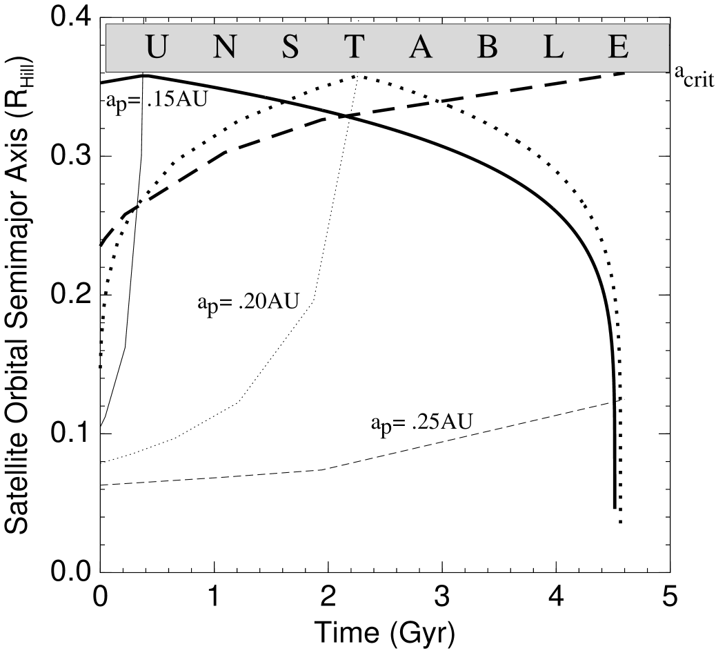
Figure 1: Satellite orbital semimajor axis versus time for the maximum-mass moon in three different hypothetical $4.6~{}\mathrm{Gyr}$ old $1~{}\mathrm{M_{\odot}}$, $1~{}\mathrm{M_{Jup}}$ planetary systems. The solid lines represent a system with a planet-star distance of $0.15~{}\mathrm{AU}$, with the thick and thin lines corresponding to the satellite semimajor axis and planet synchronous radius respectively. Tides between this planet and its star spin down the planet in short order, and the moon spends the majority of its lifetime evolving inward through tidal interactions with the planet. It is destroyed upon reaching the cloud tops of the planet. The dotted lines correspond to a system in which the planet-star separation is $0.20~{}\mathrm{AU}$; this planet is despun in just under half the age of the system. Thus its maximum-mass moon initially moves outward due to tidal influences, but later reverses direction due to the spindown of the planet and eventually crashes into it. This moon reverses direction at the critical semimajor axis (the outermost stable orbit point) because doing so maximizes its orbital lifetime. The dashed lines are for a planet orbital semimajor axis of $0.25~{}\mathrm{AU}$. The star’s tidal torques on the planet have less influence at this distance, and the planet does not despin sufficiently over its lifetime to reverse the orbital migration of its maximum-mass satellite. This satellite is lost into interplanetary space due to orbital instabilities.

3.1 Analytical Treatment

For a given semimajor axis of a moon, $a_{m}$, the migration rate is the same whether the moon is moving inward or outward (with the assumption that $Q_{p}$ is independent of the tidal forcing frequency $\Omega_{p}-n_{m}$), and the migration rate is much faster for satellites close to their parent planets. For both the inward- and outward-migrating categories, the total lifetime of a satellite ($T$) is well-characterized by the time necessary for a satellite orbit to traverse the entire region between the critical semimajor axis ($a_{m}=a_{crit}$) and the planet’s surface ($a_{m}=R_{p}$), (Murray & Dermott, 2000):

$$T=\frac{2}{13}\bigg{(}a_{crit}^{13/2}-R_{p}^{13/2}\bigg{)}\frac{Q_{p}}{3k_{2{p}}M_{m}R_{p}^{5}}\sqrt{\frac{M_{p}}{G}}~{}\mathrm{.}$$ (7)

Since $R_{p}\ll a_{crit}$ and the exponents are large, the $R_{p}$ term inside the parenthesis can be neglected. Substituting $a_{crit}=fR_{H}$ (Equation 6), allowing $T$ to be equal to the age of the system, and solving for $M_{m}$ collectively result in an analytical expression for the maximum possible extant satellite mass in both the inward and outward cases,

$$M_{m}\leq\frac{2}{13}\bigg{(}\frac{(fa_{p})^{3}}{3M_{*}}\bigg{)}^{13/6}\frac{M_{p}^{8/3}~{}Q_{p}}{3k_{2p}TR_{p}^{5}\sqrt{G}}~{}\mathrm{,}$$ (8)

which is the equation of the bottom, dot-dashed line in Figure 2. In the case of satellites that evolve outward then inward, the spindown of the planet is important. These moons can be saved temporarily by the reversal of their orbital migration. This reversal prolongs their lifetimes, but by less than a factor of two, because the satellite transverses the region where $a_{m}<a_{crit}$ twice. The upper mass limit for these satellites is

$$M_{m}\leq\frac{4}{13}\bigg{(}\frac{(fa_{p})^{3}}{3M_{*}}\bigg{)}^{13/6}\frac{M_{p}^{8/3}~{}Q_{p}}{3k_{2p}TR_{p}^{5}\sqrt{G}}~{}\mathrm{,}$$ (9)

and this limit is plotted as the upper dotted line in Figure 2.

We obtain the boundaries between the in, out-then-in, and out cases by comparing the time necessary to despin the planet to the age of the system. The time necessary to spin down the planet to the point that the synchronous radius becomes exterior to the critical semimajor axis is equal to (Guillot et al., 1996)

$$T_{spindown}=Q_{p}(\Omega_{p0}-\Omega_{p1})\left(\frac{R_{p}^{3}M_{p}}{GM_{*}^{2}}\right)~{}\mathrm{,}$$ (10)

where $\Omega_{p0}$ is the initial planetary rotation rate and $\Omega_{p1}$ is the rotation rate at which the planet’s synchronous radius is coincident with $a_{crit}$. At this point, from Kepler’s law we infer that

$$\Omega_{p1}=n_{crit}=\left(\frac{GM_{p}}{a_{crit}^{2}}\right)^{(1/3)}~{}\mathrm{.}$$ (11)

For the case where $T_{spindown}\ll T$ (where $T$ is the system liftime), the maximum-mass moon evolves inward and Equation 8 should be used. When the system age is greater than this spindown time ($T_{spindown}\gg T$), moons evolve outward and again Equation 8 is valid. However, when $T_{spindown}\sim T$, the reversal of satellite orbital migration is important and Equation 9 provides a more robust upper mass limit for surviving satellites.

These results for the maximum $M_{m}$ are limited by the requirement that the rate of angular momentum transfer between the planet and the satellite must be less than that between the planet and the star when $a_{m}$ is relatively large (i.e., $\tau_{p-*}>\tau_{p-m}$ in Equation 3) such that synchronization between the planet and moon does not occur. In the case of rocky satellites orbiting gaseous planets, this condition is met. For large moon-planet mass ratios or large $a_{p}$, this assumption breaks down, yielding a situation more closely resembling the isolated planet-satellite systems treated in Counselman (1973). In this case the planet and moon can become locked into a 1:1 spin-orbit resonance with each another, halting the satellite’s orbital migration and extending its lifetime. For extrasolar Jovian planets ($0.3\mathrm{M_{\odot}}<M_{p}<13.0\mathrm{M_{\odot}}$) this occurs when satellite masses become very large, i.e. greater than $8\mathrm{M_{\oplus}}$ for a $1\mathrm{M_{Jup}}$ planet. Such a moon is large enough to accrete hydrogen gas during its formation, however, and in such a case the system is better treated as a binary planet, taking into account the tidal torques of each body on the mutual orbit. We do not address that situation here.

We assume prograde, primordial satellites, but objects captured into orbit by a planet late in its life could also remain in orbit. We do not treat the physics of satellite capture, but the lifetimes of such moons would be affected by the same processes described above if prograde, and limited by inward migration like Neptune’s moon Triton (McCord, 1966) if retrograde. In the case of retrograde, captured moons, the following upper limit on their survival lifetime can be placed by rearranging Equation 8:

$$T_{max}=\frac{2}{13}\bigg{(}\frac{(f_{R}a_{p})^{3}}{3M_{*}}\bigg{)}^{13/6}\frac{M_{p}^{8/3}~{}Q_{p}}{3k_{2p}M_{m}R_{p}^{5}\sqrt{G}}~{}\mathrm{.}$$ (12)

Our analysis assumes a single satellite system. Inward-migrating moons could not be slowed significantly by entering into a resonance with another satellite further in because the interior satellite would be migrating faster (due to the $a_{m}^{-6}$ dependance of the torque in Equation 1), unless its mass is less than $.08~{}M_{m}$ (assuming a 2:1 resonance). Slowly-migrating moons exterior to the satellite in question cannot slow its orbital migration because objects in diverging orbits cannot be captured into resonances. However, outward-migrating satellites could have their lifetimes extended by entering into a resonance with an exterior neighbor through intersatellite angular momentum transfer (Goldreich, 1965), similar to the resonances currently slowing the outward migration of Io from Jupiter. Thus some outward-limited satellites above the mass limit derived in Equation 8 may still survive because of resonances entered into earlier in their lifetimes.

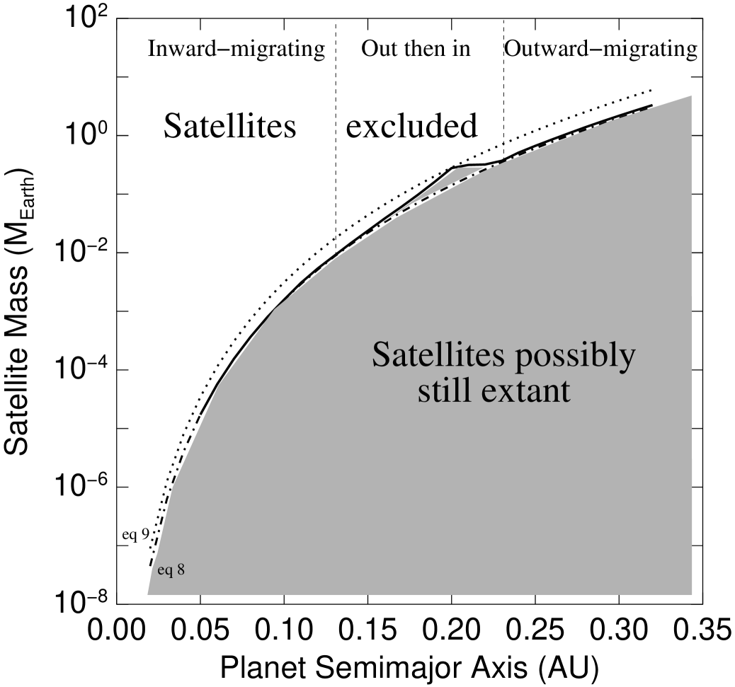
Figure 2: Stability diagram for satellites in a hypothetical $4.6~{}\mathrm{Gyr}$ old $1~{}\mathrm{M_{\odot}}$, $1~{}\mathrm{M_{Jup}}$ planetary system as a function of the planet’s orbital semimajor axis. The solid line represents the results from numerical integrations of Equations 3 and 4, and the broken lines are the analytical approximations given in Equations 8 (lower, dot-dashed) and 9 (upper, dotted). Satellites above this line are excluded, while those which lie below the line may or may not still exist depending on their specific orbital evolutionary histories. For this specific case, below $a_{p}\sim 0.15\mathrm{AU}$ satellite masses are limited by their inward migration, above $a_{p}\sim 0.23\mathrm{AU}$ by their outward migration, and in between by outward followed by inward migration with the reversal being the result of slowing planetary rotation.

3.2 Numerical Treatment

To verify the limits stipulated in Equations 8 and 9, we integrate Equations 3 and 4 numerically, from the initial rotation rate and semimajor axis until the satellite’s demise either through impact with the planet or through orbital escape. We use an adaptive stepsize Runge-Kutta integrator from Press et al. (1992) and have verified that it reproduces our analytical results for small satellite masses. We also assume that only $\Omega_{p}$ and $a_{m}$ change over time — other planetary parameters such as $Q_{p}$, $a_{p}$, $R_{p}$, and all others are taken to be constant for the length of the integration. The expected changes in the planet’s orbital semimajor axis $a_{p}$ over the course of the integration do not significantly affect the calculations, and larger planetary radii $R_{p}$ in the past would only serve to further reduce lifetime of a given satellite beyond what we have calculated here, pushing the upper surviving satellite mass lower.

For each planet, we determine the maximum satellite mass that could survive for the observed lifetime of the system by optimizing the initial semimajor axis of the satellite so as to maximize its lifetime and then tuning the satellite mass until this lifetime is equal to the system age. Sample evolutionary histories of this maximum mass satellite for a hypothetical $1M_{\odot}$, $1M_{Jup}$ system from each orbital evolutionary history category are shown in Figure 1. The numerically determined maximum mass as a function of planetary orbital semimajor axis is shown in Figure 2 as the solid line. These numerical results are consistent with our analytical upper mass limits from Equations 8 and 9.

4 IMPLICATIONS

4.1 Known Extrasolar Planets

In applying these results to the specific test case of the transiting planet HD209458b, we adopt the values $M_{*}=1.1~{}\mathrm{M_{\odot}}$, $M_{p}=0.69~{}\mathrm{M_{Jup}}$, $a_{p}=0.0468~{}\mathrm{AU}$, $T=5.0~{}\mathrm{Gyr}$ (Mazeh et al., 2000), and $R_{p}=1.35~{}\mathrm{R_{Jup}}$ (Brown et al., 2001) based on observational studies. We take $k_{2p}$ for the planet to be $0.51$, the value for an $n=1$ polytrope (Hubbard, 1984). The least constrained parameter is the tidal dissipation factor $Q_{p}$; for HD209458b we adopt $Q_{p}=10^{5}$, which is consistent with estimates for Jupiter’s $Q_{p}$ (Goldreich & Soter, 1966). However, $Q_{p}$ is not known precisely even for the planets in our own solar system, and the precise mechanism for the dissipation of tidal energy has not been established. $Q_{p}$ for extrasolar planets, and especially for ones whose interiors differ from Jupiter’s such as close-in giant planets (Burrows et al., 2000), may differ substantially from this value.

Because HD209458b was likely tidally spun down to synchronous rotation very quickly (Guillot et al., 1996), satellites around it are constrained by the infall time and we use Equation 8 to obtain an upper limit of $7\times 10^{-7}~{}\mathrm{M_{\oplus}}$ for their masses. Assuming a density of $\rho=3~{}\mathrm{g/cm^{3}}$, the largest possible satellite would be $70~{}\mathrm{km}$ in radius — slightly smaller than Jupiter’s irregularly-shaped moon Amalthea. These limits are consistent with the those placed on actual satellites observationally by Brown et al. (2001). It is possible for captured satellites to exist around HD209458b. Their lifetimes, however, would be exceedingly short — a $1\mathrm{M_{\oplus}}$ satellite could survive for only $30,000\mathrm{yr}$ (Equation 12), making the probability of detecting one low unless such captures are common.

We also calculate the maximum masses for surviving moons around other detected extrasolar planets; the results are in Table 2. We take the planet masses to be equal to the minimum mass determined by radial velocity monitoring, as the orbital inclination has not been reliably determined for any planet except HD209458b. We use the same $k_{2p}$ and $Q_{p}$ as we did for HD209458b, but take $R_{p}=R_{Jup}$ because the radii for these objects is unknown. For this table, we have only chosen planets whose orbital eccentricities are less than $0.10$ because Equation 6 applies only to planets in circular orbits. The critical semimajor axis for planets in noncircular orbits has not yet been determined, thus we leave the calculation of upper mass limits for satellites around these eccentric planets for future work.

4.2 Earth-like Moons

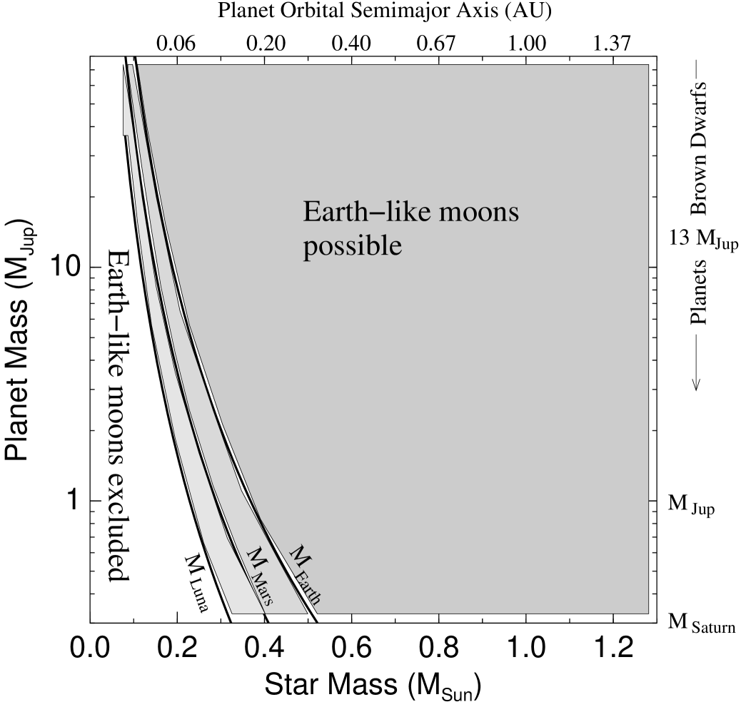
Figure 3: Stability of Earth-like moons. For stars of a given mass, we estimate a luminosity from Equation 13, and then calculate the limits on planet masses that allow for the stability of moons with insolation $F=1370~{}\mathrm{W~{}m^{-2}}$ and mass $1~{}\mathrm{M_{Luna}}$ (solid line, left), $1~{}\mathrm{M_{Mars}}$ (solid line, center), and $1~{}\mathrm{M_{Earth}}$ (solid line, right). Planets with the proper $a_{p}$ (top) and masses above the appropriate solid line might still harbor Earth-like satellites after $5~{}\mathrm{Gyr}$. For this plot, we have taken $R_{p}=R_{Jup}$, and as such the values are not valid for planets with masses less than $0.3~{}M_{Jup}$. Planet mass limits for very low mass stars where $M_{p}\sim M_{*}$ are also suspect. From this plot we infer that Earth-like satellites of Jovian planets are plausibly stable for $5~{}\mathrm{Gyr}$ around most stars with masses greater than $0.15~{}M_{\odot}$.

Our approach can also shed light on the issue of Earth-like satellites, which we define to be moons capable of supporting liquid water. Low-mass satellites do not fit this definition due to their inability to retain volatiles (Williams et al., 1997). Here we note that high-mass satellites may not survive for long periods around close-in planets because planets with low masses have smaller Hill spheres and therefore, for a given satellite mass, also have shorter maximum moon lifetimes. To calculate in general which giant planets might harbor Earth-like satellites, we use Equation 8 and constrain $a_{p}$ based on the insolation at the planet, $F$, relative to the Earth’s insolation $F_{\oplus}=1370~{}\mathrm{W~{}m^{-2}}$. We use the rough approximation (Hansen & Kawaler, 1994)

$$\frac{L_{*}}{L_{\odot}}=\left(\frac{M_{*}}{M_{\odot}}\right)^{3.5}$$ (13)

for the stellar luminosity, $L_{*}$, together with the insolation at the planet,

$$\frac{F}{F_{\oplus}}\frac{a_{p}^{2}}{a_{\oplus}^{2}}=\frac{L_{*}}{L_{\odot}}~{}\mathrm{,}$$ (14)

to fix the planet’s semimajor axis by solving for $a_{p}$. By plugging the resulting value for $a_{p}$ into Equation 8, we can exclude Earth-like moons around planets in systems that don’t satisfy the inequality

$$M_{p}\geq\left[\frac{39}{4}\left(\frac{f^{3}}{3}\right)^{-13/6}\frac{M_{m}k_{2p}TR_{p}^{5}\sqrt{G}}{Q_{p}}\right]^{3/8}\frac{M_{\odot}^{273/64}}{M_{*}^{221/64}}\left(a_{\oplus}^{2}\frac{F_{\oplus}}{F}\right)^{-39/32}~{}\mathrm{.}$$ (15)

Equation 15 is plotted in Figure 3 for the same values of $k_{2p}$, $Q_{p}$, and $f$ as we use for HD209458b, with $R_{p}=R_{Jup}$ and $T=5~{}\mathrm{Gyr}$.

Williams et al. (1997) found the lower limit $M_{m}\geq 0.12~{}\mathrm{M_{\oplus}}$ for moons that can retain volatiles over Gyr timescales. Using this mass, we find that Earth-like moons orbiting Jovian planets could survive for solar system lifetimes around stars with masses greater than $0.15~{}M_{\odot}$, and that Earth-mass satellites which receive similar insolation to the Earth are stable around all Jovian planets orbiting stars with $M_{*}>0.5~{}M_{\odot}$. Planets with masses less than $0.3~{}M_{Jup}$ differ in radius, $Q_{p}$, and interior structure from those with masses greater than $0.3~{}M_{Jup}$. In addition, for lower planet masses the planet/satellite mass ratio increases beyond the assumption of non-synchronization between the planet and moon. For these reasons, we do not treat the question of Earth-like satellites of ice-giant planets ($M_{p}<0.3\mathrm{M_{Jup}}$) here.

The radial-velocity planet most likely to harbor Earth-like moons is HD28185b because of its circular, $a_{p}=1\mathrm{AU}$ orbit around a star similar to the Sun withspectral type G5V and $L_{*}=1.09\mathrm{L_{\odot}}$ (Santos et al., 2001). Because the calculated upper satellite mass for this planet is above $8~{}\mathrm{M_{\oplus}}$, we can not rule out any satellite masses for this object. Thus, Earth-like moons with any mass could plausibly be stable around HD28185b.

4.3 Future Discoveries

Several missions to search for extrasolar planet transits by high-precision space-based photometry are in the planning stages and will, if launched, have the capability of detecting satellites (Sartoretti & Schneider, 1999). The probability that a given planet will transit across its parent star decreases with planetary orbital semimajor axis as $1/a_{p}$. Hence these surveys will preferentially detect planets in orbits close to their parent stars. However, we have shown that it is unlikely that these close-in objects will harbor satellites. Therefore satellite transits are most likely to be detected around planets orbiting at moderate distances from their parent star ( $0.3\mathrm{AU}\leq a_{p}\leq 2\mathrm{AU}$), even though planet transits are most likely at small orbital distances. If a satellite were detected, Equation 9 could be used to place limits on the planetary tidal dissipation parameter $Q_{p}$. By using extreme values of the lifetimes, masses, and possible values $Q_{p}$ that may exist, we estimate this process will not significantly affect planets more than $0.6\mathrm{AU}$ from their parent star, leaving any satellite systems they might posess intact.

Table 1: Satellite Semimajor Axes

Planet	Satellite	${a_{m}}/{R_{H}}$
Earth	Moon	0.257
Mars	Deimos	0.0216
Jupiter	Callisto	0.0354
Jupiter	Elara	0.221
Jupiter	Sinope	0.446
Saturn	Titan	0.0187
Saturn	Iapetus	0.0545
Saturn	Phoebe	0.198
Saturn	S/2000 S 9	0.283
Uranus	Oberon	0.00837
Uranus	Setebos	0.352
Neptune	Triton	0.003
Neptune	Nereid	0.0475

Note. — Orbital semimajor axes of selected solar system satellites are listed as a function of their their parent planet’s hill sphere radius, $R_{H}$.

Table 2: Constraints on Satellites around Selected Extrasolar Planets

Name	Star	M sin i	a	e	Max	Max	Reference
	Age	($M_{Jup}$)	(AU)		Moon	Moon
	(Gyr)				Mass	Radius
					($M_{\oplus}$)	(km)
HD83443b	(5)	0.35	0.038	0.08	$8\times 10^{-8}$	30	Mayor et al. (2000)
HD46375b	(5)	0.25	0.041	0.04	$6\times 10^{-8}$	30	Marcy et al. (2000a)
HD187123b	(5)	0.52	0.042	0.03	$6\times 10^{-7}$	60	Butler et al. (1998)
HD209458b	5	0.69	0.045	0	$7\times 10^{-7}$	70	Fischer et al. (2002)
HD179949b	(5)	0.84	0.045	0	$3\times 10^{-6}$	110	Tinney et al. (2001b)
HD75289b	(5)	0.42	0.046	0.053	$6\times 10^{-7}$	60	Udry et al. (2000)
BD -10 3166 b	(5)	0.48	0.046	0.05	$7\times 10^{-7}$	70	Butler et al. (2000)
T Boo b	2	4.1	0.047	0.051	$5\times 10^{-4}$	600	Butler et al. (1997)
51Pegasus b	(5)	0.44	0.051	0.013	$2\times 10^{-6}$	90	Marcy et al. (1997)
U And b	2.6	0.71	0.059	0.034	$2\times 10^{-5}$	190	Butler et al. (1999)
HD168746b	(5)	0.24	0.066	0	$2\times 10^{-6}$	100
HD130322b	(5)	1	0.088	0.044	$0.0008$	730	Udry et al. (2000)
55Cnc b	5	0.84	0.11	0.051	$0.001$	810	Butler et al. (1997)
Gl86b	(5)	3.6	0.11	0.042	$0.1$	3950	Queloz et al. (2000)
HD195019b	3.2	3.5	0.14	0.03	$0.8$	7090	Fischer et al. (1999)
GJ876c	5	1.9	0.21	0.1	$6$	14050	Marcy et al. (2001)
rho CrB b	10	1.1	0.23	0.028	$0.3$	5310	Noyes et al. (1997)
U And c	2.6	2.1	0.83	0.018	$\cdots$	$\cdots$	Butler et al. (1999)
HD28185b	(5)	5.6	1	0.06	$\cdots$	$\cdots$	Santos et al. (2001)
HD27442b	(5)	1.4	1.2	0.02	$\cdots$	$\cdots$	Butler et al. (2001)
HD114783b	(5)	1	1.2	0.1	$\cdots$	$\cdots$	Vogt et al. (2002)
HD23079b	(5)	2.5	1.5	0.02	$\cdots$	$\cdots$	Tinney et al. (2001a)
HD4208b	(5)	0.8	1.7	0.01	$\cdots$	$\cdots$	Vogt et al. (2002)
47UMa b	6.9	2.5	2.1	0.061	$\cdots$	$\cdots$	Fischer et al. (2002)
47UMa c	6.9	0.76	3.7	0.1	$\cdots$	$\cdots$	Fischer et al. (2002)

Note. — Upper satellite mass limits are determined with $Q_{p}=10^{5}$, $R_{p}=R_{Jup}$, and with $M_{p}=m\sin i$. Where no system lifetime was available in the literature, we have taken the system age to be $5~{}\mathrm{Gyr}$, and those cases are indicated by parenthesis. To obtain maximum moon radii, we assume $\rho=3~{}\mathrm{g~{}cm^{-3}}$. We can not place useful limits for those planets where maximum masses and radii are not listed. Planets with orbital eccentricities greater than $0.1$ are excluded due to the difficulty in determining the proper value of $f$. The planet data used to generate this table have been formed into a world wide web accessible database of extrasolar planets .

References

- Brown et al. (2001) Brown, T. M., Charbonneau, D., Gilliland, R. L., Noyes, R. W., & Burrows, A. 2001, ApJ, 552, 699
- Burns (1973) Burns, J. A. 1973, Nature Physical Science, 242, 23
- Burns (1986) Burns, J. A. 1986, in Satellites, ed. J. A. Burns, M. S. Matthews. (Tucson: University of Arizona Press), 117
- Burrows et al. (2000) Burrows, A., Guillot, T., Hubbard, W. B., Marley, M. S., Saumon, D., Lunine, J. I., & Sudarsky, D. 2000, ApJ, 534, L97
- Butler et al. (1999) Butler, R. P., Marcy, G. W., Fischer, D. A., Brown, T. M., Contos, A. R., Korzennik, S. G., Nisenson, P., & Noyes, R. W. 1999, ApJ, 526, 916
- Butler et al. (1998) Butler, R. P., Marcy, G. W., Vogt, S. S., & Apps, K. 1998, PASP, 110, 1389
- Butler et al. (1997) Butler, R. P., Marcy, G. W., Williams, E., Hauser, H., & Shirts, P. 1997, ApJ, 474, L115
- Butler et al. (2001) Butler, R. P., Tinney, C. G., Marcy, G. W., Jones, H. R. A., Penny, A. J., & Apps, K. 2001, ApJ, 555, 410
- Butler et al. (2000) Butler, R. P., Vogt, S. S., Marcy, G. W., Fischer, D. A., Henry, G. W., & Apps, K. 2000, ApJ, 545, 504
- Counselman (1973) Counselman, C. C. 1973, ApJ, 180, 307
- Fischer et al. (2002) Fischer, D. A., Marcy, G. W., Butler, R. P., Laughlin, G., & Vogt, S. S. 2002, ApJ, 564, 1028
- Fischer et al. (1999) Fischer, D. A., Marcy, G. W., Butler, R. P., Vogt, S. S., & Apps, K. 1999, PASP, 111, 50
- Goldreich (1965) Goldreich, P. 1965, MNRAS, 130, 159
- Goldreich & Soter (1966) Goldreich, P. & Soter, S. 1966, Icarus, 5, 375
- Guillot et al. (1996) Guillot, T., Burrows, A., Hubbard, W. B., Lunine, J. I., & Saumon, D. 1996, ApJ, 459, L35
- Hansen & Kawaler (1994) Hansen, C. J. & Kawaler, S. D. 1994, Stellar Interiors. Physical Principles, Structure, and Evolution. (New York: Springer-Verlag)
- Holman & Wiegert (1999) Holman, M. J. & Wiegert, P. A. 1999, AJ, 117, 621
- Hubbard (1984) Hubbard, W. B. 1984, Planetary Interiors (New York: Van Nostrand Reinhold Co.)
- Marcy et al. (2001) Marcy, G. W., Butler, R. P., Fischer, D., Vogt, S. S., Lissauer, J. J., & Rivera, E. J. 2001, ApJ, 556, 296
- Marcy et al. (2000a) Marcy, G. W., Butler, R. P., & Vogt, S. S. 2000a, ApJ, 536, L43
- Marcy et al. (1997) Marcy, G. W., Butler, R. P., Williams, E., Bildsten, L., Graham, J. R., Ghez, A. M., & Jernigan, J. G. 1997, ApJ, 481, 926
- Marcy et al. (2000b) Marcy, G. W., Cochran, W. D., & Mayor, M. 2000b, in Protostars and Planets IV. (Tucson: University of Arizona Press), 1285
- Mayor et al. (2000) Mayor, M., Naef, D., Pepe, F., Queloz, D., Santos, N. C., Udry, S., & Burnet, M. 2000, in ASP Conference Series, Vol. 202, in press
- Mazeh et al. (2000) Mazeh, T., Naef, D., Torres, G., Latham, D. W., Mayor, M., Beuzit, J., Brown, T. M., Buchhave, L., Burnet, M., Carney, B. W., Charbonneau, D., Drukier, G. A., Laird, J. B., Pepe, F., Perrier, C., Queloz, D., Santos, N. C., Sivan, J., Udry, S., & Zucker, S. 2000, ApJ, 532, L55
- McCord (1966) McCord, T. B. 1966, AJ, 71, 585
- Murray & Dermott (2000) Murray, C. D. & Dermott, S. F. 2000, Solar System Dynamics (New York: Cambridge University Press)
- Noyes et al. (1997) Noyes, R. W., Jha, S., Korzennik, S. G., Krockenberger, M., Nisenson, P., Brown, T. M., Kennelly, E. J., & Horner, S. D. 1997, ApJ, 483, L111
- Peale (1988) Peale, S. J. 1988, Icarus, 74, 153
- Press et al. (1992) Press, W. H., Teukolsky, S. A., Vetterling, W. T., & Flannery, B. P. 1992, Numerical recipes in C. The art of scientific computing (Cambridge: University Press)
- Queloz et al. (2000) Queloz, D., Mayor, M., Weber, L., Blécha, A., Burnet, M., Confino, B., Naef, D., Pepe, F., Santos, N., & Udry, S. 2000, A&A, 354, 99
- Santos et al. (2001) Santos, N. C., Mayor, M., Naef, D., Pepe, F., Queloz, D., Udry, S., & Burnet, M. 2001, A&A, 379, 999
- Sartoretti & Schneider (1999) Sartoretti, P. & Schneider, J. 1999, A&AS, 134, 553
- Tinney et al. (2001a) Tinney, C. G., Butler, R. P., Marcy, G. W., Jones, H. R. A., Penny, A. J., McCarthy, C., & Carter, B. D. 2001a, in astro-ph/0111255
- Tinney et al. (2001b) Tinney, C. G., Butler, R. P., Marcy, G. W., Jones, H. R. A., Penny, A. J., Vogt, S. S., Apps, K., & Henry, G. W. 2001b, ApJ, 551, 507
- Udry et al. (2000) Udry, S., Mayor, M., Naef, D., Pepe, F., Queloz, D., Santos, N. C., Burnet, M., Confino, B., & Melo, C. 2000, A&A, 356, 590
- Vogt et al. (2002) Vogt, S. S., Butler, R. P., Marcy, G. W., Fischer, D. A., Pourbaix, D., Apps, K., & Laughlin, G. 2002, ApJ, 568, 352
- Ward & Reid (1973) Ward, W. R. & Reid, M. J. 1973, MNRAS, 164, 21
- Williams et al. (1997) Williams, D. M., Kasting, J. F., & Wade, R. A. 1997, Nature, 385, 234