Kinematics of elliptical galaxies with a diffuse dust component – III. A Monte Carlo approach to include the effects of scattering

Abstract

This paper is the third one in a series, intended to investigate how the observed kinematics of elliptical galaxies are affected by dust attenuation. In Paper I and Paper II, we investigated the effects of dust absorption; here we extend our modelling in order to include the effects of scattering. We describe how kinematical information can be combined with the radiative transfer equation, and present a Monte Carlo code that can handle kinematical information in an elegant way.

Compared to the case where only absorption is taken into account, we find that dust attenuation considerably affects the observed kinematics when scattering is included. For the central lines of sight, dust can either decrease or increase the central observed velocity dispersion. The most important effect of dust attenuation, however, is found at large projected radii. The kinematics at these lines of sight are strongly affected by photons scattered into these lines of sight, which were emitted by high-velocity stars in the central regions of the galaxy. These photons bias the LOSVDs towards high line-of-sight velocities, and significantly increase the observed velocity dispersion and LOSVD shape parameters. These effects are similar to the expected kinematical signature of a dark matter halo, such that dust attenuation may form an alternative explanation for the usual stellar kinematical evidence for dark matter halos around elliptical galaxies.

We apply our results to discuss several other topics in galactic dynamics, where we feel dust attenuation should be taken into account. In particular, we argue that the kinematics observed at various wavelengths can help to constrain the spatial distribution of dust in elliptical galaxies.

1 Introduction

It is now generally accepted that elliptical galaxies are complicated objects, containing a variety of stellar populations, with a still poorly constrained dark matter content and a multi-component interstellar medium. The latter, and in particular the interstellar dust component, is not well understood. Nevertheless, knowledge about the dust component in galaxies is of fundamental importance. On the one hand, interstellar dust plays an active role in e.g. interstellar chemistry and star formation, and is therefore a key ingredient to understand galaxy structure and evolution. On the other hand, dust is very effective in absorbing and scattering UV and optical light, and knowledge about its presence, quantity and properties is necessary to correctly interpret any observable.

The far-infrared fluxes detected in the eighties by the IRAS satellite at 60 $\mu$m and 100 $\mu$m unveiled the presence of a substantial amount of dust in elliptical galaxies (Jura 1986; Bally & Thronson 1989; Knapp, Gunn & Wynn-Williams 1989). At that time, dust was already observed in the form of dust lanes and patches for a number of early-type galaxies (Hawarden et al. 1981; Ebneter & Balick 1985; Véron-Cetty & Véron 1988). Recent surveys indicate that dust extinction features are present in a large fraction of early-type galaxies (van Dokkum & Franx 1995; Ferrari et al. 1999; Tomita et al. 2000; Tran et al. 2001). These dust features, however, can not account for the high IRAS fluxes: the dust masses estimated from the IRAS measurements exceed those estimated from integrating the extinction features by nearly an order of magnitude (Goudfrooij & de Jong 1995). Moreover, the IRAS dust mass estimates are a lower limit for the true dust masses, because IRAS is not sensitive to cold dust, which emits the bulk of its radiation longwards of 100 $\mu$m. Calculations with a more realistic dust temperature distribution (Merluzzi 1998) and submillimeter observations (Fich & Hodge 1993; Wiklind & Henkel 1995) may indicate dust masses up to a magnitude higher than the IRAS estimates. The only plausible way to solve this dust mass discrepancy is to assume that the interstellar dust in elliptical galaxies exists as a two-component medium: the less massive component is optically visible in the form of dust lanes, whereas the more massive one is distributed diffusely over the galaxy (Goudfrooij & de Jong 1995).

Such a diffusely distributed dust distribution can be traced in two ways. The most obvious way is to map the thermal emission of the dust with spatially resolved far-infrared or submillimeter observations. A first effort to do this was undertaken by Leeuw, Sansom & Robson (2000), who used SCUBA imaging at 850 $\mu$m to look for thermal emission from dust in NGC 4374. Unfortunately, they could not detect a diffuse dust component, and found that the bulk of the 850 $\mu$m core emission is more likely the result of synchrotron radiation. Deeper imaging covering a larger wavelength range is necessary to constrain the spatial distribution of dust this way. Hopefully, the new generation of far-infrared and submillimeter instrumentation such as SIRTF and ALMA will help to clarify this issue.

A second way in which the diffuse dust component in elliptical galaxies can be traced is by colour gradients: because the extinction efficiency of dust grains decreases with wavelength, a diffuse dust component is expected to generate bluer colours at larger projected radii. Goudfrooij & de Jong (1995) and Wise & Silva (1996) found that the dust distributions, necessary to create the colour gradients observed in a sample of elliptical galaxies, are in reasonable agreement with their observed integrated FIR fluxes. However, various arguments seriously complicate the interpretation of colour gradients. Foremost, dust attenuation is not the only process that generates colour gradients: also age and metallicity variations can cause broadband colour gradients. Recently, Michard (2000) argued that the mean observed colour gradient ratios of a sample of elliptical galaxies are more likely the result of metallicity than of diffuse dust. And even if the dust attenuation were the only process responsible for the generation of colour gradients, tracing and quantifying the amount of dust would still be complicated. First, the dust is not located between the source and the observer, but well mixed with the stars. As a result, the amount of dust is not simply proportional to the amount of reddening (Disney, Davies & Phillipps 1989). Second, bluing due to scattering partly compensates the effects of reddening due to absorption, which suppresses the formation of large broad band colour gradients even if a substantial amount of dust is present (Witt, Thronson & Capuano 1992).

We have set up a program to investigate the effects of diffuse dust on the observed kinematics of elliptical galaxies. In the first two papers of this series (Baes & Dejonghe 2000, hereafter Paper I; Baes, Dejonghe & De Rijcke 2000, hereafter Paper II) we investigated how the light profile and the observed kinematics of elliptical galaxies are affected by dust absorption. In this series we extend our models by including the effect of scattering. In Section 2 we explain how the processes of dust absorption and scattering can affect the observables of galaxies. In particular, we explain how kinematical information can be included in the radiative transfer equation. In Section 3, we argue that a Monte Carlo method is the most straightforward way to do this. We describe the code we developed, with a special emphasis on the calculation of the observed kinematics. We use this code to investigate the effects of dust attenuation on the observed kinematics in elliptical galaxies. In Section 4 we present a set of simple elliptical galaxy models, consisting of a stellar and a dust component. We demonstrate how dust attenuation affects the light profile and observed kinematics of these models in Section 5. Section 6 is devoted to a discussion of our results, and finally, Section 7 sums up.

2 Radiative transfer in dusty galaxies

2.1 The general radiative transfer equation

The basis for any study of attenuation is the radiative transfer equation (RTE), which statistically describes the interaction between matter and light. In a general form, the time-independent RTE can be written as (Chandrasekhar 1960; Mihalas 1978)

$$\frac{{\text{d}}I}{{\text{d}}s}({\boldsymbol{r}},{\boldsymbol{k}})=j({\boldsymbol{r}},{\boldsymbol{k}})-\kappa({\boldsymbol{r}})\,I({\boldsymbol{r}},{\boldsymbol{k}}),$$ (1)

where $s$ is the path length, and $I({\boldsymbol{r}},{\boldsymbol{k}})$ represents the intensity at a position ${\boldsymbol{r}}$ into a direction ${\boldsymbol{k}}$. The right-hand side of the equation contains two terms that represent how the radiation field changes as a result of interactions with the matter. The first term, the total emissivity $j({\boldsymbol{r}},{\boldsymbol{k}})$ accounts for the sources of the radiation field. The second term, where $\kappa({\boldsymbol{r}})$ is the total opacity coefficient, represents the sinks. The specific form of both terms depends on which physical processes are taken into account, (e.g. stellar emission, absorption, scattering) and they can be complicated functions that depend on the intensity itself.

In a galaxy without dust attenuation, there are no sink terms, and the only source in the radiation field is the (isotropic) emission of photons by stars, such that $j({\boldsymbol{r}},{\boldsymbol{k}})=\ell({\boldsymbol{r}})$ where $\ell({\boldsymbol{r}})$ represents the stellar emissivity. If we take absorption by dust grains into account, a sink term must be added, which accounts for the loss of photons from the radiation field. The total opacity then equals the absorption coefficient, i.e. $\kappa({\boldsymbol{r}})=\kappa_{\text{abs}}({\boldsymbol{r}})$. In either of these situations, the RTE is a ordinary differential equation, and it can be solved by an integration along the line of sight.

Dust grains do not only absorb photons, they also scatter them, i.e. a number of photons are, as a result of an interaction with a dust grain, removed from their path and sent into another direction. This physical process is not a rare phenomenon: for typical Milky Way dust grains, the probability for scattering even slightly exceeds the probability for absorption in the optical wavelength range (Table 1). It is therefore obvious that scattering should be included in radiative transfer calculations. This will add two extra terms to the RTE. The first one is a sink term that accounts for the loss of photons scattered out of the beam. The total opacity will hence be the sum of the absorption coefficient and the scattering coefficient, $\kappa({\boldsymbol{r}})=\kappa_{\text{abs}}({\boldsymbol{r}})+\kappa_{\text{sca}}({\boldsymbol{r}})$. The second extra term is a source term that characterizes the gain of photons scattered into the beam. More precisely, this term will contain the contribution of photons that had another direction ${\boldsymbol{k}}^{\prime}$, but are now scattered into the direction ${\boldsymbol{k}}$. Generally, the distribution of angles after a scattering process are described by a scattering phase function $\Phi({\boldsymbol{r}},{\boldsymbol{k}},{\boldsymbol{k}}^{\prime})$, which describes the probability that a photon which comes from the direction ${\boldsymbol{k}}^{\prime}$ and is scattered at ${\boldsymbol{r}}$, will have ${\boldsymbol{k}}$ as its new direction. By convention, it is normalized as

$$\iint\frac{{\text{d}}\Omega^{\prime}}{4\pi}\,\Phi({\boldsymbol{r}},{\boldsymbol{k}},{\boldsymbol{k}}^{\prime})=1\qquad\text{for all ${\boldsymbol{r}}$ and all ${\boldsymbol{k}}$.}$$ (2)

The fraction of the intensity scattered from a solid angle ${\text{d}}\Omega^{\prime}$ around an arbitrary direction ${\boldsymbol{k}}^{\prime}$ into the direction ${\boldsymbol{k}}$ will therefore equal $\kappa_{\text{sca}}({\boldsymbol{r}})\,I({\boldsymbol{r}},{\boldsymbol{k}}^{\prime})\,\Phi({\boldsymbol{r}},{\boldsymbol{k}},{\boldsymbol{k}}^{\prime})\,{\text{d}}\Omega^{\prime}/4\pi$, such that the extra source term that has to be added to the RTE reads

$$j_{\text{sca}}({\boldsymbol{r}},{\boldsymbol{k}})=\kappa_{\text{sca}}({\boldsymbol{r}})\iint\frac{{\text{d}}\Omega^{\prime}}{4\pi}\,I({\boldsymbol{r}},{\boldsymbol{k}}^{\prime})\,\Phi({\boldsymbol{r}},{\boldsymbol{k}},{\boldsymbol{k}}^{\prime}).$$ (3)

It is convenient to introduce the scattering albedo $\omega$ as the ratio of the scattering coefficient to the total opacity coefficient,

$$\omega({\boldsymbol{r}})=\frac{\kappa_{\text{sca}}({\boldsymbol{r}})}{\kappa({\boldsymbol{r}})}=1-\frac{\kappa_{\text{abs}}({\boldsymbol{r}})}{\kappa({\boldsymbol{r}})}.$$ (4)

We finally find for the RTE,

$$\frac{{\text{d}}I}{{\text{d}}s}({\boldsymbol{r}},{\boldsymbol{k}})=\ell({\boldsymbol{r}})-\kappa({\boldsymbol{r}})\,I({\boldsymbol{r}},{\boldsymbol{k}})\\ +\omega({\boldsymbol{r}})\,\kappa({\boldsymbol{r}})\,\iint\frac{{\text{d}}\Omega^{\prime}}{4\pi}\,I({\boldsymbol{r}},{\boldsymbol{k}}^{\prime})\,\Phi({\boldsymbol{r}},{\boldsymbol{k}},{\boldsymbol{k}}^{\prime}).$$ (5)

The inclusion of scattering turns the RTE into a integro-differential equation, far more complicated than the ordinary differential equation if only absorption is taken into account. In particular, the scattering term is responsible for the coupling of the RTE along different paths: due to the integration over the angle, we cannot solve the RTE for a single path, but we have to solve it for all paths at the same time.

2.2 The geometry

The complexity of the RTE does not only depend on which physical processes are taken into account (the right-hand side), but also on the geometry of the system. Indeed, the path length appearing in the left-hand side of the RTE is in general a function of position and direction, i.e. $s=s({\boldsymbol{r}},{\boldsymbol{k}})$. As a consequence, the (time-independent) RTE is a partial differential equation with five independent coordinates (see e.g. Mihalas 1978). This complexity, however, is reduced if the system has symmetries. For example, in an axially symmetric geometry, the azimuthal dependence vanishes, such that only four independent coordinates need to be considered.

Particularly interesting is the spherical geometry, because in that case only two coordinates remain: the radius $r$ and the cosine $\mu$ of the angle between the direction ${\boldsymbol{k}}$ and the local radial direction. The aim of this paper is to provide a global picture of the effects of dust attenuation on the observed kinematics of elliptical galaxies, rather than modelling a specific, possibly geometrically complex object. For this goal, the assumption of spherical symmetry is satisfactory.

There are no ways to solve the general RTE (5) analytically, but several techniques have been developed to solve it numerically. And because many astrophysical systems can in a first approximation be considered spherically symmetric, many efforts have yet been spent on the RTE in a spherical geometry. The pioneering work started nearly 70 years ago (Kosirev 1934; Chandrasekhar 1934), and, in particular since the 1970s, a vast number of different approaches has been developed (e.g. Hummer & Rybicki 1971; Schmid-Burgk 1975; Witt 1977; Flannery, Roberge & Rybicki 1980; Yorke 1980; Rowan-Robinson 1980; Rogers & Martin 1984; Peraiah & Varghese 1985; Gros, Crivellari & Simonneau 1997). Most of these techniques, however, are not suitable for our needs, because it seems hard (and at least not obvious) to extend them such that they can handle kinematical information. Only for Monte Carlo methods, the kinematical information could be included in an elegant way.

2.3 Including kinematical information

As long as scattering is not taken into account, the inclusion of velocity information in the RTE is rather straightforward. Indeed, instead of taking into account the entire stellar emissivity, we can just consider the light from those stars whose velocity component in the direction of the observer equals $v_{\parallel}$. The emissivity of these stars is given by $\ell({\boldsymbol{r}})\,\phi({\boldsymbol{r}},{\boldsymbol{k}},v_{\parallel})$, where $\phi({\boldsymbol{r}},{\boldsymbol{k}},v_{\parallel})$ is the spatial LOSVD, i.e. the probability for a star at position ${\boldsymbol{r}}$ to have a velocity component $v_{\parallel}$ in the direction ${\boldsymbol{k}}$ (Appendix A). Solving the RTE with this emissivity, we obtain the LOSVDs observed in the plane of the sky. Hence, if either dust attenuation is completely neglected or only absorption by dust grains is taken into account, the observed LOSVDs can be calculated from the spatial LOSVDs through a single integration along the line of sight. Similar relations hold between the moments of the distribution function, and the moments of the LOSVDs, e.g. the observed velocity dispersion profile can be determined from the intrinsic velocity dispersions by a simple integration along the line of sight. For more details, we refer to Paper I.

\psfrag{*}{\small star}\psfrag{k0}{\small${\boldsymbol{k}}_{0}$}\psfrag{d}{\small dust grain}\psfrag{kobs}{${\boldsymbol{k}}_{\text{obs}}$}\psfrag{vsys}{${\boldsymbol{v}}_{\text{sys}}$}\psfrag{vd}{${\boldsymbol{v}}_{d}$}\psfrag{vs}{${\boldsymbol{v}}_{*}$}\psfrag{observer}{observer}\includegraphics[clip,width=199.16928pt]{kininfo.eps}

Figure 1: The inclusion of kinematical information in the radiative transfer equation. This figure shows the trajectory of a photon through the galaxy (undulating line): after being emitted by the star, it is scattered once before it leaves the galaxy. See text for more details.

When scattering is included, however, the inclusion of kinematical information becomes much more complicated, because the velocities of both the stars and the dust grains that scatter their light need to be taken into account. Consider, for example, Fig. 1. A photon with rest wavelength $\lambda_{0}$ is emitted by a star moving with a velocity ${\boldsymbol{v}}_{*}$ into a direction ${\boldsymbol{k}}_{0}$ (in a reference frame centered on the galaxy center). Assume this photon is scattered by a dust grain moving with velocity ${\boldsymbol{v}}_{d}$, and then scattered towards the observer. The wavelength ”detected” by the dust grain is determined by the relative velocity between star and dust grain, i.e. the dust grain detects a wavelength

$$\lambda=\lambda_{0}\left[1-\frac{({\boldsymbol{v}}_{*}-{\boldsymbol{v}}_{d})\cdot{\boldsymbol{k}}_{0}}{c}\right].$$ (6)

The dust grains scatters the photon coherently into the direction ${\boldsymbol{k}}_{\text{obs}}$, such that the wavelength detected by the observer equals

$$\lambda=\lambda_{0}\left[1-\frac{({\boldsymbol{v}}_{*}-{\boldsymbol{v}}_{d})\cdot{\boldsymbol{k}}_{0}}{c}\right]\left[1-\frac{({\boldsymbol{v}}_{d}+{\boldsymbol{v}}_{\text{sys}})\cdot{\boldsymbol{k}}_{\text{obs}}}{c}\right],$$ (7)

where ${\boldsymbol{v}}_{\text{sys}}$ is the system velocity with respect to the observer. The line-of-sight velocity $v_{\parallel}$ detected by the observer can be found from the relation

$$\lambda=\lambda_{0}\,\left[1-\frac{v_{\parallel}+{\boldsymbol{v}}_{\text{sys}}\cdot{\boldsymbol{k}}_{\text{obs}}}{c}\right],$$ (8)

which defines $v_{\parallel}$ and already incorporates the system velocity. Because the velocities of dust grains and stars in galaxies are very small compared the speed of light, second order terms in $v/c$ can be safely neglected, such that with (7) and (8),

$$v_{\parallel}={\boldsymbol{v}}_{*}\cdot{\boldsymbol{k}}_{0}+{\boldsymbol{v}}_{d}\cdot\left({\boldsymbol{k}}_{\text{obs}}-{\boldsymbol{k}}_{0}\right).$$ (9)

When more scattering events are involved in the photon’s trajectory, the relative velocities of each pair of subsequent dust grains have to be taken into account. If we denote the total number of scattering events with $M$, the velocities of the dust grains with ${\boldsymbol{v}}_{d_{i}}$ and the propagation directions with ${\boldsymbol{k}}_{i}$ (for $i=1\ldots M$), we obtain

$$v_{\parallel}={\boldsymbol{v}}_{*}\cdot{\boldsymbol{k}}_{0}+\sum_{i=1}^{M}{\boldsymbol{v}}_{d_{i}}\cdot\left({\boldsymbol{k}}_{i}-{\boldsymbol{k}}_{i-1}\right).$$ (10)

In general, therefore, the inclusion of kinematical information into radiative transfer problems is very complex. For our problem of dust attenuation in elliptical galaxies, however, we can make one assumption that reduces the complexity considerably: the summation in formula (10), i.e. the common contribution of the dust velocities, is in general negligible with respect to the first term, the contribution of the stellar velocity. Several arguments support this assumption. [1] It is reasonable to assume that the dust grains have smaller velocities than the stars in elliptical galaxies. Indeed, if the dust grains were to have large velocities, they would collide and heat up. However, the lion’s share of the dust in elliptical galaxies is assumed to be cold (Fich & Hodge 1993; Goudfrooij & de Jong 1995; Wiklind & Henkel 1995; Merluzzi 1998). [2] Scattering off interstellar dust is generally anisotropic, with a larger probability for forward scattering (see Section 4.2.2). In Appendix B we show that the anisotropic nature of scattering contributes to reducing the importance of the dust grain velocity terms in equation (10). [3] There is no reason why the velocity of dust grains in an elliptical galaxy would have a preferential direction. The individual terms in the summation in formula (10) will therefore have a random sign, and the summation will in the mean be washed out by multiple scattering.

As a consequence, we can write equation (10) simply as $v_{\parallel}={\boldsymbol{v}}_{*}\cdot{\boldsymbol{k}}_{0}$. Each photon hence carries the velocity component of the star in the direction of the emission of the photon.

3 Description of the Monte Carlo routine

3.1 Basic characteristics

We constructed a Monte Carlo code to solve our radiative transfer problem. Usually, the main argument against Monte Carlo methods is that it is computationally rather expensive compared to other methods (see e.g. Baes & Dejonghe 2001a). It has other advantages, however, which make it very competitive, in particular in an era when CPU time is not the most stringent limitation anymore. Important qualities of the Monte Carlo method are the possibility for a proper error analysis and a very wide flexibility. Nice examples of this flexibility are the ability to handle arbitrary geometries (Wolf, Fischer & Pfau 1998; Wood & Reynolds 1999; Gordon et al. 2001), the polarization of the scattered radiation (Code & Whitney 1995; Bianchi, Ferrara & Giovanardi 1996), the clumpiness of the interstellar medium (Witt & Gordon 1996; Bianchi et al. 2000), and the self-consistent heating and re-emission of the absorbed radiation (Wolf, Henning & Stecklum 1999; Bianchi, Davies & Alton 2000; Misselt et al. 2001). We make use of another possibility of the Monte Carlo method: its ability to include kinematical information in an elegant way. This possibility has recently been explored by Matthews & Wood (2001), who studied the effect of dust attenuation on the observed rotation curve in the spiral galaxies. Our modelling opens up the possibility to construct all LOSVDs and hence to investigate the entire observed kinematical structure of galaxies.

The principles of the Monte Carlo technique are outlined in detail by various authors (Cashwell & Everett 1959; Mattila 1970; Witt 1977; Yusef-Zadeh, Morris & White 1984; Fischer, Henning & Yorke 1994; Bianchi et al. 1996). Basically, the routine consists of following the individual trajectory of a very large number of photons through the galaxy. A photon’s history is given by a number of quantities such as the position and propagation direction at birth, the distance the photon travels before it interacts with a dust grain, the kind of this interaction, etc. Each of these quantities is described statistically by a random variable, taken from a particular probability density. Our approach is based on Witt (1977) and Bianchi et al. (1996). It includes the use of a continuous three-dimensional cartesian reference system (no grid). Furthermore, we use the classical tricks to optimize the routine: we assign a weight to each photon in order to avoid the loss of photons due to absorption, and we apply the forced first scattering mechanism to improve the statistics of the scattered radiation (Cashwell & Everett 1959; Witt 1977). The novelty of our Monte Carlo code is that it can calculate both photometric and kinematic data: not only the light profile, but also the LOSVDs and the projected kinematic moments. It simultaneously calculates these data in three modes: without dust attenuation, with only absorption taken into account and with dust attenuation fully taken into account. It is a monochromatic code, i.e. it calculates the observables in one single wavelength. If desired, the wavelength dependence of the results can be investigated by running the code various times at different wavelengths. We implemented the central wavelengths of the optical $U$, $B$, $V$, $R$, $I$ and the near-infrared $J$, $H$ and $K$ broadbands.

3.2 Calculation of the light profile

The light profile of the galaxy is constructed by simulating an imaging process. If a photon leaves the galaxy, we record the position of the last scattering event and the final propagation direction of the photon. Because in spherical symmetry, a path can be determined by its projected radius, we only need to record the projected radius of the photon’s final path. The registration of the photons is done by constructing a histogram of the photons leaving the galaxy as a function of $R$, where the contribution of each photon is measured by its weight (see Witt 1977).

3.3 Calculation of the LOSVDs

The Monte Carlo method provides an elegant possibility to include kinematical information. Indeed, we argued that the velocity information that a photon carries is essentially the velocity component of the star in the direction of the emission. This extra information can easily be included in the Monte Carlo routine. The only extension is that we do not only have to generate an initial position and propagation direction for each photon, but also a stellar velocity. The initial position and the stellar velocity have to be extracted in accordance with the phase space distribution function $F({\boldsymbol{r}},{\boldsymbol{v}})$, which represents the probability of finding a star at the position ${\boldsymbol{r}}$ with velocity ${\boldsymbol{v}}$. A practical way to do so, is following the strategy of Wybo & Dejonghe (1996), who generated sets of phase space coordinates of stars to create $N$-body representations of globular clusters. First, a random position ${\boldsymbol{r}}_{0}$ is determined from the stellar emissivity, and then a random stellar velocity ${\boldsymbol{v}}_{*}$ is generated from the three-dimensional probability density $p({\boldsymbol{v}})={\mathcal{L}}\,F({\boldsymbol{r}}_{0},{\boldsymbol{v}})/\ell({\boldsymbol{r}}_{0})$, using the acceptance-rejection method (Abramowitz & Stegun 1965; Press et al. 1989). Next, we determine a random emission direction ${\boldsymbol{k}}_{0}$, and determine the velocity component of ${\boldsymbol{v}}_{*}$ in the direction ${\boldsymbol{k}}_{0}$, i.e. $v_{\parallel}={\boldsymbol{v}}_{*}\cdot{\boldsymbol{k}}_{0}$. Given these initial conditions, we follow the photon until the exit conditions are satisfied, and calculate the projected radius of the final line of sight. The photon will then be stacked, according to its weight, in the appropriate bin in a two-dimensional array with axes $R$ and $v_{\parallel}$. This process is repeated this for a large number of photons and two-dimensional histograms are formed.

This method can be optimized in two ways. Firstly, we see that the velocity vector ${\boldsymbol{v}}_{*}$ does not show up in the Monte Carlo procedure itself, but only in the classification process. Moreover, we actually don’t need the entire information contained in the velocity ${\boldsymbol{v}}_{*}$: we only need the component $v_{\parallel}$ of the velocity in the direction ${\boldsymbol{k}}_{0}$. Therefore it is sufficient to generate a random $v_{\parallel}$ from the spatial LOSVD $\phi({\boldsymbol{r}}_{0},{\boldsymbol{k}}_{0},v_{\parallel})$, which represents the probability density of line-of-sight velocities for a star at position ${\boldsymbol{r}}_{0}$ in the direction ${\boldsymbol{k}}_{0}$. Instead of generating a three-dimensional velocity vector for each photon in the beginning of the Monte Carlo cycle, it is hence sufficient to generate one single line-of-sight velocity component. This saves many random number generations and distribution function evaluations, which are costly processes.

A second optimization eliminates the generation a $v_{\parallel}$ altogether. Instead of generating one single random $v_{\parallel}$, we can, for each bin in the velocity direction, calculate the probability that the line-of-sight velocity will fall in that bin. If the boundaries of a bin are given by $v_{\parallel,j-1}$ and $v_{\parallel,j}$, this probability equals

$$\int_{v_{\parallel,j-1}}^{v_{{\parallel,j}}}\phi({\boldsymbol{r}}_{1},{\boldsymbol{k}}_{0},v_{\parallel})\,{\text{d}}v_{\parallel}\\ \approx\frac{1}{2}\,\frac{\phi({\boldsymbol{r}}_{1},{\boldsymbol{k}}_{0},v_{\parallel,j-1})+\phi({\boldsymbol{r}}_{1},{\boldsymbol{k}}_{0},v_{\parallel,j})}{v_{\parallel,j}-v_{\parallel,j-1}}.$$ (11)

For each photon, we assign a weighted value to each velocity bin corresponding to the final projected radius, which gives better statistics than dropping the photon in a single bin.

3.4 Calculation of the projected kinematics

Of course, we are not able anymore to write down a direct connection between the intrinsic moments of the distribution function and the projected moments on the plane of the sky, contrary to the absorption-only case (Paper I). Instead, we will calculate the projected moments directly from the obtained LOSVDs. The projected kinematics we consider are the mean projected velocity $\bar{v}_{p}$, the projected velocity dispersion $\sigma_{p}$, the skewness $k_{3}$, the kurtosis $k_{4}$, and the lowest order Gauss-Hermite coefficients $h_{3}$ and $h_{4}$. Note, however, that for spherically symmetric non-rotating galaxies all odd moments vanish, i.e. $\bar{v}_{p}=k_{3}=h_{3}=0$.

3.5 Error analysis

Obviously, a reliable error analysis is necessary to estimate the accuracy of the results. But it will be even more important in a later stage. Indeed, we are presently incorporating this radiative transfer mechanism into the QP program (Dejonghe 1989), a code for the dynamical modelling of gravitating systems. Therefore, it is necessary that we can dynamically evaluate the error bars on any observable: the program has to be able to calculate any observable with an preset accuracy, required by either the user or another part of the code itself. Monte Carlo methods satisfy this need: they can keep on adding photons until any accuracy requirement is satisfied.

The determination of the errors is easy for observables that are directly proportional to the number of photons detected in the bins, e.g. the intensity. Because of the Poisson character of the noise, the error bars on these quantities can be directly calculated from the square root of the number of photons. The observed kinematics we calculate, however, are not directly proportional to number of photons obtained in the bins, such that we cannot adopt this simple procedure. Therefore, we estimate the error on our observables using an alternative method. Assume we have calculated a value $f$ for a given observable (either photometrical or kinematical) after a run with $N$ photons. We divide the total number of photons in $M$ subsets, and for each of these subsets, we calculate the corresponding observable $f_{i}$. The uncertainty on $f$ is estimated as,

$$\Delta f=\left[\frac{1}{M}\sum_{i=1}^{M}(f_{i}-f)^{2}\right]^{1/2}.$$ (12)

Typically, we set $M=100$, and we adopt a minimum number of $10^{6}$ photons, i.e. $10^{4}$ photons per subset.

4 The galaxy models

To investigate the effects of dust attenuation on the light profile and the observed kinematics, we will adopt a set of dusty galaxy models, similar to those in Paper I and Paper II. They are spherically symmetric, and consist of a stellar and a dust component.

4.1 The stellar component

For the stellar component we use a self-consistent Plummer model (Plummer 1911; Dejonghe 1987), defined by the potential-density pair

$$\psi(r)=\frac{GM}{\sqrt{r^{2}+c^{2}}},$$ (13a)

$$\rho(r)=\frac{3M}{4\pi}\,\left(1+\frac{r^{2}}{c^{2}}\right)^{-5/2}.$$ (13b)

We adopt a core radius $c=5$ kpc, a total mass $M=6\times 10^{11}$ M_⊙ and a (constant) mass-to-light ratio $\Upsilon=4$ $\Upsilon_{\odot}$, such that the total emitted luminosity equals ${\mathcal{L}}=1.5\times 10^{11}$ L_⊙. As in Paper I, we consider different Plummer models, each with a different value for the parameter $q$, which describes the internal anisotropy of the stellar orbits. We adopt three different models: a radial model ($q=2$), the isotropic model ($q=0$) and a tangential model ($q=-6$). These are the same values as in Paper I, except that we replace the radial model with $q=1$ by the model with $q=2$. The reason for preferring $q=2$ above $q=1$ has a computationally nature: the spatial LOSVDs can be calculated analytically for $q=2$, whereas this is not possible for the $q=1$ model (Appendix A).

4.2 The dust component

As shown in Section 2.1, a complete characterization of the dust component requires a specification of the opacity $\kappa(r)$, the albedo $\omega(r)$ and the scattering phase function $\Phi(r,{\boldsymbol{k}},{\boldsymbol{k}}^{\prime})$. The opacity sets the total amount of dust and its spatial distribution, whereas the other two quantities describe the optical properties at a given distance to the galaxy centre. In order to limit the number of parameters in our model, we will assume that the optical properties of the dust grains are the same all over the galaxy, such that the albedo and the phase function become independent of $r$. We will return to this assumption in Section 5.3.3.

4.2.1 The dust distribution

We adopt the same family of dust components considered in Paper I and Paper II, characterized by the dust number density

$$n(r)=n_{0}\left(1+\frac{r^{2}}{c^{2}}\right)^{-\alpha/2},$$ (14)

where $n_{0}$ is the dust density at the center of the galaxy, and $c$ and $\alpha$ determine the actual shape of the dust distribution. Because the effect of varying $\alpha$ and $c$ are roughly similar, we restrict ourselves to varying the dust exponent $\alpha$, and we fix the dust core radius to $c=5$ kpc, equal to the stellar core radius. The variation of $\alpha$ still allows us to explore a large variety of star-dust geometries: small values of $\alpha$ correspond to centrally concentrated distributions, whereas for large $\alpha$ the distribution is shallower (Paper I).

At a fixed wavelength $\lambda$, the opacity function $\kappa_{\lambda}(r)$ can be derived from the dust density by multiplication with the (wavelength-dependent) dust cross-section $s_{\lambda}$. To characterize the dust distribution at a given wavelength, we thus need three parameters: the dust exponent $\alpha$, the central dust number density, and the dust cross-section $s_{\lambda}$. It is more convenient, however, to use another, equivalent, set of parameters. Indeed, if the opacity function is known at one particular wavelength, it can be determined at any other wavelength. Usually, the V-band is used as the reference wavelength. We can then write $\kappa_{\lambda}(r)=X_{\lambda}\,\kappa_{V}(r)$, where $X_{\lambda}\equiv s_{\lambda}/s_{V}$ is the extinction coefficient, relative to the V band. It is then customary to introduce the total V-band optical depth as

$$\tau_{V}=\int_{0}^{\infty}\kappa_{V}(r)\,{\text{d}}r.$$ (15)

If we use the triplet $(\tau_{V},\alpha,X_{\lambda})$ as parameters, the opacity at an arbitrary wavelength $\lambda$ can be written as

$$\kappa_{\lambda}(r)=\frac{2}{\sqrt{\pi}}\,\frac{\Gamma\left(\frac{\alpha}{2}\right)}{\Gamma\left(\frac{\alpha-1}{2}\right)}\,\frac{X_{\lambda}\tau_{V}}{c}\,\left(1+\frac{r^{2}}{c^{2}}\right)^{-\alpha/2}.$$ (16)

4.2.2 The phase function

We can safely assume that the phase function does not depend independently on the four variables $({\boldsymbol{k}},{\boldsymbol{k}}^{\prime})$, but only on the angle between the two directions ${\boldsymbol{k}}$ and ${\boldsymbol{k}}^{\prime}$. Setting ${\boldsymbol{k}}\cdot{\boldsymbol{k}}^{\prime}=\cos\alpha$, we can write the phase function as $\Phi(\cos\alpha)$. Probably the most widely adopted phase function that can describe anisotropic scattering is the one named after Henyey & Greenstein (1941). It has been derived empirically, as a description of the scattering of light in reflection nebulae in the Galaxy, and has a simple analytical form,

$$\Phi(\cos\alpha)=\frac{1-g^{2}}{(1+g^{2}-2g\cos\alpha)^{3/2}}.$$ (17)

This family of phase functions contains the so-called asymmetry parameter $g$, which is a measure for the anisotropy of the scattering. In particular, for $g=0$ the scattering is isotropic, whereas for $g=1$ the scattering is completely forward.

4.2.3 The optical properties

Table 1: The adopted optical properties of the dust grains, at the central wavelengths of the standard optical and near-infrared wavebands. Tabulated are the relative extinction coefficient $X_{\lambda}$, the scattering albedo $\omega_{\lambda}$ and the asymmetry parameter $g_{\lambda}$.

band	$\lambda$ (nm)	$X_{\lambda}$	$\omega_{\lambda}$	$g_{\lambda}$
$U$	360	1.52	0.63	0.65
$B$	440	1.32	0.61	0.63
$V$	550	1.00	0.59	0.61
$R$	700	0.76	0.57	0.57
$I$	850	0.48	0.55	0.53
$J$	1250	0.28	0.53	0.47
$H$	1650	0.167	0.51	0.45
$K$	2200	0.095	0.50	0.43

From the previous subsections, we see that, in total, we need five parameters to describe a dust component at a given wavelength $\lambda$: the V-band optical depth $\tau_{V}$, the dust exponent $\alpha$, the relative extinction coefficient $X_{\lambda}$, the scattering albedo $\omega_{\lambda}$ and the asymmetry parameter $g_{\lambda}$. In principle, all of these parameters could be considered as free parameters. In order to limit the degrees of freedom, however, we decided not to consider the optical properties of the dust as a set of free parameters, but to use a fixed set of dust parameters. The values we use are listed in Table 1. They are taken from Gordon, Calzetti & Witt (1997), who derived them from an interpolation between a large set of empirical data of typical Milky Way dust. Notice in particular that the scattering albedo does not vary greatly within the optical and near-infrared regime. It is always slightly greater than 0.5, i.e. the probability for absorption is always slightly smaller than the probability for scattering.

4.3 A template model

Our models contain three parameters, the orbital structure parameter $q$, the $V$-band optical depth $\tau_{V}$ and the dust exponent $\alpha$. By varying these, we can describe a set of dusty elliptical galaxy models with a large variety in internal dynamics, dust content and star-dust geometry. We apply the same strategy as in Paper I to present the results of our modelling. First, we keep the geometry of the dust component fixed, and we investigate how dust distributions with various optical depths affect the light profile and observed kinematics of our three Plummer models. Next, we keep the optical depth fixed and consider a set of star-dust geometries by varying the dust exponent $\alpha$.

We therefore require a template model, where we can vary one parameter while keeping the other one fixed. For the optical depth of this template model, we choose $\tau_{V}=1$, a value that could be in agreement with both the far-infrared emission and the colour gradients in elliptical galaxies (Witt et al. 1992; Goudfrooij & de Jong 1995; Wise & Silva 1996). For the dust geometry of the template model, we adopt a modified Hubble profile, characterized by setting $\alpha=3$. It is shallower than the stellar distribution, which seems indicated by colour gradient models (Wise & Silva 1996). As a note we would like to stress that both the optical depth and geometry of the diffuse dust component in elliptical galaxies are very poorly known, apart from the solid result that FIR emission indicates that it is present. We return to this issue in Section 6.2.

Finally, we need to choose a template wavelength to present our results. Because the present paper focuses on the effects of dust attenuation on the observed kinematics, and because most of the kinematical observations are presently conducted at optical wavelengths, we will work in the $V$ band, unless mentioned otherwise.

5 Results

5.1 Putting the method to the test

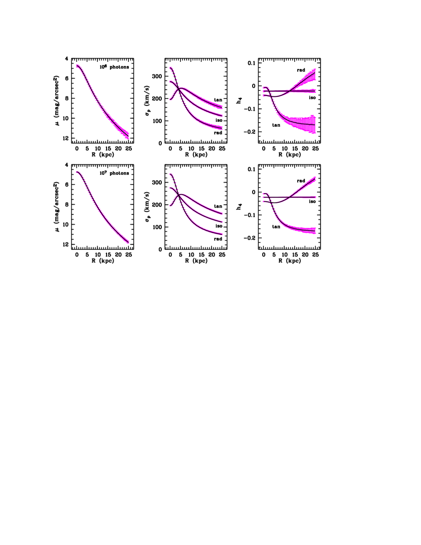
Figure 2: A comparison of the results of the Monte Carlo code in nodu mode (grey curves with error bars) and the corresponding analytical results (black lines). The upper and lower panels correspond to different values for the total number of emitted photons. Shown are the surface brightness profile, the projected velocity dispersion and the $h_{4}$ profile, for the three different orbital modes considered.

The Monte Carlo routine yields results in three modes, the nodu, abso and dust modes. Whereas we are of course mainly interested in the dust results, the other data sets are useful as a check for the accuracy of our results. If dust is not taken into account, the light profile and the projected kinematics can be calculated analytically for the galaxy models we consider (Dejonghe 1987). If only dust absorption is taken into account, they can be calculated through one single quadrature (Paper I). In Fig. 2 we compare the results of our Monte Carlo code with the corresponding analytical results, for two different values of $N$, the total number of emitted photons. Even for $N$ as low as $10^{6}$, the minimum number of photons we consider, the analytical results are very well reproduced, and are everywhere within the error bars.

5.2 The light profile

5.2.1 Dependence on the optical depth

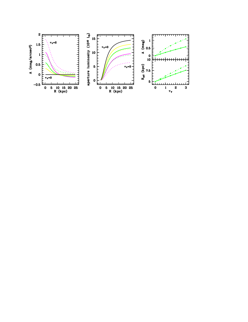
Figure 3: The effects of dust attenuation on the light profile, as a function of the optical depth. The left panel shows the attenuation profile of the galaxy, i.e. the fraction of the light output attenuated by the dust in magnitude units. It is shown for absorption only (dashed lines), and for full attenuation (solid lines), for optical depths $\tau_{V}=0,\tfrac{1}{2},1$ and $2$ – only the extreme ones are labelled. The middle plot shows the cumulative luminosity function, i.e. the fraction of the total emitted luminosity detected inside an aperture of radius $R$. The plots on the right-hand side show the effect of dust attenuation on the total attenuation and the effective radius, as a function of optical depth.

In Fig. 3 we demonstrate how the light profile is affected when both absorption and scattering are included. In the center of the galaxy (where the lines of sight contain most of the dust), the attenuation is strongest, and the attenuation decreases as one goes to the outer regions. As a consequence, also the apparent luminosity decreases, and the apparent size of the core (as measured by the effective radius $R_{e}$) increases as a function of $\tau_{V}$.

Within the first few kpc, dust attenuation has at first order the same effect on the light profile as absorption alone. Roughly, the effects of a attenuating dust component with optical depth $\tau_{V}$ can be approximated by a purely absorbing dust component with effective optical depth $\tau_{V}/2$. This approximation has a natural explanation: it follows from assuming that the scattering is purely forward. Indeed, the phase function corresponding to forward scattering is a simple Dirac delta function, $\Phi({\boldsymbol{k}},{\boldsymbol{k}}^{\prime})=4\pi\,\delta({\boldsymbol{k}}-{\boldsymbol{k}}^{\prime})$, and substituting this into the RTE (5), we find

$$\frac{{\text{d}}I}{{\text{d}}s}({\boldsymbol{r}},{\boldsymbol{k}})=\ell({\boldsymbol{r}})-(1-\omega)\,\kappa({\boldsymbol{r}})\,I({\boldsymbol{r}},{\boldsymbol{k}}).$$ (18)

This radiative transfer problem is completely analogous to a radiative transfer problem where only absorption is accounted for, but where the optical depth of the dust component is diminished with a factor $1-\omega\approx\tfrac{1}{2}$. This approximation is an appealing way to estimate the effects of scattering without elaborate and costly radiative transfer calculations. An argument in favour of this approximation is that multiple scattering events tend to wash out the effects of anisotropy of the scattering phase function. Hence, in media with a large opacity, any phase function can in principle be adopted, including the degenerate one corresponding to forward scattering (e.g. Di Bartolomeo, Barbaro & Perinotto 1995).

However, the effects of scattering should never be underestimated. In a previous study on the RTE in plane-parallel geometry, we investigated several ways often used in the literature to approximate scattering (Baes & Dejonghe 2001b). One of our main conclusions was that none of these methods provides a satisfactory approximation to the exact solution. The reason is that the physical process of scattering has a completely different nature than absorption, because it changes the path along which the photons propagate. The effect of scattering is that photons have a preferential direction in which to leave the galaxy. In a plane-parallel geometry, photons prefer the face-on direction to leave the galaxy, because when a photon is scattered into that direction, its chances to leave the galaxy are larger (the optical depth along the path is shorter) than when it is scattered into inclined directions. An analogous reasoning holds for spherical geometry, where photons will generally prefer large projected radii to leave the galaxy. As a consequence, the net effect of scattering is that photons are scattered out of lines of sight close to the center of the galaxy, into lines of sight with a large projected radius. In the outer regions of the galaxy, these extra photons will reduce the loss of radiation due to absorption. At very large projected radii, the attenuation will even be negative, i.e. the galaxy will even appear brighter than when dust extinction is not taken into account (Fig. 3). These results are in agreement with those found by Wise & Silva (1996), and they will be very important when we investigate the full effects of attenuation on the observed kinematics.

5.2.2 Dependence on the dust geometry

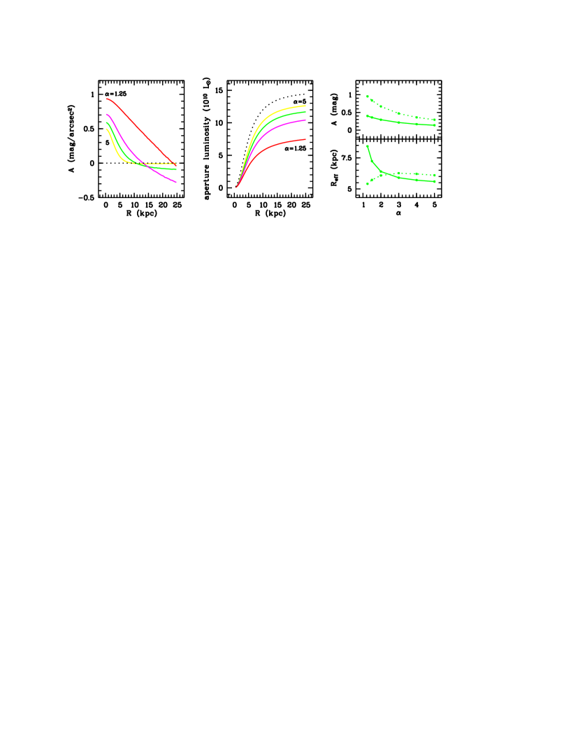
Figure 4: The effects of dust attenuation on the light profile, as a function of the dust geometry. The four panels in this figure are analogous to those in Fig. 3. The models shown here all have $\tau_{V}=1$, but different values for $\alpha$. The values shown are $\alpha=1.25$, 2$,3$ and 5. The black dotted lines in the left and middle panels correspond to the model without dust attenuation. The grey dotted lines on the right-hand side represent models with only absorption taken into account, as in Fig. 3.

In Fig. 4 we show the effects of varying the dust exponent on the light profile of our galaxy models. In the central regions of the galaxy, the combined effects of scattering and absorption on the light profile can roughly be approximated by pure absorption with an effective optical depth $\tau_{V}^{\text{eff}}=(1-\omega)\,\tau_{V}$. Therefore, the dependence on the dust exponent are similar to those when absorption only is taken in to account (Paper I): the attenuation is stronger for extended dust distributions ($\alpha$ small) than for centrally concentrated ones ($\alpha$ large). Because the central regions emit most of the light and therefore dominate the total observed luminosity, also the total attenuation will decrease as a function of $\alpha$.

At large projected radii, the dust has another effect on the light profile: the net effect is that photons scattered into these lines of sight cause a negative attenuation, i.e. the galaxy appears brighter. This effect should be stronger for extended dust distributions, because these distributions imply more dust in the outer regions of the galaxy, and hence an enhanced probability to be scattered into the outer lines of sight. This can indeed be observed in Fig. 4. In particular, this negative attenuation is nearly non-existent for a model where dust and stars have the same spatial distribution ($\alpha=5$), whereas it is clearly noticeable if the dust distribution is shallower than the stellar distribution.

5.3 The observed kinematics

5.3.1 Dependence on the optical depth

In an optically thin galaxy, the LOSVD is formed by summing the contribution of the line of sight velocities of all stars that are situated along that line of sight. If absorption is included in the projection process, still the same stars on the line of sight contribute to the LOSVD, but the contribution of each star is weighted by the amount of starlight that is able to survive the absorption and reach the observer. The net effect is that, for a given line of sight, the stars at the outer parts of the line of sight contribute relatively more to the LOSVD than the stars in the central parts (Paper I). Because the largest line-of-sight velocities along a given line of sight are usually found around the tangent point, the LOSVDs will be biased towards smaller velocities. In particular, the projected velocity dispersion generally decreases if absorption is taken into account. Only for the outer lines of sight of galaxies with a very radially anisotropic orbital structure, the largest line-of-sight velocities are found in the outer regions. Indeed, the stars at the tangent point have small line-of-sight velocities, because their (radial) orbits are nearly perpendicular to the line of sight. We showed in Paper I that the effects of dust absorption on the LOSVDs are only considerable for large optical depths ($\tau_{V}>5$), which are probably not appropriate for elliptical galaxies.

If scattering is taken into account, the situation changes drastically. The net effect of scattering, at least for the light profile, is that photons are taken away from the central lines of sight and sent into lines of sight at larger projected radii. Now consider a photon that is emitted by a star near the center of the galaxy, and that, after one or several scattering events, propagates towards the observer at a large projected radius. Although this photon will contribute to the LOSVD at this large projected radius, it carries the velocity information from the emitting star. Notice that this star does not physically belong to that line of sight. Hence, when scattering is taken into account, the LOSVDs aren’t LOSVDs anymore in the strict meaning of the word: the LOSVD at a certain line of sight can contain information of stars at totally different lines of sight. More generally, every single star in the galaxy will contribute to every single LOSVD, whereby its contribution will be weighed by the number of photons that leave the galaxy along that line of sight.

Beside the photons that disappear from the line of sight due to attenuation, we hence also have to account for the photons scattered into the line of sight, which contribute the additional kinematical information from stars that physically don’t belong there. How this process affects the LOSVDs is more complex than the effects due to the photons taken away from the line of sight. In particular, this effect is different for lines of sight that pass through the center of the galaxy ($R\approx 0$) and lines of sight at larger projected radii ($R\gg c$).

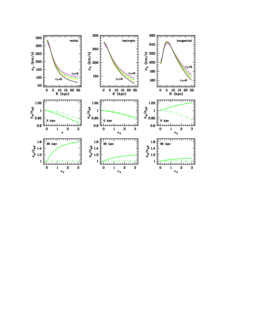
Figure 5: The effects of dust attenuation on the observed velocity dispersion, as a function of the optical depth. In the top panels, the projected velocity dispersion profiles are plotted, for different values of $\tau_{V}$. We have used the same values of $\tau_{V}$ and the same layout as in Fig. 3. The left, middle and right columns correspond to our radial, isotropic and tangential models respectively. The three panels on the middle row show the central projected velocity dispersion as a function of $\tau_{V}$. The values are normalized by $\sigma_{p,0}$, the central projected velocity dispersion in an optically thin galaxy. The solid lines represent the effect of dust attenuation, whereas in dashed lines we show the effects of absorption only. Analogously, the three bottom panels show the effects of dust attenuation, respectively absorption, on the normalized projected velocity dispersion at $R=25$ kpc.

If scattering is not taken into account, the LOSVD at the central line of sight $R=0$ only contains information on the radial velocity component of stars, because along the central line of sight $v_{\parallel}=v_{r}$. Because the vast majority of the stars along this line of sight reside in the central regions, the central LOSVDs will be dominated by the distribution of radial velocities in the galaxy center. If scattering is included, the central line of sight will also contain photons scattered into it, that would normally leave the galaxy at a larger projected radius. The vast majority of these photons will also originate from near the central region, but the line-of-sight velocities carried by them are not necessarily the radial velocity components of the stars that emitted them. These photons contaminate the LOSVD with tangential velocities: instead of containing pure radial velocity information, it will reflect a mix of radial and tangential components. As a consequence, the effect of scattering will depend on the ratio of radial to tangential velocity components in the central regions of the galaxy, i.e. on the orbital structure. In the panels on the middle row in Fig. 5, we plot the effect of increasing optical depth on the central projected velocity dispersion.

For isotropic galaxies, radial and tangential velocities are in balance throughout the galaxy, such that the photons scattered into the central lines of sight will hardly affect the LOSVD. The total effect of attenuation on the central LOSVDs will be dominated by the absorption effect, i.e. a bias towards smaller line-of-sight velocities. In particular, the central projected dispersion decreases if dust is taken into account, in a very similar way as when only absorption is taken into account.

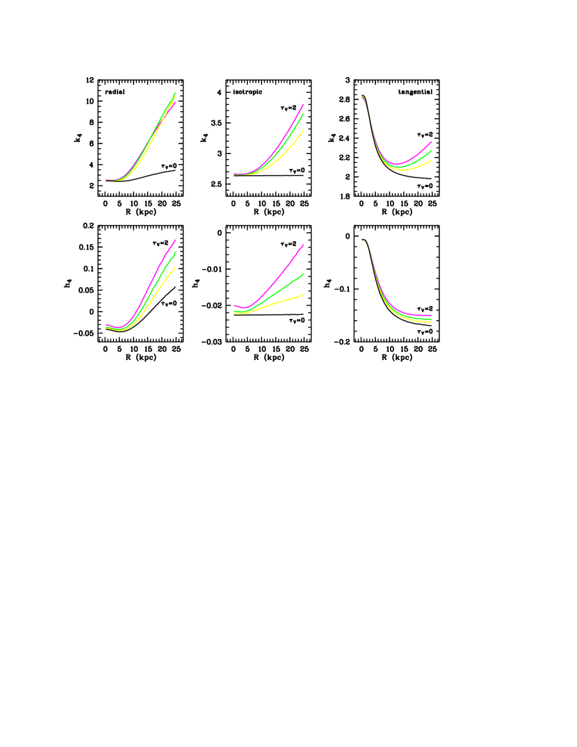
Figure 6: The effects of dust attenuation on the observed LOSVD shape, parametrized by the kurtosis $k_{4}$ and Gauss-Hermite $h_{4}$ coefficient, as a function of the optical depth. As in Fig. 5, the left, middle and right columns correspond to the radial, isotropic and tangential models respectively. The adopted optical depths and layout are similar to those used in Fig. 3.

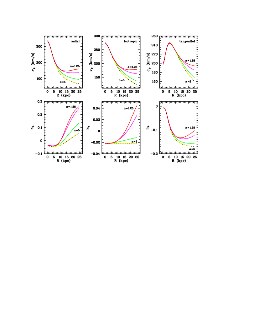
Figure 7: The effects of dust attenuation on the observed kinematics, as a function of the dust geometry. Shown are the projected dispersion profile and the $h_{4}$ profile, for different values of the dust exponent $\alpha$. The presented models and the layout are the same as in Fig. 4. As in the previous figures, the three column correspond to the three different Plummer models.

In a radially anisotropic galaxy, stars have on average a larger radial than tangential velocity component. Stars scattered into the central line of sight that contribute part of their tangential velocity, will therefore bias the LOSVD towards smaller velocities. Because the effect of absorption is also a bias towards smaller velocities, the total effect of attenuation on the central LOSVDs of radially anisotropic galaxies is to turn them more peaked, i.e. to decrease the central projected dispersion. The strength of the effect is stronger than the effect of absorption alone.

On the contrary, for tangentially anisotropic galaxies, the tangential velocity of the stars generally exceeds their radial velocity. As a consequence, if the central LOSVD is contaminated with tangential velocity information, it will be biased towards larger line-of-sight velocities. Two processes hence affect the LOSVD in an opposite way: absorption (and scattering of photons out of the line of sight) favors smaller velocities, whereas scattering of photons into the line of sight biases the LOSVD towards larger velocities. The way the central LOSVDs are affected depends on which of both mechanisms is stronger. For the modest optical depths appropriate in elliptical galaxies, the scattering effect dominates, and the central projected dispersion increases due to scattering.

For lines of sight at large projected radii, the situation is completely different. We argued that the net effect of scattering is that photons are scattered from the central lines of sight into the outer lines of sight. These scattered photons will strongly affect the observed kinematics. Indeed, the majority of these scattered photons are emitted by stars in the central regions of the galaxy. They carry along the kinematical information of the stars that emitted them, i.e. the typical velocities appropriate in the central regions of the galaxy. These are on average larger than the typical line-of-sight velocities in the outer regions of the galaxy, where the kinetic energy of the stars is much lower. As a consequence, they will contaminate the LOSVDs with high velocities. In particular, it should be noted that lines-of-sight velocities will be observed in the LOSVDs, that would normally be impossible at these projected radii. If scattering is not taken into account, the maximal line-of-sight velocity of the LOSVD at a projected radius $R$ is the escape velocity $v_{\text{esc}}(R)=\sqrt{2\psi(R)}$, where $\psi(R)$ is the potential at the tangent point $r=R$. If scattering is taken into account, the photons observed at the line-of-sight $R$ can originate from stars in the center of the galaxy where the line-of-sight velocity can be larger that the escape velocity at $R$. These large line-of-sight velocities will cause ”forbidden” high-velocity wings in the outer LOSVDs. As a result, the projected dispersion at large projected radii will increase.

In the top panels of Fig. 5, we plot the projected velocity dispersion profiles for various values of the optical depth. Clearly, the velocity dispersion increases significantly in the outer regions. The strength of this increase depends on the orbital structure of the galaxy. Radially anisotropic models are more strongly affected than tangential ones, because their (optically thin) outer LOSVDs are more strongly peaked, and thus more vulnerable to the contribution of photons from high-velocity stars in the center. This is clearly shown in the bottom row of Fig. 5, where the effect of dust attenuation on the projected velocity dispersion at large projected radii is shown as a function of the optical depth. The effects are significant: for example, for an optical depth of unity, the projected dispersion increases with more than 40 per cent for the radial model.

Of course, the LOSVDs are not completely determined by the projected velocity dispersion alone, which just gives a measure for the broadness of the LOSVD. The extra information contained in the (symmetric) LOSVDs, the actual shape of the LOSVDs, can be represented by either the kurtosis or the $h_{4}$ parameter. In the top panels of Fig. 6 we show how dust attenuation affects the shape of the LOSVDs of our Plummer galaxies, as quantified by the kurtosis. In the inner regions, the effect is fairly small. As the effect on the projected dispersion, its sign is dependent on the orbital structure: for the radial and isotropic models, the kurtosis increases with optical depth, whereas it decreases for the tangential model. At large projected radii, the kurtosis increases spectacularly if dust attenuation is taken into account, and again, the effect is much stronger for radial than for tangential models. The reason for this increase are the high-velocity wings in the LOSVDs.

The bottom panels in Fig. 6 show the effects of dust attenuation on the shape of the LOSVDs of our models, as quantified by the $h_{4}$ parameter. The effects are comparable to those on the kurtosis. This comes as no surprise, because kurtosis and $h_{4}$ are proportional to first order (van der Marel & Franx 1993).

5.3.2 Dependence on the dust geometry

In Section 5.2.2, we showed that the contribution of scattered photons to the surface brightness at large radii depends rather critically on the dust geometry. If, on the one hand, the dust distribution is shallower than the stellar distribution, the contribution of these photons is important, and they even cause a negative attenuation at the outer lines of sight. If, on the other hand, the dust follows the stellar distribution, the effects of scattering are nearly negligible. Because we showed that these scattered photons affect the observed kinematics rather strongly, it can be expected that the effect of dust attenuation on the observed kinematics will also be very sensitive to the dust geometry.

In Fig. 7 we illustrate how the observed kinematics depend on the dust geometry. We find indeed that the kinematics are much more affected for extended dust distribution than for centrally concentrated ones. In particular, when the dust has the same spatial distribution as the stars, the effects of scattering on the observed kinematics are nearly negligible. On the contrary, when the dust density decreases very slowly, the outer regions have a large dust-to-stars ratio, such that the photons scattered into these lines of sight form a large fraction of the total number of photons that contribute to the LOSVDs. The high-velocity stars gradually contribute more as the dust geometry becomes more extended. As a consequence, the projected velocity dispersion profile increases significantly with decreasing $\alpha$ at large projected radii, and also the effect on the $h_{4}$ shape parameter depends strongly on the dust geometry. The dust distribution is clearly an important parameter in our models.

5.3.3 The influence of optical property gradients

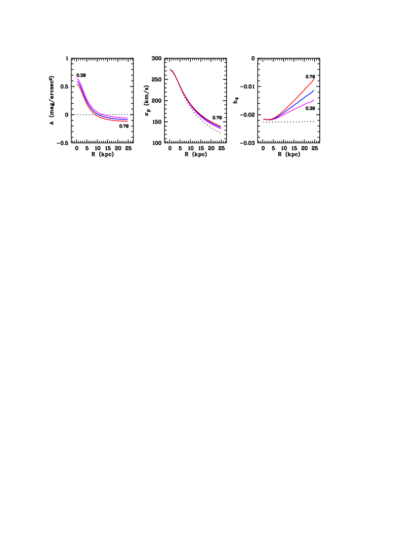
Figure 8: The effect of a dust albedo gradient on the attenuation curve and the observed kinematics, more precisely the projected dispersion and $h_{4}$ profiles. The adopted model is the isotropic template model in the $V$ band, but with a variable dust albedo of the form (19), with $\omega_{0}=\omega_{V}=0.59$, and three different values of $\omega_{\infty}$, being 0.79, 0.59 and 0.39. The black dotted curves correspond to the model without dust attenuation.

From the previously obtained results, we know that the effects of dust attenuation on the observed kinematics are due to photons emitted by high-velocity stars in the centre of the galaxy, scattered in the outer regions on lines of sight at large projected radii. The strength of these effects will hence depend on the probability that a photon from a high velocity star will be scattered onto outer lines of sight. There are various factors that can contribute to this probability. We already encountered two of them: the larger the dust content of the galaxy (high $\tau$) and/or the more extended the dust distributions (small $\alpha$), the greater the probability for scattering at large radii, and hence the stronger the effects on the observed kinematics. But also the optical properties of the dust can contribute to the number of scattering events that send photons from the inner lines of sight to outer lines of sight. Imagine, for example, that the scattering would be completely forward at large radii, or that the scattering albedo would become negligible in the outskirts of the galaxy. In either case, the probability that a photon emitted in the centre would reach the observer along a line of sight at large projected radii would be very small, such that the observed kinematics would hardly be affected by dust attenuation.

So far, we have adopted the assumption that the optical properties of the dust are equal all over the galaxy. However, this assumption might not always be satisfied in real elliptical galaxies. Indeed, gradients in e.g. the metallicity, the stellar radiation field or the X-ray luminosity density of a galaxy can cause systematic changes in the size distribution and/or chemical composition of the dust grains, which can result in gradients in their optical properties. In our own Galaxy, the physical properties of interstellar dust have been found to vary substantially in different environments (Witt, Bohlin & Stecher 1984; Mathis & Cardelli 1992).

With our Monte Carlo technique, we can easily include optical properties gradients in our models. The strongest effect can be expected for a gradient in the scattering albedo, because $\omega(r)$ is directly related to the number of scattering events at a distance $r$. We add to the template model of Section 4.3 an albedo gradient of the form

$$\omega(r)=\frac{\omega_{0}c^{2}+\omega_{\infty}r^{2}}{c^{2}+r^{2}},$$ (19)

which changes smoothly from $\omega_{0}$ in the centre to $\omega_{\infty}$ at large radii. In Fig. 8 we show the effect of such a gradient on the $\sigma_{p}$ and $h_{4}$ profiles, with the central albedo $\omega_{0}$ the value from Tab. 1, and a number of different values for $\omega_{\infty}$. This figure demonstrates that the attenuation effect on the observed kinematics becomes stronger for larger values of $\omega_{\infty}$, which agrees with the prediction that more scattering events correspond to a larger effect on the observed kinematics. Notice that for the reasonably large gradients in $\omega$ (more than 30 per cent), the differences between the various kinematical profiles are relatively small, and definitely within the observational errors.

6 Discussion

6.1 Dark matter halos around elliptical galaxies

In the outer regions of the galaxy, the observed kinematics are strongly affected by photons emitted in the central regions of the galaxy, that leave the galaxy after one or more scattering events along lines of sight with a large projected radius. Because these photons are emitted by stars that generally have larger velocities than the typical line-of-sight velocities appropriate along these lines of sight, they bias the LOSVDs towards larger velocities, and cause high-velocity wings. As a result, the projected velocity dispersion and the shape parameters $k_{4}$ and $h_{4}$ increase significantly at large projected radii.

These results are particularly important for the interpretation of the stellar kinematical evidence for dark matter halos around elliptical galaxies. For disc galaxies, the observational evidence for the existence of dark matter halos is convincing: the Hi rotation curves that remain flat or even rising out to very large radii, provide a clear proof of their existence (Freeman 1970; Faber & Gallagher 1979). For elliptical galaxies, this important tracer can generally not be used. A number of early-type galaxies, most of them classified as S0s, have neutral or ionized gas discs which can be used to estimate their dark matter content (Bertola et al. 1993; Franx et al. 1994), but these galaxies are exceptional cases and may not be representative for the general class of elliptical galaxies. The most convincing evidence for the existence of dark matter halos comes from measurements of the density and temperature of their hot X-ray emitting atmospheres (Forman, Jones & Tucker 1985; Matsushita et al. 1998; Loewenstein & White 1999), and from gravitational lensing (Griffiths et al. 1996; Keeton, Kochanek & Falco 1998). This evidence indicates that elliptical galaxies must have very large mass-to-light ratios at large radii, but, unfortunately, they do not contain much information about the detailed structure of a dark matter halo and its coupling to the luminous matter.

The most important way to trace dark matter halos around elliptical galaxies at small scales is by studying the stellar kinematics. With the present 8m class telescopes, stellar kinematics can be reliably traced out to several effective radii. If a dark matter halo is present, one expects the velocity dispersion profile to drop only slowly or to remain constant with projected radius. Such a behaviour was interpreted as a signature for the presence of a dark matter halo (Saglia, Bertin & Stiavelli 1992; Saglia et al. 1993). However, a slowly decreasing or nearly constant velocity dispersion profile can also be due to a strong tangential anisotropy at large radii. This so-called mass-anisotropy degeneracy (Gerhard 1993) can be broken by studying the LOSVD shape parameters: galaxies with a tangentially anisotropic orbital structure have a negative $h_{4}$. The combination of a slowly decreasing velocity dispersion profile and a positive $h_{4}$ at large projected radii, is generally interpreted as a indication of the presence of a dark matter halo. For a number of elliptical galaxies, the existence of dark halos has been advocated by such evidence (Rix et al. 1998; Gerhard et al. 1998; Kronawitter et al. 2000; Gerhard et al. 2001).

We show here that scattering off dust grains has the same effect on the dispersion profile as a dark halo: the dispersion will decrease more slowly than expected. Moreover, also the $h_{4}$ profiles are considerably biased towards larger values, such that the signature of an intrinsically tangential anisotropy can be weakened. Dust attenuation hence makes a foolproof detection of dark matter halos from stellar kinematical evidence much more complicated. It is obviously important to investigate to which degree dust can reduce or eliminate the need for a dark matter halo to explain the observed kinematics. Our first results indicate that a dust component that is shallower than the stars with $\tau_{V}=1$, has the same kinematic signature as a dark matter halo that contains half of the total mass of the galaxy (Baes & Dejonghe 2001c). An in-depth investigation of this topic, however, is beyond the scope of this paper, and a forthcoming paper will be devoted to this problem.

6.2 The determination of the dust distribution in elliptical galaxies

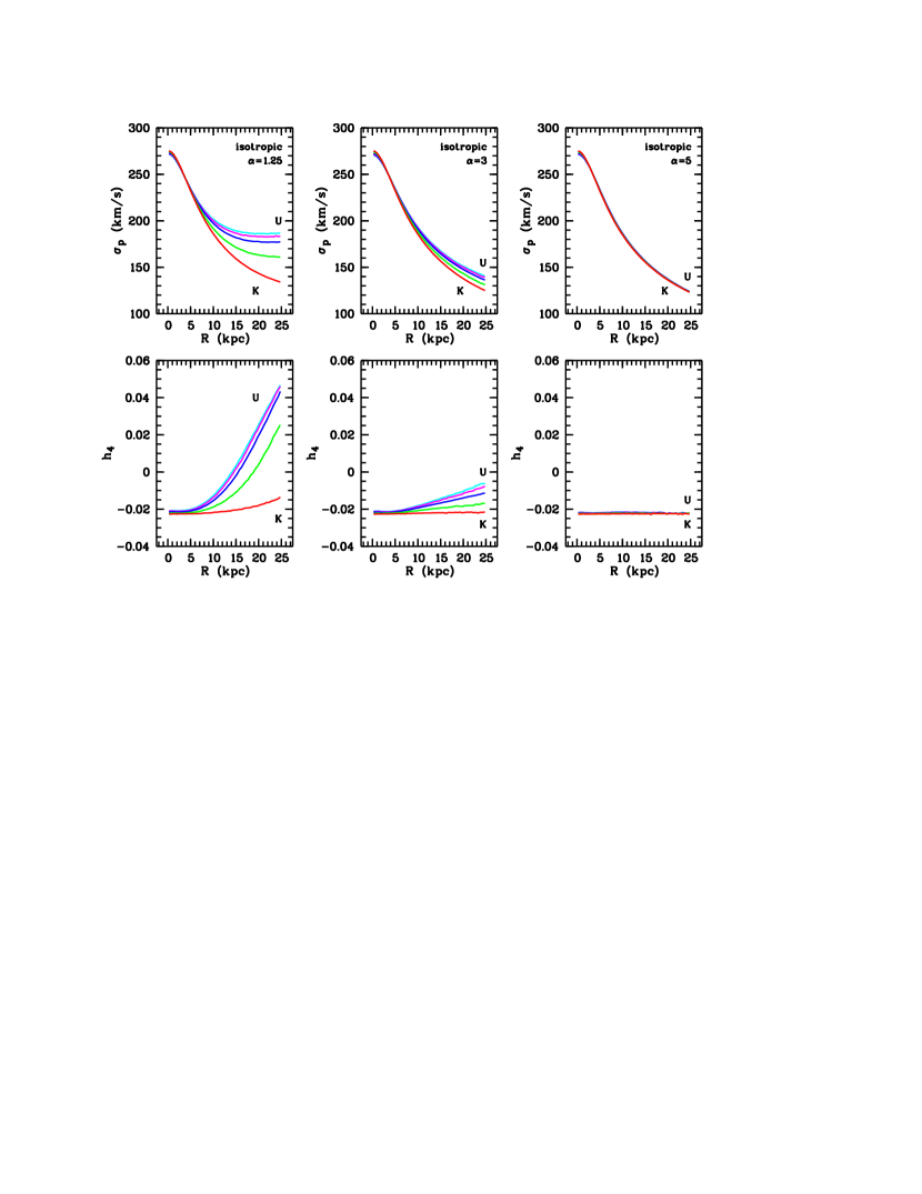
Figure 9: The observed kinematics in different colours as a tool to constrain the dust distribution in ellipticals. This figure shows how the projected velocity dispersion profile (upper panels) and the $h_{4}$ profile (lower panels) as they are observed in different wavebands. In each panel, the wavebands shown are the U, B, V, I, J and K bands. All models correspond to an isotropic Plummer model with a V-band optical depth $\tau_{V}=1$, but the three columns correspond to three different dust geometries: $\alpha=1.25$ (left), $\alpha=3$ (template model, middle) and $\alpha=5$ (right).

In the previous subsection, dust attenuation is considered as something troublesome or inconvenient – as an obstacle that prevents the observation of the true projected kinematics, and therefore complicates the interpretation of the true dynamical structure of elliptical galaxies. The fact that the observed kinematics are seriously affected by dust attenuation, can also serve in a more positive way: it can be used to trace the spatial distribution of the diffuse dust component in elliptical galaxies.

This is illustrated in Fig. 9, where we illustrate how the observed kinematics change with colour. The $\sigma_{p}$ and $h_{4}$ profiles in blue bands are more strongly affected by dust attenuation than those in red or near-infrared bands, because the extinction efficiency decreases with wavelength (Table 1). Combining this with the sensitive dependence of the observed kinematics on the dust geometry, we see that multi-colour kinematical profiles can help to constrain the spatial distribution of the dust. Indeed, if the dust is shallower than the stars ($\alpha$ small), the blue kinematics will be significantly affected by dust attenuation, whereas this effect will gradually become weaker if we look towards longer wavelengths. If, on the other hand, the dust has a similar distribution as the stars, the observed kinematics are hardly affected, even in blue colours, such that we will see no change of the kinematics with wavelength.

This method is also subject to a degeneration: differences between the stellar kinematics at different wavelengths can also be due to variations in the stellar populations, i.e. different absorption lines can trace different stellar types which do not necessarily need to be in the same dynamical state. The major problem, however, is the observational challenge: the projected kinematics need to be measured at different wavelengths with a sufficient accuracy out to several effective radii. Whereas this is nowadays possible in the optical, it is probably beyond the limit of the possibilities of the current generation of telescopes and instruments to do this at near-infrared wavelengths.

As a remark, we want to note that a similar principle has already been applied in another context: a number of authors have tried to constrain the dust content of disk galaxies by multi-wavelength analysis of the apparent rotation curves. Bosma et al. (1992) demonstrated how dust absorption can affect the observed rotation curve of edge-on spiral galaxies, and argued that the comparison of the optical and Hi rotation curves can be used as a new opacity test. Applying this test to the edge-on spiral galaxy NGC 891, they found that at least the outer regions of this galaxy must be optically thin. In a similar way, Prada et al. (1994) measured the ionized gas rotation curve of the inclined galaxy NGC 2146 at different wavelengths. They found a few discrepancies between the optical H$\alpha$ and the near-infrared [Siii] rotation curves in the center of the galaxy, which they could attribute to a dust lane, and a nice agreement between the rotation curves at large projected radii. Whence they concluded that NGC 2146 has to be largely transparent in its outer regions.

6.3 The central velocity dispersion in dusty galaxies

In Paper I, we found that the effects of absorption on the observed kinematics are only noticeable in the most central regions. For optical depths of order unity, absorption causes a decrease of the central dispersion with a few per cent. When scattering is taken into account, the effect of dust attenuation on the central dispersion is more complicated to predict. In particular, the nature (increase or decrease) and strength depend on the orbital structure of the galaxy. Although the magnitude of these effects is still modest (in particular compared to the effects of dust attenuation at large projected radii), this has some important implications.

A first area where the effects of dust attenuation should be taken into account are mass estimates. Indeed, the observed central velocity dispersion of galaxies is a parameter that is often adopted to quantify the total mass of a galaxy. For elliptical galaxies in the nearby universe, more accurate dynamical mass estimates are available through modelling of the entire observed kinematics. For other systems, however, in particular in the high-$z$ universe, the central velocity dispersion is often the only available kinematic property that can be measured with some reliability. The effects of dust attenuation can hence lead to a bias in simple mass estimates. Moreover, it is currently unclear how much dust is present in high-$z$ galaxies – a significant amount of dust production can be expected at the early epochs of star formation.

The central velocity dispersion also appears as an important parameter in the discussion about the presence and masses of black holes. It is believed that a significant fraction of the galaxies, if not all, harbour a massive black hole in their inner regions. The most reliable determination of the black hole masses in quiescent galaxies is by means of spatially resolved kinematics. This, however, represents a challenge for both observers and modellers, because it requires a very high spatial resolution and detailed dynamical modelling techniques. Mainly with high-resolution HST data, black hole masses have been determined for a number of nearby galaxies. It was found that they are tightly correlated with the central velocity dispersion of the host galaxies by a relationship $M_{\bullet}\propto\sigma^{a}$, with $a\approx 4$ (Gebhardt et al. 2000a; Ferrarese & Merritt 2000). Black hole masses of nearby AGNs, which can be determined by reverberation mapping (Blandford & McKee 1982; Kaspi et al. 2000), seem at first sight to satisfy this relation as well, albeit with some more scatter (Gebhardt et al. 2000b; Ferrarese et al. 2001). It is of course very tempting to adopt this relation for the determination of black hole masses in other galaxies, in particular at high $z$, where spatially resolved kinematics are beyond the present observational capabilities. However, because the lack of knowledge about the dust content of these galaxies, some caution is advised when applying this relation without taking attenuation effects into account.

6.4 Disk heating processes in spiral galaxies

It is generally known that the velocity dispersion of stars in the Galaxy increase with age (Wielen 1977). This is believed to be a result of the gradual heating of a initially cold disk due to irregularities in the gravitational potential. A number of possible scattering agents have been proposed for this heating, but the two most important mechanisms that contribute to this heating are thought to be scattering off giant molecular clouds (Spitzer & Schwarzschild 1951, 1953) and spiral density waves (Carlberg & Sellwood 1985). The study of the velocity ellipsoid in disk galaxies provides an interesting way to distinguish between these mechanisms, because each of them leaves a different kinematical signature. Spiral density waves are inefficient in scattering the stars in the vertical direction, such that it will result in a small $\sigma_{z}/\sigma_{R}$ ratio. On the other hand, molecular clouds tend to scatter stars rather isotropically, yielding an intermediate value for $\sigma_{z}/\sigma_{R}$. The axis ratio of the velocity ellipsoid is hence a very useful tool to identify the principal heating agent in spiral galaxies (Jenkins & Binney 1990; Merrifield, Gerssen & Kuijken 2001).

Unfortunately, the determination of the shape of the velocity ellipsoid in spirals is not straightforward. Gerssen, Kuijken & Merrifield (1997, 2000) showed that, in theory, it is possible to constrain the shape of the velocity ellipsoid of intermediately inclined spiral galaxies from the observed dispersion profiles on the major and minor axes.

From the results in this paper, however, we anticipate that dust attenuation has a strong effect on the projected dispersion profiles in disk galaxies, because of two reasons. First, disk galaxies contain large amounts of dust, typically several orders of magnitude larger than the average elliptical galaxy. The effects of attenuation are therefore likely too important to be considered as a second-order effect. Second, the differences in intrinsic velocity dispersion between bulge and disk are very large. If a photon, emitted by a high-velocity bulge star, propagates into the disk, and is scattered there such that it leaves the galaxy at a large projected radius, it will contribute a very large line-of-sight velocity to that LOSVD. A relatively small number of bulge star photons can therefore already seriously contaminate the LOSVDs and increase the observed projected dispersion at these lines of sight. Moreover, both the dust content and the bulge-disk ratio vary along the Hubble sequence, which definitely complicates a simple picture. These ideas definitely need a detailed investigation before major conclusions can be drawn on the heating processes in disk galaxies from the observed velocity ellipsoids.

7 Conclusions

The aim of this series of papers is to investigate the effects of a diffuse dust component on the observed kinematics of elliptical galaxies. We started in Paper I by investigating the effects of absorption only, neglecting the scattering effects. We found that, for realistic optical depths, these effects are modest, i.e. of the order of a few per cent in the central regions and completely negligible at larger projected radii.

In this paper, we extended our models to include the effects of scattering, which are usually considered as a second-order effect compared to absorption. The underlying thought is that the main effect of scattering is a reduction of the effects of absorption. It is therefore believed that the effects of scattering can be modelled by considering absorption with a reduced effective optical depth. From this point of view, it is often considered not worth the effort to properly include scattering in a proper way, thereby bypassing a costly radiative transfer treatment.

If we would have adopted this prescription, there would have been no reason to include scattering in our models. Indeed, because the effects of absorption only on the observed kinematics are already fairly small, the extra second-order effect of scattering should be completely negligible. However, a number of authors, foremost Witt et al. (1992), have shown that the effects of scattering are important, even for small optical depths, and that any way of neglecting or approximating them can lead to serious errors. We confirmed this in a previous study on the effects of dust attenuation on disk galaxies (Baes & Dejonghe 2001b).

In this paper, we have clearly demonstrated that, concerning the observed kinematics in elliptical galaxies, scattering can not be considered as a second-order effect to absorption. On the contrary, we find that the effects of dust attenuation are much more complicated and fascinating if scattering is included in the modelling. The way the kinematics of elliptical galaxies are affected can differ drastically, depending on which line of sight is considered, on the star-dust geometry and on the internal orbital structure of the galaxy. The most striking effect is the serious increase of both the velocity dispersion and the LOSVD shape parameters at large projected radii, due to photons from high-velocity stars scattered into the line of sight. This effect, which complicates the interpretation of the stellar kinematical evidence for dark matter halos around elliptical galaxies, has absolutely no counterpart when only absorption is taken into account. Results as these, which may seem unexpected at first sight, can be easily understood, once the idea of scattering as a second-order effect of absorption is abandoned.

Appendix A The spatial LOSVD for the Plummer model

A.1 The spatial LOSVD

The dynamical structure of a certain stellar population of a galaxy is completely determined by its phase space distribution function $F({\boldsymbol{r}},{\boldsymbol{v}})$. Whereas this function gives us, at a certain position in the galaxy, the three-dimensional distribution of the velocities, it is interesting from an observational point of view, interesting to know the (marginal) distribution of velocities into an arbitrary direction ${\boldsymbol{k}}$, for example the direction towards the observer. To calculate this distribution, we construct a new cartesian reference system $({\boldsymbol{e}}_{\perp_{1}},{\boldsymbol{e}}_{\perp_{2}},{\boldsymbol{e}}_{\parallel})$, such that ${\boldsymbol{k}}={\boldsymbol{e}}_{\parallel}$. The spatial LOSVD $\phi({\boldsymbol{r}},{\boldsymbol{k}},v_{\parallel})$ is defined through the relation

$$\ell({\boldsymbol{r}})\,\phi({\boldsymbol{r}},{\boldsymbol{k}},v_{\parallel})={\mathcal{L}}\iint F({\boldsymbol{r}},{\boldsymbol{v}})\,{\text{d}}v_{\perp_{1}}\,{\text{d}}v_{\perp_{2}}.$$ (20)

The emissivity is taken into this definition in order to have the normalization

$$\int\phi({\boldsymbol{r}},{\boldsymbol{k}},v_{\parallel})\,{\text{d}}v_{\parallel}=\frac{\mathcal{L}}{\ell({\boldsymbol{r}})}\iiint F({\boldsymbol{r}},{\boldsymbol{v}})\,{\text{d}}{\boldsymbol{v}}=1.$$ (21)

The spatial LOSVD hence represents the probability for a star at a position ${\boldsymbol{r}}$, to have a velocity component $v_{\parallel}$ in the direction ${\boldsymbol{k}}$. The quantity $\ell({\boldsymbol{r}})\,\phi({\boldsymbol{r}},{\boldsymbol{k}},v_{\parallel})$ then represents the stellar emissivity at ${\boldsymbol{r}}$ of stars which have a velocity $v_{\parallel}$ in the direction ${\boldsymbol{k}}$.

For the calculation of the spatial LOSVD, it is important to know that a distribution function will not depend on the six phase space coordinates $({\boldsymbol{r}},{\boldsymbol{v}})$ independently, but only through a number of integrals of motion. In a spherical galaxy, we can write the distribution function generally as $F(E,L)$, where $E$ and $L$ are the binding energy and angular momentum integrals respectively (Binney & Tremaine 1987). Because the distribution function only depends on $v_{\theta}$ and $v_{\phi}$ through the combination $v_{T}^{2}=v_{\theta}^{2}+v_{\phi}^{2}$, we can choose our reference system such that ${\boldsymbol{e}}_{\perp_{2}}={\boldsymbol{e}}_{\theta}$. If we denote the angle between ${\boldsymbol{k}}$ and ${\boldsymbol{e}}_{r}$ as $\eta$, we then find

$$E=\psi(r)-\tfrac{1}{2}v_{\perp_{1}}^{2}-\tfrac{1}{2}v_{\perp_{2}}^{2}-\tfrac{1}{2}v_{\parallel}^{2}$$ (22)

$$L^{2}=r^{2}\,\left(v_{\perp_{1}}^{2}\cos^{2}\eta+v_{\perp_{2}}^{2}+v_{\parallel}^{2}\sin^{2}\eta-v_{\perp_{1}}\,v_{\parallel}\sin 2\eta\right).$$ (23)

Substitution of these expressions into the distribution function allows in principle to calculate the spatial LOSVD using expression (20).

A.2 The Plummer model

A major advantage of the Plummer model is it allows the construction of a completely analytical one-parameter family of self-consistent dynamical models (Dejonghe 1987). The different models are characterized by a parameter $q$, restricted by $q\leqslant 2$. This parameter is determines the orbital structure of the galaxy: negative values of $q$ correspond to a tangential anisotropy, positive values to a radial anisotropy, whereas for $q=0$ the model is isotropic. By means of Laplace-Mellin transforms the corresponding distribution function $F(E,L)$ can be calculated analytically for all values of $q$ (Dejonghe 1986). For general values of $q$, the distribution function can be expressed in terms of hypergeometric functions. For even integer values of $q$ however, the distribution function becomes much simpler, which will allow us to calculate the spatial LOSVD explicitly.

A.2.1 The isotropic model $q=0$

For the isotropic dynamical models, the distribution funciton is only function of the binding energy. For the Plummer model, it is a simple power law of $E$,

$$F(E)=\frac{3}{7\pi^{3}}\,\frac{1}{c^{3}u^{3}}\,\left(\frac{2E}{u^{2}}\right)^{7/2},$$ (24)

where $u=\sqrt{GM/c}$ represents a characteristic velocity. Substituting the distribution function (24) into the definition (20), we obtain, using the expression (22),

$$\phi({\boldsymbol{r}},{\boldsymbol{k}},v_{\parallel})=\frac{256}{63\pi}\,\frac{1}{\sqrt{2\psi(r)}}\,\left[1-\frac{v_{\parallel}^{2}}{2\psi(r)}\right]^{9/2}.$$ (25)

Because the distribution function of isotropic galaxies is completely symmetric in the three velocity components, the spatial LOSVD is independent of the direction ${\boldsymbol{k}}$. It is straightforward to check that the normalization condition (21) is satisfied.

A.2.2 The radial model $q=2$

For $q=2$, the most radial model in the Plummer family, the distribution function vanishes for $2E\leqslant L^{2}/c^{2}$, whereas reduces to a simple form for $2E\geqslant L^{2}/c^{2}$,

$$F(E,L)=\frac{3}{4\pi^{3}}\,\frac{1}{c^{3}u^{5}}\left(2E-\frac{L^{2}}{c^{2}}\right)^{3/2}.$$ (26)

To calculate the spatial LOSVD, one has to substitute the expressions (22) and (23) into this distribution function, and integrate it with respect to $v_{\perp_{1}}$ and $v_{\perp_{2}}$, where the integration surface in determined by the condition $2E\geqslant L^{2}/c^{2}$. After some algebra, one finds that the LOSVD is given by

$$\phi({\boldsymbol{r}},{\boldsymbol{k}},v_{\parallel})=\frac{16}{5\pi}\,\frac{1}{\sqrt{2A\psi(r)}}\,\left[1-\frac{v_{\parallel}^{2}}{2A\psi(r)}\right]^{5/2},$$ (27)

for $|v_{\parallel}|\geqslant\sqrt{2A\psi(r)}$, with

$$A=\frac{r^{2}\cos^{2}\eta+c^{2}}{r^{2}+c^{2}}\leqslant 1.$$ (28)

The normalization condition (21) can be easily checked.

A.2.3 Tangential models with $q=-2m$

For general negative values of $q$, the Plummer distribution function can be written in terms of hypergeometric series. If $q$ is a negative even integer, $q=-2m$, this series breaks down after a finite number of terms, and the distribution function then becomes a finite series, where each term is a power law of $E$ and $L$ (Dejonghe 1986). The spatial LOSVD can be calculated for each of these distribution functions following the same recipe as for the radial $q=2$ model. An alternative, elegant way to calculate the spatial LOSVDs for these models using Laplace transforms is presented by De Rijcke (2000). After lengthy calculations, one finds eventually

$$\phi({\boldsymbol{r}},{\boldsymbol{k}},v_{\parallel})=\frac{1}{\sqrt{\pi}}\,\frac{\Gamma(6+2m)}{\Gamma\left(\frac{11}{2}+2m\right)}\,\frac{1}{\sqrt{2\psi(r)}}\,\left[1-\frac{v_{\parallel}^{2}}{2\psi(r)}\right]^{\frac{9}{2}+2m}\\ \times\sum_{j=0}^{m}\frac{\left(\tfrac{1}{2}\right)_{j}\left(-m\right)_{j}}{(j!)^{2}}\left(\frac{r^{2}\sin^{2}\eta}{r^{2}+c^{2}}\right)^{2j}\left[1-\frac{v_{\parallel}^{2}}{2\psi(r)}\right]^{-j}\,\\ \times{}_{2}F_{1}\left(-j,5+2m;\tfrac{1}{2};\frac{v_{\parallel}^{2}}{2\psi(r)}\right),$$ (29)

where $(a)_{j}$ represents the Pochammer symbol

$$(a)_{j}=a(a+1)(a+2)\cdots(a+j-1).$$ (30)

Setting $q=m=0$ in the expression (29), it reduces to the expression (25) we found for the isotropic Plummer galaxy. To check the normalization of the spatial LOSVDs we have to evaluate the integral

$${\mathcal{I}}(m,j)=\int_{0}^{1}(1-x^{2})^{\frac{9}{2}+2m-j}{}_{2}F_{1}(-j,2m+5;\tfrac{1}{2};x^{2})\,{\text{d}}x,$$ (31)

for all $j\leqslant m$. By means of formula (7.512.4) of Gradshteyn & Ryzhik (1965) we find that this integral vanishes for $j>0$, whereas for $j=0$ we obtain

$${\mathcal{I}}(m,0)=\frac{\sqrt{\pi}}{2}\,\dfrac{\Gamma\left(\tfrac{11}{2}+2m\right)}{\Gamma(6+2m)}.$$ (32)

Only the first term in the summation in equation (29) will hence contribute to the integral over $v_{\parallel}$, and it is obvious that the final result will equal 1.

Appendix B Anisotropic scattering and the importance of the dust grain velocity terms in equation (10)

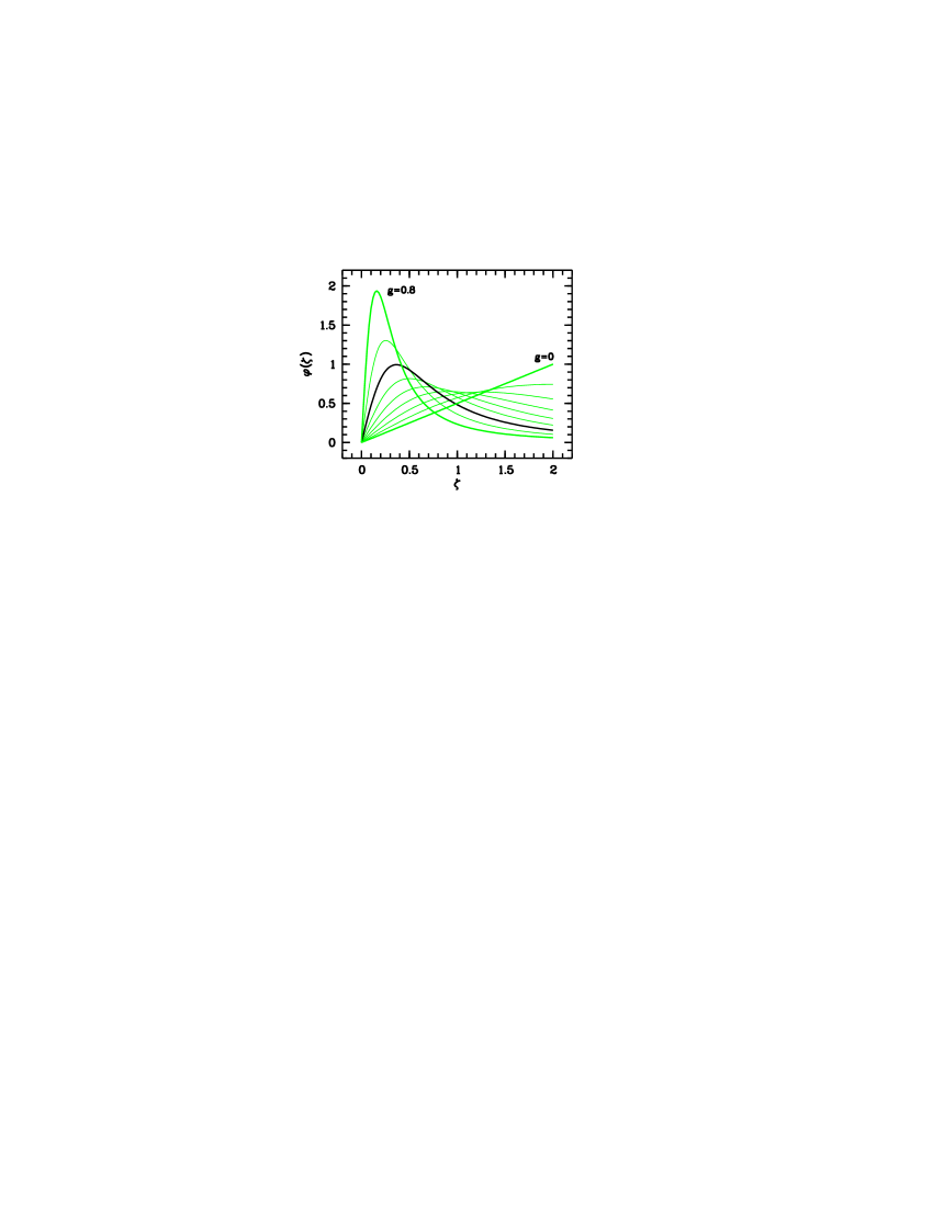
Figure 10: The probability density $\varphi(\zeta)$ for $\zeta\equiv\|{\boldsymbol{k}}_{i}-{\boldsymbol{k}}_{i-1}\|$, corresponding to the Henyey-Greenstein phase function. Curves are shown for different values of the asymmetry parameter $g$, ranging between $g=0$ and $g=0.8$, in steps of 0.1. The black lines indicates the probability density for $g=0.6$, appropriate for the optical regime.

Table 2: The mean, the median and the maximum value for the probability density $\varphi(\zeta)$ corresponding to the Henyey-Greenstein phase function, for different values of the anisotropy parameter $g$.

$g$	$\zeta_{\text{mean}}$	$\zeta_{\text{med}}$	$\zeta_{\text{peak}}$
0.0	1.33	1.41	2.00
0.1	1.25	1.30	2.00
0.2	1.16	1.19	1.26
0.3	1.07	1.06	0.90
0.4	0.98	0.93	0.67
0.5	0.87	0.79	0.50
0.6	0.75	0.64	0.37
0.7	0.63	0.49	0.25
0.8	0.48	0.33	0.16
0.9	0.29	0.17	0.07
1.0	0.00	0.00	0.00

Each term in the summation in expression (10) is a inner product of the velocity vector ${\boldsymbol{v}}_{d_{i}}$ and the relative direction vector ${\boldsymbol{k}}_{i}-{\boldsymbol{k}}_{i-1}$. It is obvious that the contribution of one such term does not depend only on the dust grain velocity $v_{d_{i}}$, but also on the scattering angle. The distribution of scattering angles will therefore also play a role in the importance of the dust grain velocity terms in equation (10). If, for example, the propagation direction of a photon is on average only slightly changed during a scattering event, we find that ${\boldsymbol{k}}_{i}\approx{\boldsymbol{k}}_{i-1}$, which reduces the magnitude of the dust grains velocity terms.

We can illustrate this nicely by calculating the statistical distribution of the modulus of the vector ${\boldsymbol{k}}_{i}-{\boldsymbol{k}}_{i-1}$, i.e. we will calculate the probability density $\varphi(\zeta)$ for $\zeta\equiv\|{\boldsymbol{k}}_{i}-{\boldsymbol{k}}_{i-1}\|$. Since the directions ${\boldsymbol{k}}_{i-1}$ and ${\boldsymbol{k}}_{i}$ represent unit vectors, elementary trigonometry learns that

$$\zeta=\sqrt{2(1-\cos\alpha)},$$ (33)

where $\alpha$ is the scattering angle. The scattering angle is distributed according to the phase function $\Phi(\cos\alpha)$, such that

$$\varphi(\zeta)=\tfrac{1}{2}\,\Phi\left(1-\tfrac{\zeta^{2}}{2}\right)\,\zeta,$$ (34)

with $\zeta$ taking values between 0 and 2. If the scattering is isotropic, the phase function has the simple form $\Phi(\cos\alpha)=1$, such that $\varphi(\zeta)=\zeta/2$. Larger values for $\zeta$ will hence be preferred. If we adopt Henyey-Greenstein scattering (see Section 4.2.2), we can calculate the corresponding values for different degrees of anisotropy. In Fig. 10, the probability density $\varphi(\zeta)$ corresponding to the Henyey-Greenstein phase function (17) is shown for different values of anisotropy parameters $g$. In the limit $g=0$, this function of course reduces to the isotropic equivalent $\varphi(\zeta)=\zeta/2$. If the anisotropy parameter increases, however, smaller values for $\zeta$ will gradually become dominant. We can quantify this trend by calculating the mean value $\zeta_{\text{mean}}$, the median $\zeta_{\text{med}}$ or the value $\zeta_{\text{peak}}$ for which $\varphi(\zeta)$ reaches its maximum value. For the isotropic phase function we find $\zeta_{\text{mean}}=\tfrac{4}{3}$, $\zeta_{\text{med}}=\sqrt{2}$ and $\zeta_{\text{peak}}=2$, whereas for the Henyey-Greenstein phase function, we obtain

$$\zeta_{\text{mean}}=\frac{1-g}{g}\left[\frac{1+g}{\sqrt{g}}\,\ln\left(\frac{1+\sqrt{g}}{\sqrt{1-g}}\right)-1\right]$$ (35)

$$\zeta_{\text{med}}=\sqrt{g^{3}-3g+2}$$ (36)

$$\zeta_{\text{peak}}=\min\left(2,\frac{1-g}{\sqrt{2g}}\right).$$ (37)

In Table 2 we tabulate $\zeta_{\text{mean}}$, $\zeta_{\text{med}}$ and $\zeta_{\text{peak}}$ as a function of the asymmetry parameter. This table confirms that smaller values of $\zeta$ quickly start to dominate as $g$ grows larger. In particular, for the anisotropy parameters appropriate in the optical regime, $g\sim 0.6$ (see Table 1), the density $\varphi(\zeta)$ clearly favours fairly small values for $\zeta$ (black curve in Fig. 10). As a consequence, $\|{\boldsymbol{k}}_{i}-{\boldsymbol{k}}_{i-1}\|$ will be fairly small in the majority of the scattering events. The anisotropic nature of scattering hence contributes to reducing the importance of the dust grain velocity terms in equation (10).

References

- [1] Abramowitz M., Stegun I. A., 1972, Handbook of Mathematical Functions. Dover Publications Inc., New York
- [2] Baes M., Dejonghe H., 2000, MNRAS, 313, 153 [paper I]
- [3] Baes M., Dejonghe H., 2001a, MNRAS, 326, 722
- [4] Baes M., Dejonghe H., 2001b, MNRAS, 326, 733
- [5] Baes M., Dejonghe H., 2001c, ApJ, 563, L19
- [6] Baes M., Dejonghe H., De Rijcke S., 2000, MNRAS, 318, 798 [paper II]
- [7] Bally J., Thronson H. A., 1989, AJ, 97, 69
- [8] Bertola F., Pizzella A., Persic M., Salucci P., 1993, ApJ, 416, L45
- [9] Bianchi S., Ferrara A., Giovanardi C., 1996, ApJ, 465, 127
- [10] Bianchi S., Davies J. I., Alton P. B., 2000, A&A, 359, 65
- [11] Bianchi S., Ferrara A., Davies J. I., Alton P. B., 2000, MNRAS, 311, 601
- [12] Binney J., Tremaine S., 1987, Galactic Dynamics. Princeton Univ. Press, Princeton
- [13] Blandford R. D., McKee C. F., 1982, ApJ, 255, 419
- [14] Bosma A., Byun Y., Freeman K. C., Athanassoula E., 1992, ApJ, 400, L21
- [15] Carlberg R. G., Sellwood J. A., 1985, ApJ, 292, 79
- [16] Cashwell E. D., Everett C. J., 1959, A Practical Manual on the Monte Carlo Method for Random Walk Problems. Pergamon, New York
- [17] Chandrasekhar S., 1934, MNRAS, 94, 444
- [18] Chandrasekhar S., 1960, Radiative Transfer, Dover Publications, New York
- [19] Code A. D., Whitney B. A., 1995, ApJ, 441, 400
- [20] Dejonghe H., 1986, Phys. Rep., 133, 217
- [21] Dejonghe H., 1987, MNRAS, 224, 13
- [22] Dejonghe H., 1989, ApJ, 343, 113
- [23] De Rijcke S., 2000, PhD Thesis, Univ. Gent
- [24] Di Bartolomeo A., Barbaro G., Perinotto M., 1995, MNRAS, 277, 1279
- [25] Disney M. J., Davies J. I., Phillips S., 1989, MNRAS, 239, 939
- [26] Ebneter K., Balick B., 1985, AJ, 90, 183
- [27] Faber S. M., Gallagher J. S., 1979, ARA&A, 17, 135
- [28] Freeman K. C., 1970, ApJ, 160, 811
- [29] Ferrarese L., Merritt D., 2000, ApJ, 539, L9
- [30] Ferrarese L., Pogge R. W., Peterson B. M., Merritt D., Wandel A., Joseph C. L., 2001, ApJ, 555, L79
- [31] Ferrari F., Pastoriza M. G., Macchetto F., Caon N., 1999, A&AS, 136, 269
- [32] Fich M., Hodge P., 1993, ApJ, 415, 75
- [33] Fischer O., Henning Th., Yorke H. W., 1994, A&A, 284, 187
- [34] Flannery B. P., Roberge W., Rybicki G. B., 1980, ApJ, 236, 598
- [35] Forman W., Jones C., Tucker W., 1985, ApJ, 293, 102
- [36] Franx M., van Gorkom J., de Zeeuw T., 1994, ApJ, 293, 102
- [37] Gebhardt K., Bender R., Bower G., Dressler A., Faber S. M., Filippenko A. V., Green R., Grillmair C., Ho L. C., Kormendy J., Lauer T. R., Magorrian J., Pinkney J., Richstone D., Tremaine S., 2000a, ApJ, 539, L13
- [38] Gebhardt K., Kormendy J., Ho L. C., Bender R., Bower G., Dressler A., Faber S. M., Filippenko A. V., Green R., Grillmair C., Lauer T. R., Magorrian J., Pinkney J., Richstone D., Tremaine S., 2000b, ApJ, 543, 5
- [39] Gerhard O. E., 1993, MNRAS, 265, 213
- [40] Gerhard O., Jeske G., Saglia R. P., Bender R., 1998, MNRAS, 295, 197
- [41] Gerhard O., Kronawitter A., Saglia R. P., Bender R., 2001, AJ, 121, 1936
- [42] Gerssen J., Kuijken K., Merrifield M. R., 1997, MNRAS, 288, 618
- [43] Gerssen J., Kuijken K., Merrifield M. R., 2000, MNRAS, 317, 545
- [44] Gradshteyn I. S., Ryzhik I. M., 1965, Table of Integrals, Series and Products. Academic Press Inc., New York
- [45] Griffiths R. E., Casertano S., Im M., Ratnatunga K. U., 1996, MNRAS, 282, 1159
- [46] Gordon K. D., Calzetti D., Witt A. N., 1997, ApJ, 487, 625
- [47] Gordon K. D., Misselt K. A., Witt A. N., Clayton G. C., 2001, ApJ, 551, 269
- [48] Goudfrooij P., de Jong T., 1995, A&A, 298, 784
- [49] Gros M., Crivellari L., Simonneau E., 1997, ApJ, 489, 311
- [50] Hawarden T. G., Elson R. A. W., Longmore A. J., Tritton S. B., Corwin H. G. Jr., 1981, MNRAS, 196, 747
- [51] Hummer D. G., Rybicki G. B., 1971, MNRAS, 152, 1
- [52] Jenkins A., Binney J., 1990, MNRAS, 245, 305
- [53] Jura M., 1986, ApJ, 306, 483
- [54] Kaspi S., Smith P. S., Netzer H., Maoz D., Jannuzi B. T., Giveon U., 2000, ApJ, 533, 631
- [55] Knapp G. R., Gunn J. E., Wynn-Williams C. G., 1992, ApJ, 399, 76
- [56] Keeton C. R., Kochanek C. S., Falco E. E., 1998, ApJ, 509, 561
- [57] Kosirev N. A., 1934, MNRAS, 94, 430
- [58] Kronawitter A., Saglia R. P., Gerhard O., Bender R., 2000, A&AS, 144, 53
- [59] Leeuw L. L., Sansom A. E., Robson E., 2000, MNRAS, 311, 683
- [60] Loewenstein M., White R. E. III, 1999, ApJ, 518, 50
- [61] Mathis J. S., Cardelli J. A., 1992, ApJ, 398, 610
- [62] Matsushita K., Makishima K., Ikebe Y., Rokutanda E., Yamasaki N., Ohashi T., 1998, ApJ, 499, L13
- [63] Mattila K., 1970, A&A, 9, 53
- [64] Matthews L., Wood K., 2001, ApJ, 548, 150
- [65] Merluzzi P., 1998, A&A, 338, 807
- [66] Merrifield M., Gerssen J., Kuijken K., 2001, in Galaxy Disks and Disk Galaxies, J. G. Funes S. J. and E. M. Corsini eds., ASP Conf. Series, 230, 221
- [67] Michard R., 2000, A&A, 360, 85
- [68] Mihalas D., 1978, Stellar Atmospheres, W. H. Freeman and Co., San Francisco
- [69] Misselt K. A., Gordon K. D., Clayton G. C., Wolff M. J., 2001, ApJ, 551, 277
- [70] Peraiah A., Varghese B. A., 1985, ApJ, 290, 411
- [71] Plummer H. C., 1911, MNRAS, 71, 460
- [72] Prada F., Beckman J. E., McKeith C. D., Castles J., Greve A., 1994, ApJ, 423, L35
- [73] Press W. H., Flannery B. P., Teukolsky S. A., Vetterling W. T., 1989, Numerical Recipes. Cambridge Univ. Press, Cambridge
- [74] Rix H.-W. de Zeeuw P. T., Cretton N., van der Marel R. P., Carollo C. M., 1997, ApJ, 488, 702
- [75] Rogers C., Martin P. G., 1984, ApJ, 284, 327
- [76] Rowan-Robinson M., 1980, ApJS, 44, 403
- [77] Saglia R. P., Bertin G., Stiavelli M., 1992, ApJ, 384, 433
- [78] Saglia R. P., Bertin G., Bertola F., Danziger J., Dejonghe H., Sadler E. M., Stiavelli M., de Zeeuw P. T., Zeilinger W. W., 1993, ApJ, 403, 567
- [79] Schmid-Burgk J., 1975, A&A, 40, 249
- [80] Spitzer L. Jr., Schwarzschild M., 1951, ApJ, 114, 385
- [81] Spitzer L. Jr., Schwarzschild M., 1953, ApJ, 118, 106
- [82] Tomita A., Aoki K., Watanabe M., Takata T., Ichikawa S., 2000, AJ, 120, 123
- [83] Tran H. D., Tsvetanov Z., Ford H. C., Davies J., Jaffe W., van den Bosch F. C., Rest A., 2001, AJ, 121, 2928
- [84] van der Marel R. P., Franx M., 1993, ApJ, 407, 525
- [85] van Dokkum P. G., Franx M., 1995, AJ, 110, 2027
- [86] Véron-Cetty M.-P., Véron P., 1988, A&A, 204, 28
- [87] Wielen R., 1977, A&A, 60, 263
- [88] Wiklind T., Henkel C., 1995, A&A, 297, L71
- [89] Wise M. S., Silva D. R., 1996, ApJ, 461, 155
- [90] Witt A. N., 1977, ApJS, 35, 1
- [91] Witt A. N., Gordon K. D., 1996, ApJ, 463, 681
- [92] Witt A. N., Bohlin R. C., Stecher T. P., 1984, ApJ, 279, 698
- [93] Witt A. N., Thronson H. A. Jr., Capuano J. M. Jr., 1992, ApJ, 393, 611
- [94] Wolf S., Fischer O., Pfau W., 1998, A&A, 340, 103
- [95] Wolf S., Henning Th., Stecklum B., 1999, A&A, 349, 839
- [96] Wood K., Reynolds R. J., 1999, ApJ, 525, 799
- [97] Wybo M., Dejonghe H., 1996, A&A, 312, 649
- [98] Yorke H. W., 1980, A&A, 86, 286
- [99] Yusef-Zadeh F., Morris M., White R. L., 1984, ApJ, 278, 186