Perturbation theory in Lagrangian hydrodynamics for a cosmological fluid with velocity dispersion

Abstract

We extensively develop a perturbation theory for nonlinear cosmological dynamics, based on the Lagrangian description of hydrodynamics. We solve hydrodynamic equations for a self-gravitating fluid with pressure, given by a polytropic equation of state, using a perturbation method up to second order. This perturbative approach is an extension of the usual Lagrangian perturbation theory for a pressureless fluid, in view of inclusion of the pressure effect, which should be taken into account on the occurrence of velocity dispersion. We obtain the first-order solutions in generic background universes and the second-order solutions in wider range of a polytropic index, whereas our previous work gives the first-order solutions only in the Einstein-de Sitter background and the second-order solutions for the polytropic index $4/3$. Using the perturbation solutions, we present illustrative examples of our formulation in one- and two-dimensional systems, and discuss how the evolution of inhomogeneities changes for the variation of the polytropic index.

I Introduction

Hydrodynamics is a powerful tool to study various astrophysical phenomena, from those associated with compact objects up to large-scale structure formation. For example, when investigating gravitational instability of cold dark matter for structure formation, analyses are easier to handle by adopting a hydrodynamical description, rather than by trying to solve the Boltzmann equation of a self-gravitating N-particles system. The linear perturbation theory of a homogeneous and isotropic universe weinberg ; peebles ; pad ; coles ; saco is a typical case, which gives a qualitative estimate for gravitational instability. It is based on the Eulerian picture of hydrodynamics, while approximations based on the Lagrangian hydrodynamics has been recognized to be more useful, such as the celebrated Zel’dovich approximation zel ; buchert92 ; munshi . This paper deals with an approximation theory of gravitational instability based on the Lagrangian hydrodynamics.

Although the Zel’dovich approximation has been found to give an accurate description up to the stage where density perturbations grow to be unity, it involves a serious shortcoming that it cannot be applied after caustics in the density field are formed. In the Zel’dovich approximation, the fluid elements continue to move in the directions that are determined by initial conditions all the time, and consequently high density regions such as ‘pancakes’ cannot stay compact beyond the caustic formation, while numerical simulations have shown the presence of clumps with a very wide range in mass at any given time davis . Moreover, once caustics in the density field are formed, a hydrodynamical description itself is not valid in general. Then, do we have to abandon a hydrodynamical description and try to solve the Boltzmann equation, or tackle N-body simulations?

In order to proceed with a hydrodynamical description without the formation of caustics, the ‘adhesion approximation’ gurbatov has been proposed, in which an artificial viscosity term is added to the Zel’dovich approximation. This modified approximation successfully describes the stage where the original Zel’dovich approximation breaks down, but the physical origin of the viscosity term should be clarified. Some remarkable works have been done on this issue; Buchert and Domínguez budo argued, by beginning with the collisionless Boltzmann equation BT , that the effect of velocity dispersion become important beyond the caustics, where multi-stream flow arises, and the presence of velocity dispersion of the flow can yield pressure-like or viscosity terms; Buchert et al. bdp showed how the viscosity term is generated by a pressure-like force of a fluid under the assumptions that the peculiar acceleration is parallel to the peculiar velocity; Domínguez domi00 clarified that a hydrodynamic formulation is achieved via a spatial coarse graining in a many-body gravitating system, and the ‘adhesion approximation’ can be derived by the expansion of coarse-grained equations with respect to the smoothing length. (See also Ref. domi0106 .) In these works, they also obtained implications for an ‘equation of state’, which is a phenomenological relationship between kinematical pressure $P$ and mass density $\rho$. Buchert and Domínguez budo found that, if the effect of velocity dispersion is small and the velocity dispersion is approximately isotropic, the equation of state should take the form $P\propto\rho^{5/3}$; Buchert et al. bdp showed that an adhesion-like equation can be derived if the equation of state is assumed as $P\propto\rho^{2}$; Moreover, a plausible value of the polytropic index $\gamma\equiv{\rm d}\ln P/{\rm d}\ln\rho$ has been found to be close to $5/3$ from cosmological N-body simulations domi0103 .

From these aspects, it is of interest to extend a Lagrangian perturbation scheme to a fluid with pressure, and to explore how the scheme works as an approximation for cosmological structure formation. Actually, Adler and Buchert adler and Morita and Tatekawa moritate have formulated perturbation theory in the Lagrangian hydrodynamics, taking into account the pressure effect under the assumption that the pressure is a function of the mass density only. In our earlier work moritate , imposing a polytropic relation as the equation of state, we solved the Lagrangian perturbation equations up to second order for cases where the equations are solved easily, and showed illustrative examples with the solutions in a one-dimensional system. In particular, the second-order solutions were obtained only for the case in which the polytropic index $\gamma$ is $4/3$, while a plausible value of $\gamma$ seems to be larger, as was mentioned above.

In this paper, we extend our earlier work by solving the first-order perturbation equations in generic background universes and the second-order perturbation equations for wider range of a polytropic index, and by presenting illustrations in one- and two-dimensional systems. We examine how the behavior of the perturbation solutions, and the resultant evolution of inhomogeneities, change for the variation of the polytropic index. This enables us to discuss whether, or for what kind of the equation of state, the adhesion-type approximation is realized in the Lagrangian perturbation scheme.

This paper is organized as follows. In Sec. II, we present Lagrangian hydrodynamic equations, governing the system we consider. In Sec. III, the first-order perturbation equations are derived and their solutions are shown, not only in the Einstein-de Sitter background but also in more generic backgrounds. In Sec. IV, we obtain the second-order perturbation equations and present their solutions in an approximate form for $\gamma>4/3$. Section V provides illustrative examples of our formulation in one- and two-dimensional models. In Sec. VI, we discuss our results and state our conclusions.

II Basic equations

In this section, we present hydrodynamic equations in the Lagrangian description, which our approach stands on. The matter model we consider is a self-gravitating fluid with energy density $\rho$ and pressure $P$, which arises in the presence of velocity dispersion. Then the basic equations we start from are

$$\frac{\partial\rho}{\partial t}+3\frac{\dot{a}}{a}\rho+\frac{1}{a}\nabla_{\bm{x}}\cdot(\rho\bm{v})=0\,,$$ (1)

$$\frac{\partial\bm{v}}{\partial t}+\frac{\dot{a}}{a}\bm{v}+\frac{1}{a}(\bm{v}\cdot\nabla_{\bm{x}})\bm{v}=\bm{g}-\frac{1}{\rho a}\nabla_{\bm{x}}P\,,$$ (2)

$$\nabla_{\bm{x}}\times\bm{g}=0\,,$$ (3)

$$\nabla_{\bm{x}}\cdot\bm{g}=-4\pi Ga(\rho-\rho_{\rm b})\,,$$ (4)

where $\bm{v}$ and $\bm{g}$ are the peculiar velocity and the peculiar gravitational field, respectively, which represent the deviation from a background, homogeneous and isotropic universe. The cosmic scale factor $a(t)$ and the energy density $\rho_{\rm b}(t)$ of the background universe satisfy the Friedmann equations

$$\left(\frac{\dot{a}}{a}\right)^{2} = \frac{8\pi G}{3}\rho_{\rm b}-\frac{\mathcal{K}}{a^{2}}+\frac{\Lambda}{3}\,,$$ (5)

$$\frac{\ddot{a}}{a} = -\frac{4\pi G}{3}\rho_{\rm b}+\frac{\Lambda}{3}\,,$$ (6)

with a curvature constant $\mathcal{K}$ and a cosmological constant $\Lambda$. In order to solve the hydrodynamic equations, we must specify an equation of state. Throughout this paper, we consider barotropic fluids, in which the pressure $P$ is a function of the energy density only, $P=P(\rho)$.

Introducing the Lagrangian time derivative

$$\frac{\rm d}{{\rm d}t}\equiv\frac{\partial}{\partial t}+\frac{1}{a}(\bm{v}\cdot\nabla_{\bm{x}})\,,$$

Eqs. (1) and (2) become

$$\frac{{\rm d}\rho}{{\rm d}t}+3\frac{\dot{a}}{a}\rho+\frac{\rho}{a}(\nabla_{\bm{x}}\cdot\bm{v})=0\,,$$ (7)

$$\frac{{\rm d}\bm{v}}{{\rm d}t}+\frac{\dot{a}}{a}\bm{v}=\bm{g}-\frac{1}{\rho a}\nabla_{\bm{x}}P\,.$$ (8)

In the Lagrangian hydrodynamics, the coordinates $\bm{x}$ of the fluid elements are represented in terms of Lagrangian coordinates $\bm{q}$ as

$$\bm{x}=\bm{q}+\bm{s}(\bm{q},t)\,,$$ (9)

where $\bm{q}$ are defined as initial values of $\bm{x}$, and $\bm{s}$ denotes the Lagrangian displacement vector due to the presence of inhomogeneities. The exact form of the energy density is then obtained from Eq. (7) as

$$\rho=\rho_{\rm b}J^{-1}\,,$$ (10)

where $J\equiv\det(\partial x_{i}/\partial q_{j})=\det(\delta_{ij}+\partial s_{i}/\partial q_{j})$ is the Jacobian of the coordinate transformation from $\bm{x}$ to $\bm{q}$. The peculiar velocity is $\bm{v}=a\dot{\bm{s}}$, and from Eq. (8), the peculiar gravitational field is written as

$$\bm{g}=a\left(\ddot{\bm{s}}+2\frac{\dot{a}}{a}\dot{\bm{s}}-\frac{1}{a^{2}}\frac{{\rm d}P}{{\rm d}\rho}(\rho)\,J^{-1}\nabla_{\bm{x}}J\right)\,,$$ (11)

where an overdot $(\dot{\mbox{ }})$ denotes ${\rm d}/{\rm d}t$. Hence, from Eqs. (3) and (4), we obtain the following equations for $\bm{s}$:

$$\nabla_{\bm{x}}\times\left(\ddot{\bm{s}}+2\frac{\dot{a}}{a}\dot{\bm{s}}\right)=0\,,$$ (12)

$$\nabla_{\bm{x}}\cdot\left(\ddot{\bm{s}}+2\frac{\dot{a}}{a}\dot{\bm{s}}-\frac{1}{a^{2}}\frac{{\rm d}P}{{\rm d}\rho}(\rho)\,J^{-1}\nabla_{\bm{x}}J\right)=-4\pi G\rho_{\rm b}(J^{-1}-1)\,.$$ (13)

If we find solutions of Eqs. (12) and (13) for $\bm{s}$, the dynamics of the system considered is completely determined. Since these equations are highly nonlinear and hard to solve exactly, we will advance a perturbative approach. Remark that, in solving the equations for $\bm{s}$ in the Lagrangian coordinates $\bm{q}$, the operator $\nabla_{\bm{x}}$ will be transformed into $\nabla_{\bm{q}}$ by the following rule:

$$\frac{\partial}{\partial q_{i}}=\frac{\partial x_{j}}{\partial q_{i}}\frac{\partial}{\partial x_{j}}=\frac{\partial}{\partial x_{i}}+\frac{\partial s_{j}}{\partial q_{i}}\frac{\partial}{\partial x_{j}}\,.$$ (14)

III First-order solutions

Hereafter we develop a perturbative approach for the Lagrangian displacement vector $\bm{s}$ of the fluid elements. In the first-order approximation, Eqs. (12) and (13) become

$$\nabla_{\bm{q}}\times\left(\ddot{\bm{s}}^{(1)}+2\frac{\dot{a}}{a}\dot{\bm{s}}^{(1)}\right)=0\,,$$ (15)

$$\nabla_{\bm{q}}\cdot\left(\ddot{\bm{s}}^{(1)}+2\frac{\dot{a}}{a}\dot{\bm{s}}^{(1)}-\frac{1}{a^{2}}\frac{{\rm d}P}{{\rm d}\rho}(\rho_{\rm b})\,\nabla_{\bm{q}}(\nabla_{\bm{q}}\cdot\bm{s}^{(1)})\right)=4\pi G\rho_{\rm b}\nabla_{\bm{q}}\cdot\bm{s}^{(1)}\,,$$ (16)

where $\bm{s}^{(1)}$ denotes the first-order displacement vector in the perturbative expansion. Decomposing $\bm{s}^{(1)}$ into the longitudinal and the transverse modes as $\bm{s}^{(1)}=\nabla_{\bm{q}}S+\bm{S}^{\rm T}$ with $\nabla_{\bm{q}}\cdot\bm{S}^{\rm T}=0$, we have

$$\nabla_{\bm{q}}\times\left(\ddot{\bm{S}^{\rm T}}+2\frac{\dot{a}}{a}\dot{\bm{S}^{\rm T}}\right)=0\,,$$ (17)

$$\nabla_{\bm{q}}^{2}\left(\ddot{S}+2\frac{\dot{a}}{a}\dot{S}-4\pi G\rho_{\rm b}S-\frac{1}{a^{2}}\frac{{\rm d}P}{{\rm d}\rho}(\rho_{\rm b})\,\nabla_{\bm{q}}^{2}S\right)=0\,.$$ (18)

These equations are reduced by imposing some adequate boundary conditions to

$$\ddot{\bm{S}^{\rm T}}+2\frac{\dot{a}}{a}\dot{\bm{S}^{\rm T}}=0\,,$$ (19)

$$\ddot{S}+2\frac{\dot{a}}{a}\dot{S}-4\pi G\rho_{\rm b}S-\frac{1}{a^{2}}\frac{{\rm d}P}{{\rm d}\rho}(\rho_{\rm b})\,\nabla_{\bm{q}}^{2}S=0\,.$$ (20)

In our previous paper, we obtained the perturbation solutions only for the Einstein-de Sitter background. Here we solve the equations for the first-order perturbations in generic background universes. Equation (19) can be integrated easily even in this case, although an explicit form of the solutions is not presented here. For Eq. (20), the Fourier transformation with respect to the Lagrangian coordinates $\bm{q}$ yields

$$\ddot{\widehat{S}}+2\frac{\dot{a}}{a}\dot{\widehat{S}}-4\pi G\rho_{\rm b}\widehat{S}+\frac{1}{a^{2}}\frac{{\rm d}P}{{\rm d}\rho}(\rho_{\rm b})\,|\bm{K}|^{2}\widehat{S}=0\,,$$ (21)

where $\widehat{(\cdot)}$ denotes the Fourier transform, and $\bm{K}$ is a wavenumber associated with the Lagrangian coordinates. Replacing the time variable $t$ with $a$ and using the Friedmann equations (5) and (6), we have

$$\left(\frac{8\pi G\rho_{\rm b}}{3}a^{2}-\mathcal{K}+\frac{\Lambda}{3}a^{2}\right)\frac{{\rm d}^{2}\widehat{S}}{{\rm d}a^{2}}+\left(4\pi G\rho_{\rm b}a-\frac{2\mathcal{K}}{a}+\Lambda a\right)\frac{{\rm d}\widehat{S}}{{\rm d}a}+\left(\frac{1}{a^{2}}\frac{{\rm d}P}{{\rm d}\rho}(\rho_{\rm b})\,|\bm{K}|^{2}-4\pi G\rho_{\rm b}\right)\widehat{S}=0\,.$$ (22)

If we assume a polytropic equation of state $P=\kappa\rho^{\gamma}$ with a constant $\kappa$ and a polytropic index $\gamma$, this equation becomes

$$\left(\frac{2C_{1}}{a}-\mathcal{K}+\frac{\Lambda}{3}a^{2}\right)\frac{{\rm d}^{2}\widehat{S}}{{\rm d}a^{2}}+\left(\frac{3C_{1}}{a^{2}}-\frac{2\mathcal{K}}{a}+\Lambda a\right)\frac{{\rm d}\widehat{S}}{{\rm d}a}+\left(\frac{C_{2}|\bm{K}|^{2}}{a^{3\gamma-1}}-\frac{3C_{1}}{a^{3}}\right)\widehat{S}=0\,,$$ (23)

where $C_{1}\equiv 4\pi G\rho_{\rm b}(a_{\rm in})\,a_{\rm in}^{\ 3}/3$ and $C_{2}\equiv\kappa\gamma\rho_{\rm b}(a_{\rm in})^{\gamma-1}\,a_{\rm in}^{\ 3(\gamma-1)}$.

Let us consider solving Eq. (23). In the Einstein-de Sitter background, where $\mathcal{K}=0$ and $\Lambda=0$, the solutions of Eq. (23) are written in a relatively simple manner. They are, for $\gamma\neq 4/3$,

$$\widehat{S}(\bm{K},a)\propto a^{-1/4}\,\mathcal{J}_{\pm 5/(8-6\gamma)}\left(\sqrt{\frac{2C_{2}}{C_{1}}}\frac{|\bm{K}|}{|4-3\gamma|}\,a^{(4-3\gamma)/2}\right)\,,$$ (24)

where $\mathcal{J}_{\nu}$ denotes the Bessel function of order $\nu$, and for $\gamma=4/3$,

$$\widehat{S}(\bm{K},a)\propto a^{-1/4\pm\sqrt{25/16-C_{2}|\bm{K}|^{2}/2C_{1}}}\,.$$ (25)

In the nonflat backgrounds with $\mathcal{K}\neq 0$ and $\Lambda=0$, the solutions of Eq. (23) for $\gamma=1$, $4/3$ can be written in terms of Gauss’ hypergeometric function $\mathcal{F}$ as

$$\widehat{S}(\bm{K},a)\propto a^{\beta}\,\mathcal{F}\left(\alpha_{1},\alpha_{2},\alpha_{3};\frac{\mathcal{K}a}{2C_{1}}\right)\,,$$ (26)

where

$$(\alpha_{1},\alpha_{2},\alpha_{3},\beta) = \left(-1+\sqrt{\frac{1}{4}+\frac{C_{2}|\bm{K}|^{2}}{\mathcal{K}}}\,,\,-1-\sqrt{\frac{1}{4}+\frac{C_{2}|\bm{K}|^{2}}{\mathcal{K}}}\,,\,-\frac{3}{2}\,,\,-\frac{3}{2}\right)\,,$$ (27)

$$\left(\frac{3}{2}+\sqrt{\frac{1}{4}+\frac{C_{2}|\bm{K}|^{2}}{\mathcal{K}}}\,,\,\frac{3}{2}-\sqrt{\frac{1}{4}+\frac{C_{2}|\bm{K}|^{2}}{\mathcal{K}}}\,,\,\frac{7}{2}\,,\,1\right)\quad\mbox{for }\gamma=1\,,$$

$$(\alpha_{1},\alpha_{2},\alpha_{3},\beta) = \left(\frac{3}{4}\pm\sqrt{\frac{25}{16}-\frac{C_{2}|\bm{K}|^{2}}{2C_{1}}}\,,\,-\frac{1}{4}\pm\sqrt{\frac{25}{16}-\frac{C_{2}|\bm{K}|^{2}}{2C_{1}}}\,,\right.$$ (28)

$$\left.\,1\pm\sqrt{\frac{25}{4}-\frac{2C_{2}|\bm{K}|^{2}}{C_{1}}}\,,\,-\frac{1}{4}\pm\sqrt{\frac{25}{16}-\frac{C_{2}|\bm{K}|^{2}}{2C_{1}}}\right)\quad\mbox{for }\gamma=4/3\,.$$

In the flat ($\mathcal{K}=0$) backgrounds with $\Lambda\neq 0$, we can also write the solutions of Eq. (23) for $\gamma=1/3$, $4/3$ in the form

$$\widehat{S}(\bm{K},a)\propto a^{\beta}\,\mathcal{F}\left(\alpha_{1},\alpha_{2},\alpha_{3};-\frac{\Lambda a^{3}}{6C_{1}}\right)\,,$$ (29)

where

$$(\alpha_{1},\alpha_{2},\alpha_{3},\beta) = \left(-\frac{1}{6}+\sqrt{\frac{1}{9}-\frac{C_{2}|\bm{K}|^{2}}{3\Lambda}}\,,\,-\frac{1}{6}-\sqrt{\frac{1}{9}-\frac{C_{2}|\bm{K}|^{2}}{3\Lambda}}\,,\,\frac{1}{6}\,,\,-\frac{3}{2}\right)\,,$$ (30)

$$\left(\frac{2}{3}+\sqrt{\frac{1}{9}-\frac{C_{2}|\bm{K}|^{2}}{3\Lambda}}\,,\,\frac{2}{3}-\sqrt{\frac{1}{9}-\frac{C_{2}|\bm{K}|^{2}}{3\Lambda}}\,,\,\frac{11}{6}\,,\,1\right)\quad\mbox{for }\gamma=1/3\,,$$

$$(\alpha_{1},\alpha_{2},\alpha_{3},\beta) = \left(\frac{7}{12}\pm\sqrt{\frac{25}{144}-\frac{C_{2}|\bm{K}|^{2}}{18C_{1}}}\,,\,-\frac{1}{12}\pm\sqrt{\frac{25}{144}-\frac{C_{2}|\bm{K}|^{2}}{18C_{1}}}\,,\right.$$ (31)

$$\left.\,1\pm\sqrt{\frac{25}{36}-\frac{2C_{2}|\bm{K}|^{2}}{9C_{1}}}\,,\,-\frac{1}{4}\pm\sqrt{\frac{25}{16}-\frac{C_{2}|\bm{K}|^{2}}{2C_{1}}}\right)\quad\mbox{for }\gamma=4/3\,.$$

Let us note the relation between the behavior of the above solutions and the Jeans wavenumber, which is defined as

$$K_{\rm J}\equiv\left(\frac{4\pi G\rho_{\rm b}a^{2}}{{\rm d}P/{\rm d}\rho(\rho_{\rm b})}\right)^{1/2}\,.$$

The Jeans wavenumber, which gives a criterion whether a density perturbation with a wavenumber will grow or decay with oscillation, depends on time in general. If the polytropic equation of state $P=\kappa\rho^{\gamma}$ is assumed,

$$K_{\rm J}=\sqrt{\frac{3C_{1}}{C_{2}}}\,a^{(3\gamma-4)/2}\,.$$ (32)

Equation (32) implies that, if $\gamma<4/3$, $K_{\rm J}$ will be infinitesimal and density perturbations with any wavenumber will decay in process of time, and if $\gamma>4/3$, all density perturbations will grow to collapse. This is confirmed by the form of the solutions, Eq. (24), by rewriting it as

$$\widehat{S}(\bm{K},a)\propto a^{-1/4}\,\mathcal{J}_{\pm 5/(8-6\gamma)}\left(\frac{\sqrt{6}}{|4-3\gamma|}\frac{|\bm{K}|}{K_{\rm J}}\right)\,.$$ (33)

However, this fact seems to be curious because one may expect that, as the polytropic index $\gamma$ is larger, the effect of the pressure would be stronger and consequently the growth of density perturbations would be supressed more effectively. The unexpected result may be caused by construction of the first-order approximation, in which the strength of the pressure effect is determined only by the coefficient $(1/a^{2})\,{\rm d}P/{\rm d}\rho(\rho_{\rm b})$ in the fourth term of the left side of Eq. (20). The square of the ‘sound speed,’ ${\rm d}P/{\rm d}\rho$, which is contained in the coefficient, is originally a function of $\rho$, but now in the coefficient $\rho$ is replaced with $\rho_{\rm b}$ because of the first-order approximation. Since $\rho_{\rm b}\propto a^{-3}$, the coefficient decays sooner as the index $\gamma$ is larger, and it leads to the consequence. This problem may be resolved by trying higher-order approximations, where the pressure effect is provided not only by the background density but also by the presence of inhomogeneities. Let us proceed to second order, noticing the above fact.

We should also note that the above curious behavior of the perturbation solutions is seen in the Lagrangian coordinates, not in the Eulerian coordinates. In order to have a more precise discussion, we have to transform the solutions into the form in the Eulerian coordinates. We will do so in a one-dimensional model in Sec. V.

IV Second-order solutions

In our previous paper, we derived the second-order solutions only for the case $\gamma=4/3$. In this section, we obtain the second-order solutions for the case $\gamma>4/3$ in an approximate form. To second order, Eqs. (12) and (13) yield

$$\left[\nabla_{\bm{q}}\times\left(\ddot{\bm{s}}^{(2)}+2\frac{\dot{a}}{a}\dot{\bm{s}}^{(2)}\right)\right]_{i}=\epsilon_{ijk}s^{(1)}_{l\,,j}\left(\ddot{s}^{(1)}_{k\,,l}+2\frac{\dot{a}}{a}\dot{s}^{(1)}_{k\,,l}\right)\,,$$ (34)

$$\ddot{s}^{(2)}_{i\,,i}+2\frac{\dot{a}}{a}\dot{s}^{(2)}_{i\,,i}-\frac{1}{a^{2}}\frac{{\rm d}P}{{\rm d}\rho}(\rho_{\rm b})\nabla_{\bm{q}}^{2}s^{(2)}_{i\,,i}-s^{(1)}_{j\,,i}\left(\ddot{s}^{(1)}_{i\,,j}+2\frac{\dot{a}}{a}\dot{s}^{(1)}_{i\,,j}\right)$$

$$+\frac{1}{a^{2}}\frac{{\rm d}P}{{\rm d}\rho}(\rho_{\rm b})\left(s^{(1)}_{i\,,ij}\nabla_{\bm{q}}^{2}s^{(1)}_{j}+s^{(1)}_{i\,,jk}s^{(1)}_{j\,,ik}+s^{(1)}_{i\,,j}\nabla_{\bm{q}}^{2}s^{(1)}_{j\,,i}+2s^{(1)}_{i\,,j}s^{(1)}_{k\,,kij}\right)$$

$$+\frac{1}{a^{2}}\frac{{\rm d}^{2}P}{{\rm d}\rho^{2}}(\rho_{\rm b})\rho_{\rm b}\left(s^{(1)}_{i\,,i}\nabla_{\bm{q}}^{2}s^{(1)}_{j\,,j}+s^{(1)}_{i\,,ik}s^{(1)}_{j\,,jk}\right)=4\pi G\rho_{\rm b}\left(s^{(2)}_{i\,,i}-\frac{1}{2}(s^{(1)}_{i\,,i})^{2}-\frac{1}{2}s^{(1)}_{i\,,j}s^{(1)}_{j\,,i}\right)\,,$$ (35)

where $(\cdot)_{,i}$ denotes $\partial/\partial q_{i}$. As in the first-order solutions, we decompose $\bm{s}^{(2)}$ into the longitudinal and the transverse modes as $\bm{s}^{(2)}=\nabla_{\bm{q}}\zeta+\bm{\zeta}^{\rm T}$ with $\nabla_{\bm{q}}\cdot\bm{\zeta}^{\rm T}=0$. Then these equations are rewritten as

$$\left[\nabla_{\bm{q}}\times\left(\ddot{\bm{\zeta}^{\rm T}}+2\frac{\dot{a}}{a}\dot{\bm{\zeta}^{\rm T}}\right)\right]_{i}=\frac{1}{a^{2}}\frac{{\rm d}P}{{\rm d}\rho}(\rho_{\rm b})\epsilon_{ijk}S_{,lj}\nabla_{\bm{q}}^{2}S_{,kl}\,,$$ (36)

$$\nabla_{\bm{q}}^{2}\left(\ddot{\zeta}+2\frac{\dot{a}}{a}\dot{\zeta}-4\pi G\rho_{\rm b}\zeta-\frac{1}{a^{2}}\frac{{\rm d}P}{{\rm d}\rho}(\rho_{\rm b})\,\nabla_{\bm{q}}^{2}\zeta\right)$$

$$=2\pi G\rho_{\rm b}\left[S_{,ij}S_{,ij}-(\nabla_{\bm{q}}^{2}S)^{2}\right]-\frac{1}{a^{2}}\frac{{\rm d}P}{{\rm d}\rho}(\rho_{\rm b})\left(\nabla_{\bm{q}}^{2}S_{,i}\nabla_{\bm{q}}^{2}S_{,i}+S_{,ijk}S_{,ijk}+2S_{,ij}\nabla_{\bm{q}}^{2}S_{,ij}\right)$$

$$\quad-\frac{1}{a^{2}}\frac{{\rm d}^{2}P}{{\rm d}\rho^{2}}(\rho_{\rm b})\rho_{\rm b}\left(\nabla_{\bm{q}}^{2}S\nabla_{\bm{q}}^{2}\nabla_{\bm{q}}^{2}S+\nabla_{\bm{q}}^{2}S_{,i}\nabla_{\bm{q}}^{2}S_{,i}\right)\,,$$ (37)

where we have neglected the first-order transverse perturbation $\bm{S}^{\rm T}$ for simplicity, and used Eq. (20). Taking the rotation of Eq. (36), we obtain

$$-\nabla_{\bm{q}}^{2}\left(\ddot{\zeta^{\rm T}_{i}}+2\frac{\dot{a}}{a}\dot{\zeta^{\rm T}_{i}}\right)=\frac{1}{a^{2}}\frac{{\rm d}P}{{\rm d}\rho}(\rho_{\rm b})\left(S_{,ijk}\nabla_{\bm{q}}^{2}S_{,jk}+S_{,ij}\nabla_{\bm{q}}^{2}\nabla_{\bm{q}}^{2}S_{,j}-\nabla_{\bm{q}}^{2}S_{,j}\nabla_{\bm{q}}^{2}S_{,ij}-S_{,jk}\nabla_{\bm{q}}^{2}S_{,ijk}\right)\,.$$ (38)

The Fourier transform of Eqs. (IV) and (38) gives

$$-|\bm{K}|^{2}\left(\ddot{\widehat{\zeta}}+2\frac{\dot{a}}{a}\dot{\widehat{\zeta}}-4\pi G\rho_{\rm b}\widehat{\zeta}+\frac{1}{a^{2}}\frac{{\rm d}P}{{\rm d}\rho}(\rho_{\rm b})\,|\bm{K}|^{2}\widehat{\zeta}\right)$$

$$=\frac{1}{(2\pi)^{3}}\int_{-\infty}^{\infty}{\rm d}^{3}\bm{K}^{\prime}\,\widehat{S}(\bm{K}^{\prime},t)\,\widehat{S}(\bm{K}-\bm{K}^{\prime},t)\,\Biggl{[}2\pi G\rho_{\rm b}\left\{\left(\bm{K}^{\prime}\cdot(\bm{K}-\bm{K}^{\prime})\right)^{2}-|\bm{K}^{\prime}|^{2}|\bm{K}-\bm{K}^{\prime}|^{2}\right\}$$

$$\quad+\frac{1}{a^{2}}\frac{{\rm d}P}{{\rm d}\rho}(\rho_{\rm b})\left\{|\bm{K}^{\prime}|^{2}|\bm{K}-\bm{K}^{\prime}|^{2}\left(\bm{K}^{\prime}\cdot(\bm{K}-\bm{K}^{\prime})\right)+\left(\bm{K}^{\prime}\cdot(\bm{K}-\bm{K}^{\prime})\right)^{3}\right.$$

$$\qquad\left.+2|\bm{K}-\bm{K}^{\prime}|^{2}\left(\bm{K}^{\prime}\cdot(\bm{K}-\bm{K}^{\prime})\right)^{2}\right\}$$

$$\quad+\frac{1}{a^{2}}\frac{{\rm d}^{2}P}{{\rm d}\rho^{2}}(\rho_{\rm b})\left\{|\bm{K}^{\prime}|^{2}|\bm{K}-\bm{K}^{\prime}|^{4}+|\bm{K}^{\prime}|^{2}|\bm{K}-\bm{K}^{\prime}|^{2}\left(\bm{K}^{\prime}\cdot(\bm{K}-\bm{K}^{\prime})\right)\right\}\Biggr{]}\,,$$ (39)

$$|\bm{K}|^{2}\left(\ddot{\widehat{\zeta^{\rm T}_{i}}}+2\frac{\dot{a}}{a}\dot{\widehat{\zeta^{\rm T}_{i}}}\right) = -\frac{i}{(2\pi)^{3}}\frac{1}{a^{2}}\frac{{\rm d}P}{{\rm d}\rho}(\rho_{\rm b})\int_{-\infty}^{\infty}{\rm d}^{3}\bm{K}^{\prime}\,\widehat{S}(\bm{K}^{\prime},t)\,\widehat{S}(\bm{K}-\bm{K}^{\prime},t)$$ (40)

$$\cdot|\bm{K}-\bm{K}^{\prime}|^{2}\left(\bm{K}^{\prime}\cdot(\bm{K}-\bm{K}^{\prime})\right)\biggl{[}K^{\prime}_{i}\left\{\bm{K}^{\prime}\cdot(\bm{K}-\bm{K}^{\prime})+|\bm{K}-\bm{K}^{\prime}|^{2}\right\}$$

$$\quad-(K_{i}-K^{\prime}_{i})\left\{\bm{K}^{\prime}\cdot(\bm{K}-\bm{K}^{\prime})+|\bm{K}^{\prime}|^{2}\right\}\biggr{]}\,.$$

Using the Green functions $G(\bm{K},t,t^{\prime})$ and $G^{\rm T}(t,t^{\prime})$, Eqs. (39) and (40) are solved in the form

$$\widehat{\zeta}(\bm{K},t)=-\frac{1}{|\bm{K}|^{2}}\int^{t}{\rm d}t^{\prime}\ G(\bm{K},t,t^{\prime})\ \widehat{Q}(\bm{K},t^{\prime})\,,$$ (41)

$$\widehat{\zeta^{\rm T}_{i}}(\bm{K},t)=\frac{1}{|\bm{K}|^{2}}\int^{t}{\rm d}t^{\prime}\ G^{\rm T}(t,t^{\prime})\ \widehat{Q^{\rm T}_{i}}(\bm{K},t^{\prime})\,,$$ (42)

where $\widehat{Q}(\bm{K},t)$ and $\widehat{Q^{\rm T}_{i}}(\bm{K},t)$ denote the right-hand side of Eqs. (39) and (40), respectively.

In order to obtain an explicit form of the second-order solutions, we assume the Einstein-de Sitter background with a normalization so that $a(t)=t^{2/3}$, and the equation of state as $P=\kappa\rho^{\gamma}$. The first-order solutions are then

$$\bm{S}^{\rm T}\propto\ {\rm const.}\,,\ t^{-1/3}\,,$$ (43)

$$\widehat{S}(\bm{K},t)\propto\ t^{-1/6}\mathcal{J}_{\pm 5/(8-6\gamma)}\left(A|\bm{K}|t^{-\gamma+4/3}\right)\quad\mbox{for }\gamma\neq 4/3\,,$$ (44)

$$\widehat{S}(\bm{K},t)\propto\ t^{-1/6\pm\sqrt{25/36-B|\bm{K}|^{2}}}\quad\mbox{for }\gamma=4/3\,,$$ (45)

where

$$A\equiv\frac{1}{|4-3\gamma|}\sqrt{\frac{2C_{2}}{C_{1}}}\,,\quad B\equiv\frac{2C_{2}}{9C_{1}}\,.$$

These first-order solutions yield the Green functions in the following form:

$$G^{\rm T}(t,t^{\prime})=3(t^{\prime}-t^{-1/3}t^{\prime 4/3})\,,$$ (46)

$$G(\bm{K},t,t^{\prime}) = -\frac{\pi}{2\sin\nu\pi}\left(-\gamma+\frac{4}{3}\right)^{-1}t^{-1/6}t^{\prime 7/6}\biggl{[}\mathcal{J}_{-\nu}(A|\bm{K}|t^{-\gamma+4/3})\mathcal{J}_{\nu}(A|\bm{K}|t^{\prime-\gamma+4/3})$$ (47)

$$\qquad\qquad-\mathcal{J}_{\nu}(A|\bm{K}|t^{-\gamma+4/3})\mathcal{J}_{-\nu}(A|\bm{K}|t^{\prime-\gamma+4/3})\biggr{]}\quad\mbox{for }\gamma\neq 4/3\,,$$

$$G(\bm{K},t,t^{\prime}) = -\frac{1}{2}\left(\frac{25}{36}-B|\bm{K}|^{2}\right)^{-1/2}t^{-1/6}t^{\prime 7/6}\biggl{(}t^{-\sqrt{25/36-B|\bm{K}|^{2}}}t^{\prime\sqrt{25/36-B|\bm{K}|^{2}}}$$ (48)

$$\qquad\qquad-t^{\sqrt{25/36-B|\bm{K}|^{2}}}t^{\prime-\sqrt{25/36-B|\bm{K}|^{2}}}\biggr{)}\quad\mbox{for }\gamma=4/3\,,$$

where we have assumed that $\nu\equiv 5/(8-6\gamma)$ is not an integer. If we write the first-order solution as $\widehat{S}(\bm{K},t)=D^{+}(\bm{K},t)C^{+}(\bm{K})+D^{-}(\bm{K},t)C^{-}(\bm{K})$, where $D^{\pm}(\bm{K},t)$ are given by the form of Eqs. (44) and (45), we obtain

$$\widehat{\zeta^{\rm T}_{i}}(\bm{K},t) = -\frac{i}{(2\pi)^{3}}\frac{1}{|\bm{K}|^{2}}\int^{\infty}_{-\infty}{\rm d}^{3}\bm{K}^{\prime}\,E^{\rm T}(\bm{K},\bm{K}^{\prime},t)\Bigl{(}C^{+}(\bm{K}^{\prime})C^{+}(\bm{K}-\bm{K}^{\prime})$$ (49)

$$\quad+C^{+}(\bm{K}^{\prime})C^{-}(\bm{K}-\bm{K}^{\prime})+C^{-}(\bm{K}^{\prime})C^{+}(\bm{K}-\bm{K}^{\prime})+C^{-}(\bm{K}^{\prime})C^{-}(\bm{K}-\bm{K}^{\prime})\Bigr{)}$$

$$\quad\cdot|\bm{K}-\bm{K}^{\prime}|^{2}\left(\bm{K}^{\prime}\cdot(\bm{K}-\bm{K}^{\prime})\right)\biggl{[}K^{\prime}_{i}\left\{\bm{K}^{\prime}\cdot(\bm{K}-\bm{K}^{\prime})+\bm{K}^{\prime}|\bm{K}-\bm{K}^{\prime}|^{2}\right\}$$

$$\qquad-(K_{i}-K^{\prime}_{i})\left\{\bm{K}^{\prime}\cdot(\bm{K}-\bm{K}^{\prime})+|\bm{K}^{\prime}|^{2}\right\}\biggr{]}\,,$$

$$\widehat{\zeta}(\bm{K},t) = -\frac{1}{(2\pi)^{3}}\frac{1}{|\bm{K}|^{2}}\int^{\infty}_{-\infty}{\rm d}^{3}\bm{K}^{\prime}\,\Bigl{(}C^{+}(\bm{K}^{\prime})C^{+}(\bm{K}-\bm{K}^{\prime})+C^{+}(\bm{K}^{\prime})C^{-}(\bm{K}-\bm{K}^{\prime})$$ (50)

$$\quad+C^{-}(\bm{K}^{\prime})C^{+}(\bm{K}-\bm{K}^{\prime})+C^{-}(\bm{K}^{\prime})C^{-}(\bm{K}-\bm{K}^{\prime})\Bigr{)}$$

$$\quad\cdot\biggl{[}E(\bm{K},\bm{K}^{\prime},t)\left\{\left(\bm{K}^{\prime}\cdot(\bm{K}-\bm{K}^{\prime})\right)^{2}-|\bm{K}^{\prime}|^{2}|\bm{K}-\bm{K}^{\prime}|^{2}\right\}$$

$$\quad+F_{1}(\bm{K},\bm{K}^{\prime},t)\left\{|\bm{K}^{\prime}|^{2}|\bm{K}-\bm{K}^{\prime}|^{2}\,\bm{K}^{\prime}\cdot(\bm{K}-\bm{K}^{\prime})+\left(\bm{K}^{\prime}\cdot(\bm{K}-\bm{K}^{\prime})\right)^{3}\right.$$

$$\qquad\left.+2|\bm{K}-\bm{K}^{\prime}|^{2}\left(\bm{K}^{\prime}\cdot(\bm{K}-\bm{K}^{\prime})\right)^{2}\right\}$$

$$\quad+F_{2}(\bm{K},\bm{K}^{\prime},t)\left\{|\bm{K}^{\prime}|^{2}|\bm{K}-\bm{K}^{\prime}|^{4}+|\bm{K}^{\prime}|^{2}|\bm{K}-\bm{K}^{\prime}|^{2}\,\bm{K}^{\prime}\cdot(\bm{K}-\bm{K}^{\prime})\right\}\biggr{]}\,,$$

where the time-dependent factors are given as

$$E^{\rm T}(\bm{K},\bm{K}^{\prime},t) = \int^{t}\frac{{\rm d}t^{\prime}}{a^{2}(t^{\prime})}\frac{{\rm d}P}{{\rm d}\rho}(\rho_{\rm b}(t^{\prime}))\,G^{\rm T}(t,t^{\prime})\,\Bigl{(}D^{+}(\bm{K}^{\prime},t^{\prime})D^{+}(\bm{K}-\bm{K}^{\prime},t^{\prime})$$ (51)

$$\quad+D^{+}(\bm{K}^{\prime},t^{\prime})D^{-}(\bm{K}-\bm{K}^{\prime},t^{\prime})+D^{-}(\bm{K}^{\prime},t^{\prime})D^{+}(\bm{K}-\bm{K}^{\prime},t^{\prime})$$

$$\quad+D^{-}(\bm{K}^{\prime},t^{\prime})D^{-}(\bm{K}-\bm{K}^{\prime},t^{\prime})\Bigr{)}\,,$$

$$E(\bm{K},\bm{K}^{\prime},t) = \int^{t}{\rm d}t^{\prime}\,2\pi G\rho_{\rm b}(t^{\prime})\,G(\bm{K},t,t^{\prime})\,\Bigl{(}D^{+}(\bm{K}^{\prime},t^{\prime})D^{+}(\bm{K}-\bm{K}^{\prime},t^{\prime})$$ (52)

$$\quad+D^{+}(\bm{K}^{\prime},t^{\prime})D^{-}(\bm{K}-\bm{K}^{\prime},t^{\prime})+D^{-}(\bm{K}^{\prime},t^{\prime})D^{+}(\bm{K}-\bm{K}^{\prime},t^{\prime})$$

$$\quad+D^{-}(\bm{K}^{\prime},t^{\prime})D^{-}(\bm{K}-\bm{K}^{\prime},t^{\prime})\Bigr{)}\,,$$

$$F_{1}(\bm{K},\bm{K}^{\prime},t) = \int^{t}\frac{{\rm d}t^{\prime}}{a^{2}(t^{\prime})}\frac{{\rm d}P}{{\rm d}\rho}(\rho_{\rm b}(t^{\prime}))\,G(\bm{K},t,t^{\prime})\,\Bigl{(}D^{+}(\bm{K}^{\prime},t^{\prime})D^{+}(\bm{K}-\bm{K}^{\prime},t^{\prime})$$ (53)

$$\quad+D^{+}(\bm{K}^{\prime},t^{\prime})D^{-}(\bm{K}-\bm{K}^{\prime},t^{\prime})+D^{-}(\bm{K}^{\prime},t^{\prime})D^{+}(\bm{K}-\bm{K}^{\prime},t^{\prime})$$

$$\quad+D^{-}(\bm{K}^{\prime},t^{\prime})D^{-}(\bm{K}-\bm{K}^{\prime},t^{\prime})\Bigr{)}\,,$$

$$F_{2}(\bm{K},\bm{K}^{\prime},t) = \int^{t}\frac{{\rm d}t^{\prime}}{a^{2}(t^{\prime})}\frac{{\rm d}^{2}P}{{\rm d}\rho^{2}}(\rho_{\rm b}(t^{\prime}))\rho_{\rm b}(t^{\prime})\,G(\bm{K},t,t^{\prime})\,\Bigl{(}D^{+}(\bm{K}^{\prime},t^{\prime})D^{+}(\bm{K}-\bm{K}^{\prime},t^{\prime})$$ (54)

$$\quad+D^{+}(\bm{K}^{\prime},t^{\prime})D^{-}(\bm{K}-\bm{K}^{\prime},t^{\prime})+D^{-}(\bm{K}^{\prime},t^{\prime})D^{+}(\bm{K}-\bm{K}^{\prime},t^{\prime})$$

$$\quad+D^{-}(\bm{K}^{\prime},t^{\prime})D^{-}(\bm{K}-\bm{K}^{\prime},t^{\prime})\Bigr{)}=(\gamma-1)F_{1}(\bm{K},\bm{K}^{\prime},t)\,.$$

It is cumbersome to perform the integration of Eqs. (51)–(54) in a complete form unless $\gamma=4/3$. (See Ref. moritate for $\gamma=4/3$.) However, we can obtain the temporal factors in an approximate form in the following way. By the definition of the Bessel function,

$$\mathcal{J}_{\pm\nu}\left(A|\bm{K}|t^{-\gamma+4/3}\right)=\sum_{n=0}^{\infty}\frac{(-1)^{n}}{n!\ \Gamma(\pm\nu+n+1)}\left(\frac{A|\bm{K}|}{2}\right)^{\pm\nu+2n}t^{\pm(5/6)+(8-6\gamma)n/3}\,,$$ (55)

and thus if $A|\bm{K}|t^{-\gamma+4/3}\ll 1$, we can utilize the following approximation formulae:

$$\mathcal{J}_{\pm\nu}\left(A|\bm{K}|t^{-\gamma+4/3}\right)\simeq\frac{(A|\bm{K}|/2)^{\pm\nu}}{\Gamma(\pm\nu+1)}\,t^{\pm 5/6}\,.$$ (56)

Note that these formulae are useful in the case $\gamma>4/3$, because they give the leading term with respect to $t$ when $\gamma>4/3$. Substituting these formulae into Eqs. (51)–(54), we have

$$E^{\rm T}(\bm{K},\bm{K}^{\prime},t)\simeq\frac{A^{2}(4-3\gamma)^{2}}{3(4-2\gamma)(13-6\gamma)\Gamma(\nu+1)^{2}}\left(\frac{A^{2}|\bm{K}^{\prime}||\bm{K}-\bm{K}^{\prime}|}{4}\right)^{\nu}t^{-2\gamma+4}\quad\mbox{for }\gamma\neq 2\,,$$ (57)

$$E^{\rm T}(\bm{K},\bm{K}^{\prime},t)\simeq\frac{4A^{2}}{3\Gamma(-1/4)^{2}}\left(\frac{A^{2}|\bm{K}^{\prime}||\bm{K}-\bm{K}^{\prime}|}{4}\right)^{-5/4}\left(\ln t-3\right)\quad\mbox{for }\gamma=2\,,$$ (58)

$$E(\bm{K},\bm{K}^{\prime},t)\simeq\frac{15\pi}{28\sin\nu\pi}\frac{1}{(4-3\gamma)\Gamma(\nu+1)^{3}\Gamma(-\nu+1)}\left(\frac{A^{2}|\bm{K}^{\prime}||\bm{K}-\bm{K}^{\prime}|}{4}\right)^{\nu}t^{4/3}\,,$$ (59)

$$F_{1}(\bm{K},\bm{K}^{\prime},t) \simeq \frac{5\pi}{6\sin\nu\pi}\frac{A^{2}(4-3\gamma)}{(5-2\gamma)(10-6\gamma)\Gamma(\nu+1)^{3}\Gamma(-\nu+1)}\left(\frac{A^{2}|\bm{K}^{\prime}||\bm{K}-\bm{K}^{\prime}|}{4}\right)^{\nu}t^{-2\gamma+4}$$ (60)

$$\quad\mbox{for }\gamma\neq 5/2,\ 5/3\,,$$

$$F_{1}(\bm{K},\bm{K}^{\prime},t) \simeq -\frac{7\pi}{12\sin(5\pi/7)}\frac{A^{2}}{\Gamma(2/7)^{3}\Gamma(12/7)}\left(\frac{A^{2}|\bm{K}^{\prime}||\bm{K}-\bm{K}^{\prime}|}{4}\right)^{-5/7}t^{-1}\left(\ln t+\frac{3}{5}\right)$$ (61)

$$\quad\mbox{for }\gamma=5/2\,,$$

$$F_{1}(\bm{K},\bm{K}^{\prime},t)\simeq-\frac{3A^{2}}{80\pi}\left(\frac{A^{2}|\bm{K}^{\prime}||\bm{K}-\bm{K}^{\prime}|}{4}\right)^{-5/2}t^{2/3}\left(\frac{3}{5}-\ln t\right)\quad\mbox{for }\gamma=5/3\,.$$ (62)

Let us re-examine the relation between the perturbative solutions and the polytropic index, which seems curious in the first-order level, as we mentioned at the end of the previous section. In the second-order level, the ratio of $E(\bm{K},\bm{K}^{\prime},t)$ to the other temporal factors (e.g. $F_{1}(\bm{K},\bm{K}^{\prime},t)$) can be taken as a measure of the pressure effect, because $E(\bm{K},\bm{K}^{\prime},t)$ is of gravitational origin and the others are of pressure origin, and thus the ratio is similar to the Jeans wavenumber $K_{\rm J}\propto a^{(3\gamma-4)/2}$ in the first order. The ratio reads

$$\frac{E(\bm{K},\bm{K}^{\prime},t)}{F_{1}(\bm{K},\bm{K}^{\prime},t)}\sim A^{-2}\,t^{2\gamma-8/3}\sim\frac{C_{1}}{C_{2}}\,a^{3\gamma-4}\,.$$ (63)

This means that the curious tendency of the first-order solutions is, unfortunately, unchanged at second order, contrary to our expectation. This result may be a consequence of the perturbation scheme we adopt. See Sec. VI for detailed discussion on this point.

V Illustration in some models

In this section, we illustrate the perturbation theory formulated in the previous sections with examples in one- and two-dimensional systems. In our previous paper moritate , we computed the power spectra of density perturbations in a one-dimensional model for the case $\gamma=4/3$. Here we calculate the power spectra for the case $\gamma=5/3$, and discuss the differece of the power spectra for the variation of the polytropic index $\gamma$. It is of significance to compute and compare the power spectra in the Eulerian coordinates, because the evolution of density perturbations has to be discussed in the physical Eulerian coordinates, and it is non-trivial how a physical variable is rewritten due to the transformation between the Lagrangian and the Eulerian coordinates. Moreover, we present the density field in a two-dimensional model, and clarify how the pressure effect appears in a spatial pattern of the density field by comparison with the dust case. In this section, we assume the Einstein-de Sitter background with the scale factor $a(t)=t^{2/3}$ for simplicity. The power spectrum of density perturbations is defined as $\mathcal{P}(\bm{k},t)\equiv\langle|\delta(\bm{k},t)|^{2}\rangle$, where $\bm{k}$ is a wave vector associated with the Eulerian coordinates $\bm{x}$, $\delta\equiv(\rho-\rho_{\rm b})/\rho_{\rm b}$ is the density contrast, and $\langle\cdot\rangle$ denotes an ensemble average over the entire distribution.

V.1 Power spectra in a one-dimensional model

We calculate the power spectra of density perturbations in a one-dimensional model for the case $\gamma=5/3$. We did this in our previous paper moritate for the case $\gamma=4/3$. Here we choose another value of $\gamma$ and see the difference of the results for the variation of $\gamma$. The first-order solution is then written as

$$\widehat{S}(K,t)=D^{+}(K,t)C^{+}(K)+D^{-}(K,t)C^{-}(K)\,,$$ (64)

where $K$ is a component of the direction of inhomogeneities in the Lagrangian wave vector $\bm{K}$, and

$$D^{\pm}(K,t)=t^{-1/6}\mathcal{J}_{\mp 5/2}\left(A|K|t^{-1/3}\right)\,.$$ (65)

The Jeans wavenumber is found to be $K_{\rm J}=\sqrt{6}t^{1/3}/A$ from Eq. (32).

We consider how to determine $C^{\pm}(K)$ from the initial conditions for an illustration. Here we set the initial density contrast $\delta_{\rm in}$ and the initial peculiar velocity $\bm{v}_{\rm in}$ so that they coincide with those given by the Zel’dovich approximation, which is the Lagrangian first-order approximation for a dust fluid. The Zel’dovich approximation in a one-dimensional system is written as

$$x_{1}=q_{1}+t^{2/3}\Psi_{,1}(q_{1})\,,\quad x_{2}=q_{2}\,,\quad x_{3}=q_{3}\,,$$ (66)

$$\delta(q_{1},t)=\frac{1}{1+t^{2/3}\Psi_{,11}(q_{1})}-1\,,$$ (67)

where $\Psi(q_{1})$ is an arbitrary spatial function, describing initial inhomogeneities. Then we have

$$\delta_{\rm in} = \frac{1}{1+\Psi_{,11}(q_{1})}-1\simeq-\Psi_{,11}(q_{1})\,,$$ (68)

$$\bm{v}_{\rm in} = (v_{\rm in},0,0)=\left.\left(\frac{2}{3}t^{1/3}\Psi_{,1}(q_{1}),0,0\right)\right|_{t=t_{\rm in}}=\left(\frac{2}{3}\Psi_{,1}(q_{1}),0,0\right)\,,$$ (69)

where we define an initial time $t_{\rm in}\equiv 1$. As for the case $P=\kappa\rho^{5/3}$, the first-order solution gives

$$\widehat{\delta_{\rm in}}(K) = K^{2}\left[\mathcal{J}_{-5/2}(A|K|)C^{+}(K)+\mathcal{J}_{5/2}(A|K|)C^{-}(K))\right]\,,$$ (70)

$$\widehat{v_{\rm in}}(K) = iK\left[\left\{-\frac{1}{6}J_{-5/2}(A|K|)+\frac{\rm d}{{\rm d}t}\left.J_{-5/2}(A|K|t^{-1/3})\right|_{t=t_{\rm in}}\right\}C^{+}(K)\right.$$ (71)

$$\quad\left.+\left\{-\frac{1}{6}J_{5/2}(A|K|)+\frac{\rm d}{{\rm d}t}\left.J_{5/2}(A|K|t^{-1/3})\right|_{t=t_{\rm in}}\right\}C^{-}(K)\right]\,.$$

Comparing Eqs. (68) and (70), and Eqs. (69) and (71), we find

$$C^{+}(K) = -\sqrt{\frac{\pi A}{2|K|^{3}}}\left(\cos(A|K|)-\frac{1}{A|K|}\sin(A|K|)\right)\widehat{\delta_{\rm in}}(K)\,,$$ (72)

$$C^{-}(K) = -\sqrt{\frac{\pi A}{2|K|^{3}}}\left(\sin(A|K|)+\frac{1}{A|K|}\cos(A|K|)\right)\widehat{\delta_{\rm in}}(K)\,.$$ (73)

The initial density perturbation $\widehat{\delta_{\rm in}}(K)=|\widehat{\delta_{\rm in}}(K)|\exp(i\phi_{K})$ is chosen so that $|\widehat{\delta_{\rm in}}(K)|^{2}\propto|K|^{n}$ with the spectral index $n=0,\pm 1$, and the phases $\phi_{K}$ are randomly distributed on the interval $[0,2\pi]$. We set the constant $A$ so that the Jeans wavenumber $K_{\rm J}$ is $80$ at the initial time, $t=t_{\rm in}$, where $a=1$.

To compute the power spectra within the Lagrangian approximations, we have to take caution about the difference between the Lagrangian and the Eulerian wave vectors, $\bm{K}$ and $\bm{k}$. The Lagrangian solutions are obtained in terms of $\bm{K}$, while the power spectra are presented by using $\bm{k}$. Thus we have to transform the Lagrangian solutions into the form in the Eulerian space. The way of the transformation is described in, e.g. subsection 4.3 of Ref. moritate .

In Fig. 1, we show the power spectra $\mathcal{P}(k,t)$ at $a=1000$, where $k$ is a component of the direction of inhomogeneities in the Eulerian wave vector $\bm{k}$, using the Eulerian linear theory and the Lagrangian first-order approximation. Instead of the power spectrum itself, we present the ‘transfer function’, $\mathcal{P}(k,t)/\mathcal{P}(k,t_{\rm in})$, for convenience because it does not depend on the initial conditions in the Eulerian linear theory but does in the Lagrangian approximations generally. The spectra by the Lagrangian second-order approximation are not presented, because they are almost coincident with those by the first-order approximation, as in the $\gamma=4/3$ case. Indeed the difference between the Lagrangian first-order and second-order approximations in the $\gamma=4/3$ case is less than 10 % at $|k|\lesssim 150$, and that in the $\gamma=5/3$ case becomes still smaller, less than 1 % at $|k|\lesssim 150$ within our illustrations. (See Sec. VI for the reason.)

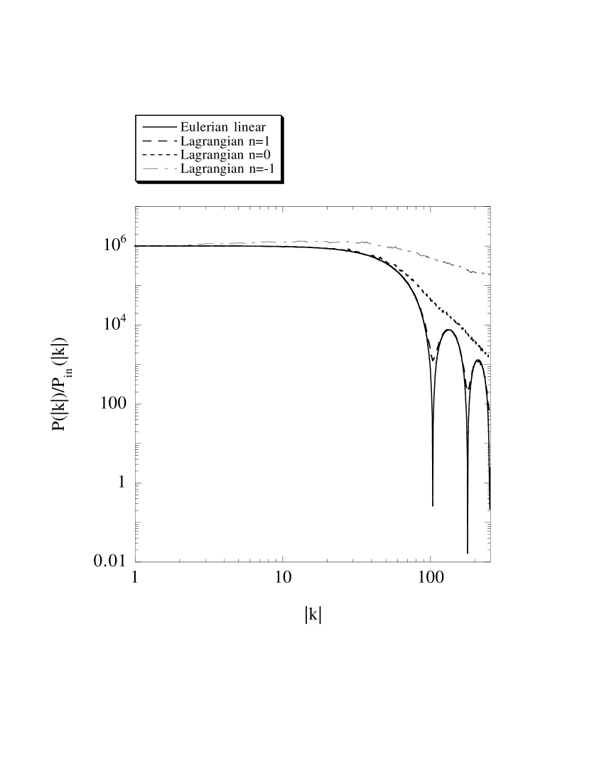
Figure 1: The ‘transfer function’ of density perturbations at $a=1000$ computed by the Eulerian linear theory, and Lagrangian first-order approximations. It does not depend on the initial conditions in the Eulerian linear theory, but does in the Lagrangian approximation.

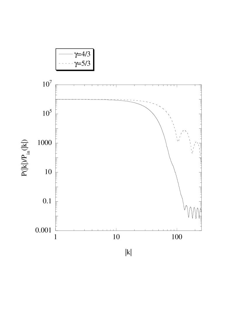
Figure 2: The ‘transfer function’ of density perturbations at $a=1000$ computed by the Lagrangian first-order approximation in the $\gamma=4/3$ and $5/3$ cases. Small-scale perturbations in the $\gamma=5/3$ case are developed more effectively than in the $\gamma=4/3$ case.

In our previous paper, we compared the Eulerian linear theory and the Lagrangian approximations in the $\gamma=4/3$ case, where the Jeans wavenumber $k_{\rm J}$ is a constant. In this case, the Eulerian linear density perturbations with wavenumbers smaller than a constant wavenumber always grow, while those with wavenumbers larger than that always decay with acoustic oscillation because of the constancy of the Jeans wavenumber. On the other hand, in the Lagrangian approximations, small-scale perturbations are developed by the nonlinear effect, and as a result, the difference between the Eulerian and the Lagrangian approximations becomes large especially at high-frequency region. (See Fig. 2 of Ref. moritate .)

Now we observe the results of the $\gamma=5/3$ case, Fig. 1. In this case, the Jeans wavenumber depends on time, and it becomes about $2500$ at $a=1000$ whereas it is set as $80$ at the initial time. This means that the Eulerian linear density perturbations with wavenumbers between $80$ and $2500$ are initially oscillating, but become growing modes later. Actually we can see this tendency at high-frequency region in Fig. 1. As for the Lagrangian approximation, small-scale perturbations are enhanced because of the nonlinear effect, as in the $\gamma=4/3$ case. The difference between the Eulerian and the Lagrangian approximations is, however, not so large because of the behavior of the Eulerian density perturbations mentioned above.

For comparison of the $\gamma=4/3$ and $5/3$ cases in the Lagrangian first-order approximation, we show in Fig. 2 the transfer function for both the cases, using the same initial conditions. This figure tells us that the growth of density perturbations computed by the Lagrangian approximation is suppressed by the pressure more weakly in the $\gamma=5/3$ case. This implies that the curious behavior of the Lagrangian perturbation solutions is preserved even if we observe it in the Eulerian coordinates.

V.2 Density field in a two-dimensional model

Next we consider an illustration in a two-dimensional model. In a dust model, Buchert and Ehlers bueh93 showed the density field with the Zel’dovich and the ‘post-Zel’dovich’ approximations. Following their illustrations, we present a realization of the density field (mapped by $128^{2}$ particles) with our approximations, in order to see how the pressure effect appears in a spatial pattern. We set the initial conditions for the scalar function $S(\bm{q},t)$ as

$$S(\bm{q},t_{\rm in})=\mu\sum_{K_{1}}\sum_{K_{2}}\frac{1}{K_{1}^{2}+K_{2}^{2}}\left[\cos(K_{1}q_{1}+K_{2}q_{2}+\phi(K_{1},K_{2}))\right]\,,$$ (74)

$$K_{1}^{2}+K_{2}^{2}\neq 0,\quad K_{1,2}=0,1,\cdots,5\,,$$

where the phases $\phi(K_{1},K_{2})$ are random numbers between $0$ and $2\pi$, and the amplitude $\mu$ is chosen so that $\mu=3.0\times 10^{-3}$. The periodic boundary condition is imposed. We consider the cases in which the equation of state is given as $P=\kappa\rho^{4/3}$ and $P=\kappa\rho^{5/3}$, assuming the Jeans wavenumber $K_{\rm J}\simeq 8$.

Figure 3: The particular density field of a two-dimensional model at $a=1000$. Shell crossings just occur in the dust case. (a) First-order approximation without pressure (the Zel’dovich approximation). (b) Second-order approximation without pressure (the ‘post-Zel’dovich’ approximation). (c) First-order approximation with pressure, $\gamma=4/3$. (d) Second-order approximation with pressure, $\gamma=4/3$. (e) First-order approximation with pressure, $\gamma=5/3$.

Figure 4: The particular density field of a two-dimensional model at $a=3000$. Shell crossings just occur in the $\gamma=4/3$ case. (a) First-order approximation without pressure (the Zel’dovich approximation). (b) Second-order approximation without pressure (the ‘post-Zel’dovich’ approximation). (c) First-order approximation with pressure, $\gamma=4/3$. (d) Second-order approximation with pressure, $\gamma=4/3$. (e) First-order approximation with pressure, $\gamma=5/3$.

Setting the initial conditions at $a=1$, the time evolution of the density field is shown in Figs. 3 and 4. In the $\gamma=4/3$ case, the evolution obviously proceeds slowly because of the pressure effect. In Fig. 3, shell crossings just arise in the dust case, while the evolution remains still quasi-nonlinear regime in the $\gamma=4/3$ case ($|\delta|\leq 1.0$). In Fig. 4, shell crossings are being formed in the $\gamma=4/3$ case, while in the dust case high-density structures are being dissolved. In these figures, the difference between the first- and second-order approximations seems still small on large scales (compare (a) and (b), and (c) and (d)), although the second-order solutions should compensate shortcomings of the first-order approximation on small scales, as was discussed by Buchert and Ehlers bueh93 for the dust case.

Above we have mentioned the $\gamma=4/3$ case, but what will happen if we take larger value of $\gamma$ such as $5/3$? To answer this question, we show in Figs. 3 (e) and 4 (e) the results computed by the Lagrangian first-order approximation in the $\gamma=5/3$ case. (The results by the Lagrangian second-order approximation are omitted, because we may presume them easily from other results presented.) As we stated in Secs. III and IV, the pressure effect in this case becomes weaker than in the $\gamma=4/3$ case. Indeed we see that the spatial density pattern resembles that in the dust case, rather than that in the $\gamma=4/3$ case.

In our perturbation scheme, shell crossings arise in the $\gamma=4/3$ and $5/3$ cases in spite of the presence of the pressure effect, but the features of first collapsing objects are manifestly different from those in the dust case. (Compare, e.g. Figs. 3 (a) and 4 (c).) The growth of small-scale structures is particularly suppressed because of the pressure effect, and therefore the size of overdense region becomes larger, as if the density field was spatially coarse-grained. (Compare, e.g. Figs. 4 (a) and (c).) Consequently our perturbation scheme may work like the ‘truncated Zel’dovich approximation’ cms ; mps ; ssmpm , which yields a coarse-grained density field of the original Zel’dovich approximation.

VI Discussion and Concluding Remarks

We have developed a perturbation theory in the Lagrangian hydrodynamics for a cosmological fluid with pressure. Hydrodynamic equations in the Lagrangian coordinates have been solved perturbatively up to second order, extending our earlier work. In our earlier work moritate , we solved the first-order perturbation equations in the Einstein-de Sitter background, and the second-order ones explicitly for the case $\gamma=4/3$. In this paper, we have obtained the first-order solutions in non-flat backgrounds and flat backgrounds with $\Lambda\neq 0$, and the approximate second-order solutions for the case $\gamma>4/3$. We have found that in several cases, the first-order solutions are written in terms of Gauss’ hypergeometric function. We have also presented illustrations in one- and two-dimensional systems, showing how our approximation theory describes the evolution of cosmological inhomogeneities.

In Sec. V, we have computed the power spectra of density perturbations in a one-dimensional model for the case $\gamma=5/3$ with the Eulerian linear theory and the Lagrangian first-order approximation, and have shown some amount of the difference between them. Our numerical calculations have also shown the difference between the Lagrangian first-order and second-order approximations, smaller than that in the $\gamma=4/3$ case. Let us investigate the reason of the smallness by considering single-wavemode perturbations and evaluating the ratio of the second- to the first-order solution, as we did in subsection 4.4 of Ref. moritate . We assume that the first-order solution is written as

$$S(q_{1},t)=\frac{\epsilon}{K^{2}}{\rm Re}\left[\left(c^{+}(K)D^{+}(K,t)+c^{-}(K)D^{-}(K,t)\right)\exp(iKq_{1})\right]\,,$$ (75)

where $\epsilon$ is the amplitude of the initial density perturbations, $c^{\pm}(K)$ denote constants of $O(1)$, and $D^{\pm}(K,t)$ are given by Eq. (44). Then, from Eq. (50), the second-order solution becomes

$$\zeta(q_{1},t)\sim-\frac{\epsilon^{2}}{4\pi}{\rm Re}\left[F_{1}(2K,K,t)\exp(i2Kq_{1})\right]\,.$$ (76)

For a concrete estimation, we assume $A|K|t^{-\gamma+4/3}\ll 1$ and use the approximation formulae, Eq. (56), for the cases $\gamma>4/3$. This assumption is reasonable because this is equivalent to taking into account perturbation modes whose Lagrangian wavenumbers are smaller than the Jeans wavenumber. The first-order and second-order solutions are then reduced to

$$S(q_{1},t) \sim \frac{\epsilon}{K^{2}}\left(\frac{A|K|}{2}\right)^{\nu}t^{2/3}\,{\rm Re}[\exp(iKq_{1})]\,,$$ (77)

$$\zeta(q_{1},t) \sim -\epsilon^{2}A^{2}\left(\frac{A|K|}{2}\right)^{2\nu}t^{-2\gamma+4}\,{\rm Re}[\exp(i2Kq_{1})]\,,$$ (78)

where $\nu=5/(8-6\gamma)$, and thus we find

$$\left|\frac{\zeta(q_{1},t)}{S(q_{1},t)}\right|\lesssim\epsilon\left(\frac{A|K|}{2}\right)^{\nu+2}t^{-2\gamma+10/3}\sim\epsilon\left(\frac{K}{K_{\rm J}}\right)^{2}\left(\frac{A|K|}{2}\right)^{\nu}t^{2/3}\,.$$ (79)

Note that the factor $\epsilon(A|K|/2)^{\nu}t^{2/3}$ corresponds to the Eulerian linear density perturbation and is of order unity at most in our case. Then we can show that $|\zeta/S|\ll 1$, since the assumption $A|K|t^{-\gamma+4/3}\ll 1$ is equivalent to $|K|/K_{\rm J}\ll 1$.

In the above estimation, the second-order solution $\zeta(q_{1},t)$ is of purely pressure origin because of the one-dimensionality, and thus can be regarded as a measure of the ‘second-order pressure effect’. Manifestly the effect of $\zeta(q_{1},t)$ becomes weaker in time as we take the larger value of $\gamma$. This curious fact is exactly the same as what we have addressed at the end of Secs. III and IV. Now let us examine the cause of the fact. We remark the terms of pressure origin in the perturbation equations, Eqs. (20), (IV), and (38). Then we see that all the terms of pressure origin have time-dependent coefficients such as ${\rm d}P/{\rm d}\rho(\rho_{\rm b})$ and ${\rm d}^{2}P/{\rm d}\rho^{2}(\rho_{\rm b})\rho_{\rm b}$, which behave as

$$\frac{{\rm d}P}{{\rm d}\rho}(\rho_{\rm b})\propto\frac{{\rm d}^{2}P}{{\rm d}\rho^{2}}(\rho_{\rm b})\rho_{\rm b}\propto a^{-3\gamma+3}\,,$$

under the assumption $P\propto\rho^{\gamma}$. These coefficients originate from the perturbation scheme, and we can safely claim that these coefficients yield the curious behavior of the perturbation solutions. In addition, these coefficients will appear at any order in the perturbation scheme, and therefore the curious behavior will arise, i.e. the larger value of $\gamma$ will produce the weaker effect of pressure at any order, as far as we consider the Lagrangian perturbation scheme. Our two-dimensional illustration also indicates how the evolution of inhomogeneities is sensitive to the variation of $\gamma$; the pressure works effectively in the $\gamma=4/3$ case, but does not in the $\gamma=5/3$ case, although it depends on the choice of values of parameters in general. Buchert et al. bdp argued that the $\gamma=2$ case corresponds to the adhesion approximation gurbatov , but, considering our illustration, it seems difficult to realize the adhesion-like approximation in the $\gamma=2$ case within the Lagrangian perturbation scheme.

However, there should be no such curious matter in the exact level of hydrodynamic equations. To see this, let us consider the one-dimensional case, where the relation between the Eulerian and the Lagrangian coordinates are given as

$$x_{1}=q_{1}+s_{1}(q_{1},t)\,,\quad x_{2}=q_{2}\,,\quad x_{3}=q_{3}\,.$$ (80)

Under the assumption $P=\kappa\rho^{\gamma}$, the exact equation for $s_{1}$ is adler ; moritate

$$\ddot{s_{1}}+2\frac{\dot{a}}{a}\dot{s_{1}}-4\pi G\rho_{\rm b}s_{1}-\frac{\kappa\gamma\rho_{\rm b}^{\gamma-1}}{a^{2}}\frac{s_{1,11}}{(1+s_{1,1})^{1+\gamma}}=0\,,$$ (81)

where the fourth term of the left-hand side holds the pressure effect. This term also has the time-dependent coefficient, ${\rm d}P/{\rm d}\rho(\rho_{\rm b})$, but simultaneously includes the effect of inhomogeneities by $(1+s_{1,1})^{1+\gamma}$ in the denominator. As long as $|s_{1,1}|\ll 1$, the results of the perturbation theory are reproduced, but once the flow lines of the fluid approach to the shell-crossing singularities, $1+s_{1,1}\rightarrow 0$, the effect of inhomogeneities becomes strong. In this situation, the larger value of $\gamma$ gives the stronger effect of pressure, and thus no curious matter will arise.

In our earlier work, and also in this work, we have experienced the shell-crossing problem in spite of taking into account the pressure effect. However, we can expect that this problem will also be avoided in the exact level, because the fourth term of the left-hand side of Eq. (81) will become very large near shell crossing, $1+s_{1,1}\rightarrow 0$, and will stop the growth of density enhancement. (Some implication may be obtained by Götz goetz , who solved the one-dimensional exact equation for the case $\gamma=1$ without cosmic expansion.)

The above discussion implies that we have to admit that our perturbation scheme yields some artificial results. This is true, but the Lagrangian perturbation scheme is a natural way to solve the hydrodynamic equations in cosmology, and our formulation will give a useful tool for large-scale structure formation in a practical sense. It is, in principle, applicable to any cosmological situation in which velocity dispersion arises and is written as a function of the density only. Actually Fig. 4 has shown that our scheme works better than the Zel’dovich approximation beyond shell crossing, giving some kind of spatial coarse graining of the density field, as is given by the truncated Zel’dovich approximation cms ; mps ; ssmpm . Detailed analyses of comparison of our scheme and the truncated Zel’dovich approximation (and also the adhesion approximation) will be provided in a separate publication.

As for the shell-crossing problem, Matarrese and Mohayaee mamo have treated it in Lagrangian perturbative approach for two-component fluid. They also experienced shell crossing in usual perturbative Lagrangian approach, and introduced the ‘stochastic adhesion’ model to overcome the problem. It will be interesting to probe how to treat the dynamics when shell crossing is occurring, or how to avoid shell crossing by taking account of the pressure effect in a sophisticated manner.

- (1) S. Weinberg, Gravitation and Cosmology (John Wiley & Sons, New York, 1972).
- (2) P. J. E. Peebles, The Large-Scale Structure of the Universe (Princeton University Press, Princeton, NJ, 1980).
- (3) T. Padmanabhan, Structure formation in the universe (Cambridge University Press, Cambridge, 1993).
- (4) P. Coles and F. Lucchin, Cosmology: The Origin and Evolution of Cosmic Structure (John Wiley & Sons, Chichester, 1995).
- (5) V. Sahni and P. Coles, Phys. Rep. 262, 1 (1995).
- (6) Ya. B. Zel’dovich, Astron. Astrophys. 5, 84 (1970).
- (7) T. Buchert, Mon. Not. R. Astron. Soc. 254, 729 (1992).
- (8) D. Munshi, V. Sahni, and A. A. Starobinsky, Astrophys. J. 436, 517 (1994).
- (9) M. Davis, G. Efstathiou, C. S. Frenk, and S. D. M. White, Astrophys. J. 292, 371 (1985).
- (10) S. N. Gurbatov, A. I. Saichev, and S. F. Shandarin, Mon. Not. R. Astron. Soc. 236, 385 (1989).
- (11) T. Buchert and A. Domínguez, Astron. Astrophys. 335, 395 (1998).
- (12) J. Binney and S. Tremaine, Galactic Dynamics (Princeton University Press, Princeton, NJ, 1987).
- (13) T. Buchert, A. Domínguez, and J. Perez-Mercader, Astron. Astrophys. 349, 343 (1999).
- (14) A. Domínguez, Phys. Rev. D 62, 103501 (2000).
- (15) A. Domínguez, astro-ph/0106288.
- (16) A. Domínguez, astro-ph/0103313.
- (17) S. Adler and T. Buchert, Astron. Astrophys. 343, 317 (1999).
- (18) M. Morita and T. Tatekawa, Mon. Not. R. Astron. Soc. 328, 815 (2001).
- (19) T. Buchert and J. Ehlers, Mon. Not. R. Astron. Soc. 264, 375 (1993).
- (20) P. Coles, A. L. Melott, and S. F. Shandarin, Mon. Not. R. Astron. Soc. 260, 765 (1993).
- (21) A. L. Melott, T. F. Pellman, and S. F. Shandarin, Mon. Not. R. Astron. Soc. 269, 626 (1994).
- (22) B. S. Sathyaprakash, V. Sahni, D. Munshi, D. Pogosyan, and A. L. Melott, Mon. Not. R. Astron. Soc. 275, 463 (1995).
- (23) G. Götz, Class. Quantum Grav. 5, 743 (1988).
- (24) S. Matarrese and R. Mohayaee, Mon. Not. R. Astron. Soc. 329, 37 (2002).