Recent Developments in Magnetic Dynamo Theory

Abstract

Two spectral regimes of magnetic field amplification in magnetohydrodynamic (MHD) flows can be distinguished by the scale on which fields are amplified relative to the primary forcing scale of the turbulence. For field amplification at or below the forcing scale, the amplification can be called a “small scale dynamo.” For amplification at and above the forcing scale the process can be called a “large scale dynamo.” $Non-local$ (in wave number) effects play a key role in both the growth of the small scale field in non-helical turbulence and the growth of large and small scale fields in helical turbulence. Mean field dynamo (MFD) theory represents a simple semi-analytic way to get a handle on large scale field amplification in MHD turbulence. Helicity has long been known to be important for large scale, flux generating, externally forced MFDs. The extent to which such MFDs operate “slow” or “fast” (dependent or independent on magnetic Reynolds number) has been controversial, but there has been recent progress. Simulations of $\alpha^{2}$ dynamos in a periodic box dynamo and their quenching can now be largely understood within a simplified dynamical non-linear paradigm in which the MFD growth equation is supplemented by the total magnetic helicity evolution equation. For $\alpha^{2}$ dynamos, the large scale field growth is directly related to the large scale magnetic helicity growth. Magnetic helicity conservation then implies that growth of the large scale magnetic helicity induces growth of small scale magnetic (and current) helicity of the opposite sign, which eventually suppresses the $\alpha$ effect driving the MFD growth. Although the $\alpha^{2}$ MFD then becomes slow in the long time limit, substantial large scale field growth proceeds in a kinematic, “fast” phase before non-linear asymptotic quenching of the “slow” phase applies. Ultimately, the MFD emerges as a process that transfers magnetic helicity between small and large scales. How these concepts apply to more general dynamos with shear, and open boundary dynamos is a topic of ongoing research. Some unresolved issues are identified. Overall, the following summarizes the most recent progress in mean-field dynamo theory:

For a closed turbulent flow,

the non-linear mean field dynamo,

is first fast and kinematic, then slow and dynamic,

and magnetic helicity transfer makes it so.

(to appear in “Turbulence and Magnetic Fields in Astrophysics,” eds. E. Falgarone and T. Passot, Springer Lecture Notes in Physics)

1 Small Scale vs. Large Scale Field Amplification

A dynamo is a process which exponentially amplifies or sustains magnetic energy in the presence of finite dissipation. In this paper I will focus on magnetohydrodynamic (MHD) dynamos, where the only flux dissipating term in Ohm’s law for the total magnetic field is the resistive term.

The simple definition of a dynamo given above does not distinguish the scale on which the magnetic energy is sustained against turbulent forcing, whether a net flux is produced in the spatial region of interest, or the nature of the forcing (e.g. shear driven or isotropically forced). It is helpful to distinguish between “small scale dynamos” which describe field generation at or below the turbulent forcing scale, and “large scale dynamos” which describe field generation on scales larger than the forcing scale. Both present their own set of problems.

For the Galaxy, supernovae dominate the nearly isotropic turbulent forcing, and although there is a range of forcing scales, typically the dominant scale is $\sim 50-100$pc ruz . A cascade leads to a nearly Kolmogorov turbulent kinetic energy spectrum. Faraday rotation and synchrotron polarization observations reveal the presence of a random component of the Galactic field, also with a dominant scale of $\sim 50-100$ parsecs, and an ordered toroidal field on the scale of $\mathrel{\hbox to0.0pt{\lower 4.0pt\hbox{\hskip 1.0pt$\sim$}\hss}\raise 1.0pt\hbox{$>$}}1$kpc

An important point about large scale field growth is that regardless of long standing debates about whether the large scale fields of the Galaxy is primordial or produced in situ, kulsrudetal ; zweibel ; ccm and regardless of similar debates about the origin of large scale, jet producing, poloidal fields in accretion disks (e.g. lpp ) one thing we do know is that the Sun, at least $must$ have a large scale dynamo operating because the mean flux reverses sign every 11 years. If the flux were simply flux frozen into the sun’s formation from the protostellar gas, we would not expect such reversals.

For both small and large scale dynamos, the richness and the complication of dynamo theory is the non-linearity of the MHD equations. To really understand the theory, we need to understand the backreaction of the growing magnetic field on the turbulence, the saturated spectra of the magnetic field, and the spectral evolution time scales. Do theoretical and numerical calculations make predictions which are consistent with what is observed in astrophysical systems or not? What are the limitations of these predictions?

1.1 Small Scale Dynamo

The “small scale dynamo” describes magnetic field amplification on and below the turbulent forcing scale (e.g. kazanstev ; parker ; zeldovich ). Field energy first builds up to equipartition with the kinetic energy on the smallest scales kulsrud because the growth time is the turnover time, the turnover times are shorter for smaller scales, and the equipartition level is lower for the small scales. The fast growth, seen in non-linear simulations, can be predicted analytically kazanstev ; parker ; zeldovich ; kulsrud . The approach to near equipartition is not controversial but the shape of the saturated small scale spectrum needs more discussion, particularly for the Galaxy.

Recent simulations of forced non-helical turbulence for magnetic Prandtl number ($Pr\equiv\nu_{v}/\nu_{M}$, where $\nu_{v}$ is the viscosity and $\nu_{M}$ is the magnetic diffusivity) satisfying $Pr\geq 1$ in a periodic box have shown that the field does not build up to anywhere near equipartition on the input scale of the turbulence kida91 ; maroncowley . Rather, the field piles up on the smallest scales. The interpretation is that the forcing scale velocity directly shears the field into folds or filaments with length of order the forcing scale but with cross field scale of order the resistive scale, accounting for the spectral power at small scales. (see scmm for a careful semi-analytic study of the $Pr>>1$ case). Since the small scale field is amplified by shear directly from the input scale, one can argue that there is a $non-local$ direct cascade.

How does the observed small scale field of the Galaxy compare with the above results? Since observations show near equipartition of the field energy with the kinetic energy at the forcing scale beck , there is a discrepancy between the observations and the numerical simulation results for non-helical turbulence.

A possible resolution might arise from the idealized problem, explored in maronblackman . When the turbulence is forced with sufficient kinetic helicity $\langle{\bf v}\cdot\nabla\times{\bf v}\rangle$, the spectrum changes in an important way. Figures 1 and 2 below come from 3-D MHD simulations in which kinetic energy is forced in a box, and the helical fraction of the kinetic forcing is varied ($f_{h}=1$ corresponds to maximal helical forcing). The forcing wave number is $k/2\pi=4.5$. For sufficiently large $f_{h}$, (determined by that for which the kinematic $\alpha^{2}$ dynamo can grow) the magnetic spectrum grows two peaks, one at $k/2\pi=1$ and one at the forcing scale. The kinetic helicity thus influences both the small and large scale field growth.

Whether these results apply to the Galaxy or protogalaxy is unclear since those systems have shear (see also vishniac ), boundaries, and stratification unlike the simulations of maronblackman . But the principle that the large $and$ small scale fields are both influenced by helicity has been demonstrated.

The emergence of two peaks motivates a two-scale approach which is a great simplification that will be exploited later. The shift of the small scale peak to the forcing scale is less understood than the generation of the large scale field. I now discuss the latter.

Figure 1: Saturated kinetic and magnetic energy spectra for successive values of fractional helicity $f_{h}$.

Figure 2: Time sequence of kinetic and magnetic energy spectra for $f_{h}=1$

1.2 Large Scale Dynamo

The large scale field of the Galaxy beck ; zweibel seems to be of quadrapole mode and therefore the planar component of the large scale field has the same sign across the mid-plane. The toroidal field reverses on scales of a few kpc in radius In these annuli, there appears to be a net toroidal flux when integrated over the full height of the Galaxy. If this inference continues to survive future observations, the mechanism for field production must produce a net toroidal flux in annuli that extend the full vertical disk thickness, not just a net magnetic energy.

A leading framework for understanding the in situ origin of large scale magnetic field energy and flux growth in galaxies and stars, and even for the peak in the large scale magnetic energy in the helically forced case of Figure 1 (see also b2001 ) has been the mean field dynamo (MFD) theory ruz ; parker ; zeldovich ; moffatt ; krause . The theory appeals to some combination of helical turbulence (leading to the $\alpha$ effect), differential rotation (the $\Omega$ effect), and turbulent diffusion (the $\beta$ effect) to exponentiate an initial seed mean magnetic field. Ref. steenbeck developed a formalism for describing the concept parker that helical turbulence can twist toroidal ($\phi$) fields into the poloidal ($r,z$) direction, where they can be acted upon by differential rotation to regenerate a powerful large scale toroidal magnetic field. The turbulent diffusion serves to redistribute the flux so that inside the bounded volume of interest, a net flux can grow.

The formalism separates the total magnetic field into a mean component $\overline{\bf B}$ and a fluctuating component ${\bf b}$, and similarly for the velocity field ${\bf V}$. The mean can be a spatial or ensemble average. The ensemble average is approximately equal to the spatial average when there is a scale separation between the mean and fluctuating scales. In reality, the scale separation is often weaker than the dynamo theorist desires, though a weak separation is also helpful given the limited dynamic range of simulations. I proceed to consider spatial averages to simplify the discussion. (Please also note that non-helical large scale field generation exists from the magnetorotational instability (MRI) balbus but I do not consider this here and focus on externally forced systems. Actually the helical MFD dynamo may be operating even in systems with the MRI. Also I do not consider the model of vishniac here as that will be covered elsewhere in this volume.)

The mean field $\overline{\bf B}$ satisfies the induction equation moffatt ; steenbeck

$${\partial\overline{\bf B}\over\partial t}=-c\nabla\times\overline{\bf E},$$ (1)

where

$$\overline{\bf E}=-\left(\overline{\bf V}\times\overline{\bf B}\right)/c-\langle{\bf v}\times{\bf b}\rangle/c+\nu_{M}\nabla\times\overline{\bf B},$$ (2)

$$\langle{\bf v}\times{\bf b}\rangle_{i}=\alpha_{ij}{\overline{B}}_{j}-\beta_{ijk}\partial_{j}{\overline{B}}_{k}$$ (3)

is the turbulent electromotive force (EMF), and $\nu_{M}=\eta c^{2}/4\pi$ is the magnetic diffusivity defined with the resistivity $\eta$. Here $\alpha_{ij}$ contains Parker’s twisting (the $\alpha$ effect) and $\beta_{ijk}$ contains the turbulent diffusivity. Ref. steenbeck calculated $\overline{\bf E}$ to first order in $\overline{B}$ for isotropic $\alpha_{ij}$ and $\beta_{ijk}$ and hence the pseudo-scalar and scalar dynamo coefficients $\alpha$ and $\beta$ respectively to zeroth order in $\overline{B}$ from the statistics of the turbulence, ignoring the Navier-Stokes equation. When the Navier-Stokes equation is not used, we speak of the “kinematic theory.” Using the equation for the fluctuating field $\partial_{t}{\bf b}$, plugging it into $\langle{\bf v}\times{\bf b}\rangle$, the standard approach gives a kinematic $\alpha\propto-\int\langle{\bf v}(t)\cdot\nabla\times{\bf v}(t^{\prime})\rangle dt^{\prime}\sim-\tau_{c}\langle{\bf v}\cdot\nabla\times{\bf v}\rangle dt$ and $\beta\propto\int\langle{\bf v}(t)\cdot{\bf v}(t^{\prime})\rangle dt^{\prime}\sim\tau_{c}\langle{\bf v}\cdot{\bf v}\rangle dt$. I will come back to correcting the form for $\alpha$ in section 2.3 and 2.4. because we really want a fully dynamic theory, that accounts for the dynamo coefficients’ dependence on ${\bf b}$ and $\overline{\bf B}$. Only then can one fully address the fundamental problem of mean field dynamo theory: how does the growing magnetic field affect the rate and saturation level of growth?

Substituting (2) into (1), gives the MFD equation

$${\partial\overline{\bf B}\over\partial t}=\nabla\times\left(\overline{\bf V}\times\overline{\bf B}\right)+\nabla\times(\alpha\overline{\bf B})-\nabla\times(\beta+\lambda)\nabla\times\overline{\bf B}.$$ (4)

The first term on the right is the non-controversial $``\Omega-{\rm effect}.^{\prime\prime}$ If one assumes $\overline{\bf V}$, $\alpha$ and $\beta$ to be independent of $\overline{B}$, then (4) can be solved as a linear eigenvalue problem for the growing modes of $\overline{\bf B}$ in the Sun and other bodies. However a rapid growth of the fluctuating field necessarily accompanies the MFD in a turbulent medium. Its impact upon the growth of the mean field, and the impact of the mean field itself on its own growth have been controversial.

The controversy arises because Lorentz forces from the growing magnetic field react back on the turbulent motions driving the field growth kulsrud ; cowling ; piddington ; vc ; kitchatinov ; ch ; vainshtein . It is useful to distinguish between fast MFD action (also called “rapid” MFD action) and, slow MFD action (also called “resistively limited” MFD action). Fast MFD action proceeds at growth rates which do not go to zero as the magnetic Reynolds number $R_{M}\rightarrow\infty$, and maintain this property even when the non-linear backreaction from the magnetic field is included. Slow MFD action proceeds at rates that vanish as $R_{M}\rightarrow\infty$. I sometimes use “resistively limited” rather than “slow” because the former more explicitly describes the reduced action.

For galaxies and stars, conventional wisdom (which could be challenged brannach and see section 2.3) presumes that rapid MFD action is necessary if the observed large scale fields are to be wholly produced and sustained by the MFD, given observed cycle periods and available time scales. That this may not be the case is a separate issue from understanding what the theory can actually provide. The latter is the focus herein. If dynamos in stars and galaxies do operate fast, then we would like to understand how, in light of recent numerical and theoretical evidence for slow $\alpha^{2}$ dynamos in periodic boxes b2001 ; fb . What are the differences between these dynamos and real systems? where does the theory fail and where does the theory succeed?

There are several issues which must be disentangled. First is the role of magnetic helicity conservation in constraining dynamo theory. In the steady state, such constraints are strongly influenced by boundary conditions, so one must be careful to understand the differences when applying idealized equations for closed systems to real systems with boundaries. Time-dependent dynamical constraints require helicity conservation to be supplemented in some way by the Navier-Stokes equation. Then the fully dynamical evolution of $\alpha$ and the non-linear backreaction can be studied.

Two directions emerge. One is to produce a time dependent dynamical non-linear theory that fully agrees with numerical simulations in periodic boxes. This has recently been done fb . The second is to recognize that in real systems, there is physics which has not yet been comprehensively studied. This includes shear vishniac ; branshear , boundary terms which alleviate magnetic helicity conservation constraints, gravity, and a vertical variation of the dynamo coefficients. It has proven difficult in the simplest generalizations, to make the dynamo asymptotically fast brannach ; branshear , but this may not be needed in some applications (e.g. Galaxy) if a kinematic phase lasts long enough. This will be discussed in detail.

In section 2 I discuss the role of magnetic helicity conservation in dynamo theory. I first show that the escape of magnetic helicity through the boundaries might play an important role in maintaining fast MFD action during the steady sustenance phase of dynamos, and thus in interpreting quenching studies for this regime. I discuss the direct observational implications of the boundary terms and the fact that stars and disks harbor active coronae. I then show that the time dependent mean field dynamo is really a process by which magnetic helicity gets transferred from small to large scales by a non-local inverse cascade and that the time-dependent dynamical quenching in recent periodic box simulations can be understood in this framework fb . At late times, these box dynamos are resistively limited, depending sensitively on the magnetic Reynolds number, however the kinematic phase lasts quite awhile and this fact has very important implications. In the last part of section 2, I discuss an unsolved puzzle that arises in the derivation of the successful dynamical quenching model. In section 3, I summarize some key conclusions and pose open questions.

2 Magnetic Helicity Conservation and Dynamo Quenching

Although the MFD theory predates detailed studies of magnetohydrodynamic (MHD) turbulence, the MFD may be viewed as a framework for studying the inverse cascade of magnetic helicity. Whether this inverse cascade is primarily local (proceeding by interactions of eddies/waves of nearby wave numbers) or non-local (proceeding with a direct conversion of power from large to small wave numbers) is important to understand. The simple MFD seems to be consistent with the latter b2001 .

From the numerical solution of approximate equations describing the spectra of energy and helicity in MHD turbulence, Ref. pfl showed that the $\alpha$ effect conserves magnetic helicity, $H_{M}=\int({\bf A}\cdot{\bf B})d^{3}x$, by pumping a positive (negative) amount to scales $>l$ (the outer scale of the turbulence) while pumping a negative (positive) amount to scales $\ll l$. Magnetic energy at the large scale was identified with the $\overline{\bf B}$ of Ref. steenbeck . Thus, dynamo action leading to an ever larger $\overline{B}$, hence the creation of ever more large scale helicity, can proceed as long as helicity of the opposite sign can be removed or dissipated. More on this in section 2.3. Here I first derive the general magnetic helicity conservation equations used to constrain the turbulent EMF, and investigate the implications of two steady state cases in detail before considering the time dependent case and interpretation of dynamo simulations.

Using Ohm’s law for the electric field,

$${\bf E}={-c^{-1}{\bf V}\times{\bf B}+\eta{\bf J}}$$ (5)

and averaging its dot product with ${\bf B}$, gives

$$\langle{{\bf E}\cdot{\bf B}}\rangle=\overline{\bf E}\cdot\overline{\bf B}+\langle{{\bf e}\cdot{\bf b}}\rangle=-c^{-1}\langle{{\bf v}\times{\bf b}}\rangle\cdot\overline{\bf B}+\eta\overline{\bf J}\cdot\overline{\bf B}+\langle{{\bf e}\cdot{\bf b}}\rangle$$ (6)

where ${{\bf J}}$ is the current density. A second expression for $\langle{\bf E}\cdot{\bf B}\rangle$ also follows from Ohm’s law without first splitting into mean and fluctuating components, that is

$$\langle{{\bf E}\cdot{\bf B}}\rangle=\eta\left\langle\bf J\cdot{\bf B}\right\rangle=\eta\overline{\bf J}\cdot\overline{\bf B}+\eta\langle{{\bf j}\cdot{\bf b}}\rangle=\eta\overline{\bf J}\cdot\overline{\bf B}+c^{-1}\nu_{M}\left\langle{\bf b}\cdot\nabla\times{\bf b}\right\rangle.$$ (7)

Using (7) and (6), we have

$$-c^{-1}\langle{{\bf v}\times{\bf b}}\rangle\cdot\overline{\bf B}=c^{-1}\lambda\left\langle{\bf b}\cdot\nabla\times{\bf b}\right\rangle-\langle{\bf e}\cdot{\bf b}\rangle,$$ (8)

which can be used to constrain $\langle{\bf v}\times{\bf b}\rangle$ in the mean field theory.

Now consider ${\bf E}$ in terms of the vector and scalar potentials ${\bf A}$ and $\Phi$:

$${\bf E}=-\nabla\Phi-(1/c)\partial_{t}{\bf A}.$$ (9)

Dotting with ${\bf B}=\nabla\times{\bf A}$ we have

$${\bf E}\cdot{\bf B}=-\nabla\Phi\cdot{\bf B}-(1/c){\bf B}\cdot\partial_{t}{\bf A}.$$ (10)

After straightforward algebraic manipulation and application of Maxwell’s equations, this equation implies

$${\bf E}\cdot{\bf B}=-(1/2)\nabla\cdot\Phi{\bf B}+(1/2)\nabla\cdot({\bf A}\times{\bf E})$$ (11)

$$-(1/2c)\partial_{t}({\bf A}\cdot{\bf B})=(-1/2c)\partial_{\mu}{H}^{\mu}({\bf B})=\eta\bf J\cdot{\bf B},$$ (12)

where

$$H^{\mu}({\bf B})=(H_{0},H_{i})=[{\bf A}\cdot{\bf B},c\Phi{\bf B}-c{\bf A}\times{\bf E}]$$ (13)

is the magnetic helicity density 4-vector fieldaip , and the contraction has been done with the 4 x 4 matrix $\eta_{\mu\nu}$ where $\eta_{\mu\nu}=0$ for $\mu\neq\nu$, $\eta_{\mu\nu}=1$ for $\mu=\nu=0$ and $\eta_{\mu\nu}=-1$ for $\mu=\nu>0$. Taking the average of (12) gives

$$\partial_{\mu}{\overline{H}}^{\mu}({{\bf B}})=-2c\langle{\bf E}\cdot{\bf B}\rangle=-2c\overline{\bf E}\cdot\overline{\bf B}-2c\langle{\bf e}\cdot{\bf b}\rangle=-2c\eta\langle\bf J\cdot{\bf B}\rangle.$$ (14)

If, instead of starting with the total ${\bf E}$ as in (9), I start with ${\bf e}$ and then dot with ${\bf b}$ and average, the analagous derivation replaces (14) by

$$\partial_{\mu}{\overline{H}}^{\mu}({\bf b})=-2c\langle{{\bf e}}\cdot{{\bf b}}\rangle,$$ (15)

where ${\overline{H}}^{\mu}({\bf b})$ indicates the average of ${H}^{\mu}({\bf b})$. The latter is defined like (13) but with the corresponding fluctuating quantities replacing the total quantities. Similarly, starting with $\overline{\bf E}$ and dotting with $\overline{\bf B}$, gives

$$\partial_{\mu}H^{\mu}(\overline{\bf B})=-2c{\overline{\bf E}}\cdot{\overline{\bf B}},$$ (16)

where ${H}^{\mu}(\overline{\bf B})$ is defined as in (13) but with the corresponding mean quantities replacing the total quantities.

In the next three subsections, I consider the implications of magnetic helicity conservation for 3 separate cases. In the first I assume a steady state and ignore boundary terms. In the second, I include boundary terms but still demand a steady state. The third is the case in which boundaries are ignored, but a full time evolution of $\alpha$ is considered and a fully dynamical theory is obtained that agrees with recent numerical simulations.

2.1 Case 1: Homogeneous, Stationary Turbulence in Periodic Box

Consider statistically stationary turbulence, where the averaging is over periodic boundaries. Then, the spatial divergence terms on the left of (14) become surface integrals and vanish. Discarding the spatial divergenece terms in (15) gives

$$\langle{{\bf e}}\cdot{{\bf b}}\rangle=-{1\over 2c}\partial_{t}\langle{\bf a}\cdot{{\bf b}}\rangle.$$ (17)

In the steady state, (17) vanishes and eqn (8) shows that $\langle{\bf v}\times{\bf b}\rangle$ is resistively limited.

If a uniform $\overline{\bf B}$ is imposed over the periodic box, then $\overline{\bf B}$ cannot change with time, and has no gradients. This is the case of Ref. ch , which measures $\alpha$ but cannot test for MFD action. No mean quantity varies on long time scales. In this case, (8) then implies

$$-c^{-1}\langle{{\bf v}\times{\bf b}}\rangle\cdot\overline{\bf B}=\alpha{\overline{\bf B}}^{2}/c=c^{-1}\lambda\left\langle{\bf b}\cdot\nabla\times{\bf b}\right\rangle,$$ (18)

where $\alpha=\alpha_{33}$ for a uniform field in the $z$ direction. Rearranging gives

$$|\alpha|=\left|{\lambda\left\langle{\bf b}\cdot\nabla\times{\bf b}\right\rangle\over\overline{\bf B}^{2}}\right|.$$ (19)

We then have

$$|\alpha|\mathrel{\hbox to0.0pt{\lower 4.0pt\hbox{\hskip 1.0pt$\sim$}\hss}\raise 1.0pt\hbox{$<$}}\left|{{k_{2}b_{2}^{2}}\tau_{2}\over R_{M,2}^{n}\overline{\bf B}^{2}/v_{2}^{2}}\right|\sim\left|{\alpha_{0}\over R_{M,2}^{n}\overline{\bf B}^{2}/b_{2}^{2}}\right|$$ (20)

where $b_{2}$ and $v_{2}$ are the fluctuating field magnetic energy of the dominant energy containing eddies (which is the forcing scale for both $v$ and $b$ for $f_{h}=1$ turbulence as described in section 1), $k_{2}$ is the wavenumber for that scale (= the forcing scale), and $n=3/4$ if the current helicity is dominated by large wavenumber and $n=1$ if it is dominated by small wavenumbers. The quantity $\tau_{2}$ is the associated eddy turnover time and $R_{M,2}=v_{2}/k_{2}\nu_{M}$ is the magnetic Reynolds number associated with the forcing scale. Assuming a steady state, I used $v_{2}\sim b_{2}$ which is roughly consistent with numerical results. Then assuming forcing with maximal kinetic helicty, I replaced the numerator with $\alpha_{0}$, the maximum possible value of a helical quantity of that dimension.

Pouquet Correction and Connection to Previous Studies:

If we now take $\alpha$ to be of the form first derived by pfl , (discussed further in section 2.3) in the context of a maximally helical, force free $\alpha^{2}$ dynamo in a periodic box, we have

$$\alpha=-(1/3)\tau(\langle{\bf v}\cdot\nabla\times{\bf v}\rangle-\langle{\bf b}\cdot\nabla\times{\bf b}\rangle),$$ (21)

where $\tau$ is the correlation time of the turbulence at $k_{2}$. Consider the implications of this formula in the steady state. If we use (17) in (8), and allow for a non-uniform mean field it is straightforward to show that $\alpha$ can be written

$$\alpha={\alpha_{0}+R_{M,2}\beta\langle{\overline{\bf B}\cdot\nabla\times\overline{\bf B}}\rangle/{B^{2}_{eq}}\over 1+R_{M,2}\overline{B}^{2}/B_{eq}^{2}}.$$ (22)

Note that brackets around the current helicity are present because we allow for the fact that the mean field can have a scale smaller than the overall system (or box) scale. For example, the growth of the mean field at wavenumber $k=1$ in a periodic box can occur when the $k=0$ field is zero. Indeed, the limit of this equation for a mean field of zero curl produces exactly the result obtained numerically by ch result for uniform $\overline{\bf B}$. However, as is clear from this formula, it only emerges when $\overline{\bf B}$ is uniform and the system is in a steady state.

For steady-state but non-uniform $\overline{\bf B}$ in the simplest case of a maximally helical $\alpha^{2}$ dynamo in periodic box with no shear, the field energy and large scale helicity sustenance depend on $\overline{\bf E}\cdot\overline{\bf B}$. If we assume for example that $\beta=\beta_{0}=$constant (unquenched, one extreme limit) and ignore mean velocities, and use (22)

$$\begin{array}[]{r}-\langle\overline{\bf E}\cdot\overline{\bf B}\rangle=\alpha\langle\overline{B}^{2}\rangle-\beta\langle\overline{\bf B}\cdot\nabla\times\overline{\bf B}\rangle={\alpha_{0}+R_{M,2}\beta_{0}\langle{\overline{\bf B}\cdot\nabla\times\overline{\bf B}}\rangle/B_{eq}^{2}\over 1+R_{M,2}\overline{B}^{2}/B_{eq}^{2}}\langle\overline{B}^{2}\rangle-\beta_{0}\langle\overline{\bf B}\cdot\nabla\times\overline{\bf B}\rangle\\ ={\alpha_{0}\over 1+R_{M,2}\langle\overline{B}^{2}\rangle/B_{eq}^{2}}\langle\overline{B}^{2}\rangle-{\beta_{0}\over 1+R_{M,2}\langle\overline{B}^{2}\rangle/B_{eq}^{2}}\langle\overline{\bf B}\cdot\nabla\times\overline{\bf B}\rangle,\end{array}$$ (23)

where $B_{eq}=v_{2}$ in velocity units. Notice that choosing a constant $\beta=\beta_{0}$ in the steady state, leads to an EMF that is resistively quenched, and is the same as that with an artificially imposed symmetric, resisitive quenching of $\alpha$ and $\beta$. These forms of $\alpha$ and $\beta$ are however misleading in the sense that although their combination is consistent with helicity conservation in the EMF, the division of $\alpha$ and $\beta$ in this way is not the division which was conistent with our initial assumption of $\beta=\beta_{0}$ and so their forms are mere artifacts bb . Actually, in the saturated state, the current helicities of the large and small scale must be equal and opposite b2001 ; fb ; bb (this follows from (14) with no divergence terms). We then have $\langle\overline{\bf J}\cdot\overline{\bf B}\rangle\propto\alpha-\alpha_{0}$. This implies, for our assumed $\beta=\beta_{0}$, and for large $R_{M,2}$ that

$$\alpha={\alpha_{0}\over 1+\langle\overline{B}^{2}\rangle/B_{eq}^{2}}.$$ (24)

This is the actual steady state form of $\alpha$ when $\beta$ is unquenched. Note that there is no $R_{M,2}$ depednence in the separate forms of $\alpha$ or $\beta$ even though $\overline{\bf E}\cdot\overline{\bf B}$ is resitively limited: in the steady state $\langle\overline{\bf E}\cdot\overline{\bf B}\rangle$ must satisfy $\langle\overline{\bf E}\cdot\overline{\bf B}\rangle=\nu_{M}\overline{\bf J}\cdot bbB\rangle$. Ultimately, one can solve for $\overline{B}$ to see this demonstrated.

If we were to instead assume $\alpha\propto\beta$ from the outset, one finds

$$\alpha={\alpha_{0}\over 1+R_{M,2}(\alpha/\alpha_{0}+\langle\overline{B}^{2}\rangle/B_{eq}^{2}-1)}.$$ (25)

Later we will see a deeper implication of the appearance of the current helicity in (18).

2.2 Case 2: Inhomogeneous Turbulence, Finite Boundary Terms and Implications for Coronal Activity in Steady State

Now consider a system (e.g. Galaxy or Sun) to have volume $<<$ universal volume. Integrating (12) over all of space, $U$, then gives

$$\int_{U}{\bf E}\cdot{\bf B}\ d^{3}x=-(1/2)\int_{U}\nabla\cdot\Phi{\bf B}\ d^{3}x+(1/2)\int_{U}\nabla\cdot({\bf A}\times{\bf E})\ d^{3}x$$ (26)

$$-(1/2c)\partial_{t}\int_{U}{\bf A}\cdot{\bf B}\ d^{3}x=-(1/2c)\partial_{t}{\mathcal{H}}({\bf B})=\int_{U}\eta{\bf J}\cdot{\bf B}d^{3}x,$$ (27)

where the divergence integrals vanish when converted to surface terms at infinity. I have defined the global magnetic helicity

$${\mathcal{H}}({\bf B})\equiv\int_{U}{\bf A}\cdot{\bf B}\ d^{3}x,$$ (28)

where $U$ allows for scales much larger than the mean field scales. It is easy to show that a parallel argument for the mean and fluctuating fields leads to

$$\partial_{t}{\mathcal{H}}(\overline{\bf B})=\partial_{t}\int_{U}\overline{\bf A}\cdot\overline{\bf B}\ d^{3}x=-2c\int_{U}\overline{\bf E}\cdot\overline{\bf B}\ d^{3}x$$ (29)

and

$$\partial_{t}{\overline{\mathcal{H}}}({\bf b})=\partial_{t}\int_{U}\langle{\bf a}\cdot{\bf b}\rangle\ d^{3}x=-2c\int_{U}\langle{\bf e}\cdot{\bf b}\rangle\ d^{3}x=-2c\int_{U}{\bf e}\cdot{\bf b}\ d^{3}x=\partial_{t}{{\mathcal{H}}}({\bf b}),$$ (30)

where the penultimate equality in (30) follows from redundancy of averages.

I now split (29) and (30) into contributions from inside and outside the rotator. One must exercise caution in doing so because ${\mathcal{H}}$ is gauge invariant and physically meaningful only if the volume $U$ over which ${\mathcal{H}}$ is integrated is bounded by a magnetic surface (i.e. normal component of ${\bf B}$ vanishes at the surface), whereas the surface separating the outside from the inside of the rotator is not magnetic in general. Ref. berger shows how to construct a revised gauge invariant quantity called the relative magnetic helicity,

$${\mathcal{H}}_{R,i}({\bf B}_{i})={\mathcal{H}}({{\bf B}}_{i},{\bf P}_{o})-{\mathcal{H}}({\bf P}_{i},{\bf P}_{o})$$ (31)

where the two arguments represent inside and outside the body respectively, and $\bf P$ indicates a potential field. The relative helicity of the inside region is thus the difference between the actual helicity and the helicity associated with a potential field inside that boundary. The use of ${\bf P}_{i}$ is not arbitrary in (31), and is in fact the field configuration of lowest energy. While (31) is insensitive to the choice of external field berger , it is most convenient to take it to be a potential field as is done in (31) symbolized by ${\bf P}_{o}$. The relative helicity of the outer region, ${\mathcal{H}}_{R,o}$, is of the form (31) but with the $o$’s and $i$’s reversed. The ${\mathcal{H}}_{R}$ is invariant even if the boundary is not a magnetic surface.

The total global helicity, in a magnetically bounded volume divided into the sum of internal and external regions, $U=U_{i}+U_{e}$, satisfies berger

$${\mathcal{H}}({\bf B})={\mathcal{H}}_{R,o}({\bf B})+{\mathcal{H}}_{R,i}({\bf B}),$$ (32)

when the boundary surfaces are planar or spherical. This latter statement results from the vanishing of an additional term associated with potential fields that would otherwise appear in (32). Similar equations apply for $\overline{\bf B}$ and ${\bf b}$, so (29) and (30) can be written

$$\partial_{t}{{\mathcal{H}}}(\overline{\bf B})=\partial_{t}{{\mathcal{H}}}_{R,o}(\overline{\bf B})+\partial_{t}{{\mathcal{H}}}_{R,i}(\overline{\bf B}),$$ (33)

and

$$\partial_{t}{{\mathcal{H}}}({\bf b})=\partial_{t}{{\mathcal{H}}}_{R,o}({\bf b})+\partial_{t}{{\mathcal{H}}}_{R,i}({\bf b})$$ (34)

respectively. According to equation (62) of Ref. 25,

$$\partial_{t}{{\mathcal{H}}}_{R,i}({\bf B})=-2c\int_{U_{i}}{{\bf E}\cdot{\bf B}}d^{3}x+2c\int_{DU_{i}}({\bf A}_{p}\times{{\bf E}})\cdot d{\bf S},$$ (35)

where ${\bf A}_{p}$ is the vector potential corresponding to a potential field ${\bf P}$ in $U_{e}$, and $DU_{i}$ indicates surface integration. Similarly,

$$\partial_{t}{{\mathcal{H}}}_{R,i}(\overline{\bf B})=-2c\int_{U_{i}}{\overline{\bf E}\cdot\overline{\bf B}}d^{3}x+2c\int_{DU_{i}}({\overline{\bf A}}_{p}\times{\overline{\bf E}})\cdot d{\bf S}$$ (36)

and

$$\partial_{t}{{\mathcal{H}}}_{R,i}({\bf b})=-2c\int_{U_{i}}{{\bf e}\cdot{\bf b}}d^{3}x+2c\int_{DU_{i}}{\bf a}_{p}\times{{\bf e}}\cdot d{\bf S}.$$ (37)

Note again that the above internal relative helicity time derivatives are both gauge invariant and independent of the field assumed in the external region. If we were considering the relative helicity of the external region, that would be independent of the actual field in the internal region.

Now if I take the average over a region $\leq U_{i}$, I then replace (37) by

$$\langle{{\bf e}\cdot{\bf b}}\rangle=-{1\over 2c}\partial_{t}{{\mathcal{H}}}_{R,i}({\bf b})+\langle\nabla\cdot({\bf a}_{p}\times{{\bf e}})\rangle,$$ (38)

where the brackets indicate integrating over $U_{i}$ or smaller. We now see that even if the first term on the right of (38) vanishes, $\langle{{\bf e}\cdot{\bf b}}\rangle$ contributes a surface term to (8) that need not vanish. The turbulent EMF is not explicitly resistively limited as in the previous section. since the surface term can dominate. Thus in a steady state for $R_{M}>>1$, an outflow of magnetic helicity may enable fast MFD action. Since the right of (14) is small for large $R_{M}$, the magnetic helicity flux has contributions from the small and large scale field.

Note that the sign of the pseudo-scalar $\alpha$ coefficient changes across the mid-plane of an astrophysical rotator. This means that the magnetic helicity generation in one hemisphere is of opposite sign to that in the opposing hemisphere. One can then imagine that helicity flow could take place across the mid-plane; the loss of helicity from say the top hemisphere into the bottom, acts in congruence with the loss of the opposite sign of helicity from the bottom hemisphere into the top ji allowing rapid MFD action. Even if there is not strong coupling at the mid-plane between the two hemispheres, an enhanced diffusion at the mid-plane side boundary of each turbulent/convective region could in principle dissipate the helicity require to allow a rapid MFD and a rapid net flux generation.

But there are reasons why a fast MFD in stars and galaxies would more likely involve escape of magnetic helicity out of the external boundaries in addition to merely a redistribution across the mid-plane. First, buoyancy is important for both disks and stars and the Coriolis force naturally produces helical field structures in rising loops. Second note that the mean Galactic field appears to be quadrapole. This already requires some diffusion at the upper and lower boundaries of the disk parker . Third, the solar cycle involves a polarity reverse of the mean dipole field and this requires the escape of magnetic fields out through the solar surface. Fourth, note that for the Sun, the most successful dynamo models seem to be interface models markiel where diffusion just below the base of the convection zone is reduced, with no alternative transport mechanism downward. Finally, note that some aspects of solar magnetic helicity loss have been studied bergerruz and observed rust ; rustkumar .

Let us explore some implications of depositing relative magnetic helicity to a astrophysical corona. I assume that the rotator is in a steady state over the time scale of interest, so the left sides of (36) and (37) vanish. For the sun, where the mean field flips sign every $\sim 11$ years, the steady state is relevant for time scales less than this period, but greater than the eddy turnover time ($\sim 5\times 10^{4}$ sec). Beyond the $\sim 11$ year times scales, the mean large and small scale relative helicity contributions need not separately be steady and the left hand sides need not vanish.

The helicity supply rate, represented by the volume integrals (second terms of Eqs. (36) and (37)), are then equal to the integrated flux of relative magnetic helicity through the surface of the rotator. Moreover, from (14), we see that the integrated flux of the large scale relative helicity, $\equiv{\mathcal{F}}_{R,i}(\overline{\bf B})$, and the integrated flux of small scale relative helicity, $\equiv{\mathcal{F}}_{R,i}({\bf b})$, are equal and opposite. We thus have

$${\mathcal{F}}_{R,i}(\overline{\bf B})=-2c\int_{U_{i}}{\overline{\bf E}\cdot\overline{\bf B}}d^{3}x=2c\int_{U_{i}}{{\bf e}\cdot{\bf b}}d^{3}x=-{\mathcal{F}}_{R,i}({\bf b}).$$ (39)

To evaluate this, I use (1) and (2) to find

$$\overline{\bf E}=-c^{-1}(\alpha\overline{\bf B}-\beta\nabla\times\overline{\bf B}),$$ (40)

throughout $U_{i}$. Thus

$${\mathcal{F}}_{R,i}(\overline{\bf B})=-{\mathcal{F}}_{R,i}({\bf b})=2\int_{U_{i}}(\alpha\overline{\bf B}^{2}-\beta\overline{\bf B}\cdot\nabla\times\overline{\bf B})d^{3}{\bf x}.$$ (41)

This shows the relation between the equal and opposite large and small scale relative helicity deposition rates and the dynamo coefficients.

Now the realizability of a helical magnetic field requires its turbulent energy spectrum, $E^{M}_{k}$, to satisfy fplm

$$E^{M}_{k}({\bf b})\geq{1\over 8\pi}k|{{\mathcal{H}}}_{k}({\bf b})|\;,$$ (42)

where ${{\mathcal{H}}}_{k}$ is the magnetic helicity at wavenumber $k$. The same argument also applies to the mean field energy spectrum, so that

$$E^{M}_{k}(\overline{\bf B})\geq{1\over 8\pi}k|{{\mathcal{H}}}_{k}(\overline{\bf B})|.$$ (43)

If I assume that the time and spatial dependences are separable in both $E^{M}$ and ${{\mathcal{H}}}$, then an estimate of power delivered to the corona can be derived. I presume that the change in energy associated with the helicity flow represents an outward deposition rather than an inward deposition. This needs to be specifically calculated for a given rotator and dynamo, but since the source of magnetic energy is the rotator, and buoyancy and reconnection interplay to transport magnetic energy outward, the assumption is reasonably motivated.

For the contribution from the small scale field, we have

$$\begin{array}[]{r}\dot{E}^{M}({\bf b})=\int{\dot{E}}^{M}_{k}({\bf b})dk\geq{1\over 8\pi}\int k|{\mathcal{F}}_{k,R,i}({\bf b})|\,dk\geq{k_{\rm min}\over 8\pi}\int|{{\mathcal{F}}}_{k,R,i}({\bf b})|\,dk\\ \geq{k_{\rm min}\over 8\pi}|{\mathcal{F}}_{R,i}({{\bf b}})|={k_{\rm min}\over 8\pi}|{\mathcal{F}}_{R,i}(\overline{\bf B})|,\end{array}$$ (46)

where the last equality follows from the first equation in (41). The last quantity is exactly the lower limit on $\dot{E}^{M}(\overline{\bf B})$. Thus the sum of the lower limits on the total power delivered from large and small scales is ${k_{\rm min}\over 8\pi}|{\mathcal{F}}_{R,i}(\overline{\bf B})|+{k_{\rm min}\over 8\pi}|{\mathcal{F}}_{R,i}({\bf b})|=2{k_{\rm min}\over 8\pi}|{{\mathcal{F}}}(\overline{\bf B})|$. Now for a mode to fit in the rotator, $k>k_{\rm min}=2\pi/h$, where $h$ is a characteristic scale height of the turbulent layer. Using (41), the total estimated energy delivered to the corona (=the sum of the equal small and large scale contributions) is then

$$\dot{E}^{M}\geq 2{k_{\rm min}\over 8\pi}|{\mathcal{F}}_{R,i}({\bf b})|=2{k_{\rm min}\over 8\pi}|{\mathcal{F}}_{R,i}(\overline{\bf B})|={{\rm V}\over h}\left|{\alpha\overline{B}^{2}-\beta\overline{\bf B}\cdot\nabla\times\overline{\bf B}}\right|_{ave},$$ (47)

where $\rm V$ is the volume of the turbulent rotator and $ave$ indicates volume averaged. I will assume that the two terms on the right of (47) do not cancel, and use the first term of (47) as representative.

Working in this allowed time range for the Sun $(5\times 10^{4}{\rm sec}<t<11{\rm yr}$) I apply (47) to each Solar hemisphere. Using the first term as an order of magnitude estimate gives

$${\dot{E}}^{M}\mathrel{\hbox to0.0pt{\lower 4.0pt\hbox{\hskip 1.0pt$\sim$}\hss}\raise 1.0pt\hbox{$>$}}\left({2\pi R_{\odot}^{2}\over 3}\right)\alpha\overline{\bf B}^{2}=10^{28}\left({R\over 7\times 10^{10}{\rm cm}}\right)^{2}\left({\alpha\over 40{\rm cm/s}}\right)\left({{\overline{B}}\over 150{\rm G}}\right)^{2}{\rm{erg\over s}}.$$ (48)

I have taken $\alpha\sim 40\,$cm s^-1 (a low value of $\alpha$) and have presumed a field of 150G at a depth of $10^{4}$km beneath the solar surface in the convection zone, which is in energy equipartition with turbulent kinetic motions parker .

As this energy is available for reconnection, Alfvén waves, winds, and particle energization, we must compare this limit with the total of downward heat conduction loss, radiative loss, and solar wind energy flux in coronal holes, which cover $\sim 1/2$ the area of the Sun. According to withbroe , this amounts to an approximately steady activity of $2.5\times 10^{28}$erg s^-1, about 3 times the predicted value of (48). There is other evidence for deposition of magnetic energy and magnetic + current helicity in the Sun rust ; rustkumar ; bf2000b .

Active galactic nuclei (AGN) and the Galactic interstellar medium (ISM) represent other likely sites of mean field dynamos bf2000b . For the Galaxy, ${\dot{E}}^{M}\mathrel{\hbox to0.0pt{\lower 4.0pt\hbox{\hskip 1.0pt$\sim$}\hss}\raise 1.0pt\hbox{$>$}}({\pi R^{2}})\alpha\overline{B}^{2}\sim 10^{40}({R/12{\rm kpc}})^{2}$ $\times({\alpha/10^{5}{\rm cm/s}})({\overline{B}/5\times 10^{-6}{\rm G}})^{2}{\rm erg/s}$ in each hemisphere. This is consistent with coronal energy input rates required by savage and rht . For AGN accretion disks, the deposition rate seems to be consistent with what is required from X-ray observations. Independent of the above, the most successful paradigm for X-ray luminosity in AGN is coronal dissipation of magnetic energy agn .

So boundary terms can potentially alleviate any helicity constraint and allow fast steady dynamo action. But how this specifically happens and the specific boundary physics of a real system will need more study to see what field wave numbers, if any, are preferentially shed.

2.3 Case 3: Time-Dependent Dynamo Action and Dynamical Quenching in a Periodic Box

For the question of actual field amplification and time scales ultimately associated with cycle periods for a real dynamo, a time dependent, non-linear dynamical theory is required. Here the time derivative term of $(\ref{03a2})$ important. (Note also that time dependent dynamo like effects are also important for magnetic field adjustment in Reverse Field Pinches ji .)

An important step forward was the work of Ref. pfl , based on the Eddy Damped Quasi-Normal Markovian spectral closure scheme. There an approximate set of equations describing the evolution of magnetic and kinetic energy and helicity was derived. Refs. maronblackman ; b2001 performed numerical simulations of the process, and Ref. fb further simplified the equations of pfl by considering a two-scale approach for fully helically forced turbulence. In fb it was assumed that the large scale field grows primarily on scale $k_{1}$ and the small scale turbulent field is peaked at $k_{2}>>k_{1}$. The analytic model therein is largely consistent with the forced helical turbulence, periodic box simulations of Refs. maronblackman ; b2001 . It should be mentioned however, that while the large scale field dynamics are consistent with a single scale $k_{1}$ at all times, the wavenumber of the small scale peak seems to migrate from the resistive scale to the forcing scale, in which case the two-scale approach applies but with a migrating $k_{2}$ b2001 ; bb unlike that considered in fb . More work is needed to understand the migration of the small scale peak. For present purposes we ignore this complication which does not effect the accuracy of the resulting fits of the large scale field growth.

The basic concept of the successful dynamical quenching model fb for the $\alpha^{2}$ dynamo is that the growth of the large scale field is the result of a segregation of magnetic helicity. Magnetic helicity of one sign grows on the large scale, while the opposite sign grows on the small scale, up to resistively limited conservation. The growth of the small scale magnetic helicity also grows current helicity which suppresses $\alpha$. The two essential equations needed in this analysis are (1) the equation for large scale magnetic helicity evolution (16) and (2) the equation for total magnetic helicity evolution (14). For more general dynamos with shear, the equations of the dynamical theory are (1) the vector equation for the large scale magnetic field, and (2) the equation for total magnetic helicity conservation. In general, the paradigm that emerges is that the total magnetic helicity conservation acts as a supplementary dynamical equation that is coupled to the evolution of the large scale field equation.

Ignoring the boundary terms in equation (16). and subscript 1 and 2 to indicate mean and fluctuating scales, and $M$ to indicate “magnetic” we then define $H^{M}\equiv H^{0}(\overline{\bf B})/2$. Thus (16) implies

$$\partial_{t}H^{M}_{1}=2\alpha E^{M}_{1}-2(\lambda+\beta){\overline{\bf J}}\cdot\overline{\bf B},$$ (49)

where where $E^{M}_{1}=\overline{\bf B}^{2}/2$. Now we replace spatial derivatives of the mean scale with $k_{1}$, and then note that the current helicity term on the right is related to the magnetic helicity ${\overline{\bf J}}\cdot\overline{\bf B}=k_{1}^{2}H^{M}_{1}$. We then have

$$\partial_{t}H^{M}_{1}=2\alpha E^{M}_{1}-2(\lambda+\beta)k^{2}_{1}H^{M}_{1}\;.$$ (50)

Ref. fb describes the conditions for which this is consistent with the analogous equation that arises from the spectral treatment of pfl .

The second equation we need is a re-write of (14). Since the left-most side is the sum of contribution from large and small scales, as is the right-most side, we have in the two-scale approximation

$$\partial_{t}H^{M}_{1}+\partial_{t}H^{M}_{2}=-2\lambda k^{2}_{1}H^{M}_{1}-2\lambda k^{2}_{2}H^{M}_{2}.$$ (51)

We also need a prescription for $\alpha$ and $\beta$. A configuration space approach for $\alpha$ and its pitfalls are described in the next section, but for now, let us extract the dynamical form derived from pfl . For $\alpha$ this is

$$\alpha=-(1/3)\tau(\langle{\bf v}\cdot\nabla\times{\bf v}\rangle-\langle{\bf b}\cdot\nabla\times{\bf b}\rangle),$$ (52)

where $\tau$ is a correlation time of the turbulence at $k_{2}$. In externally forced simulations, the first term on the right of (52) (the kinetic helicity) is typically maintained at a fixed value. At early times, the second term on the right is small. Thus the second term on the right (current helicity) can be thought of as a backreaction on the first term. It arises from inclusion of the Navier-Stokes equation. The idea that the second term represents a backreaction was investigated by gd1 ; by for a stationary system and a correction to $\alpha$ was derived. However, here I will derive the fully dynamical correction following fb . First re-write (52) as

$$\alpha=\alpha_{0}+\tau k_{2}H^{M}_{2}/3.$$ (53)

If we assume that the kinetic helicity is forced maximally, and take $\tau=2/k_{2}v_{2}$, then $\alpha_{0}=2v_{2}/3$.

Unfortunately, there is not yet convergence on a rigorous prescription for $\beta$ in 3-D, but I will consider the two cases discussed earlier, $\beta=\beta_{0}\alpha/\alpha_{0}$ and $\beta=\beta_{0}\equiv v_{2}/k_{2}$=constant as examples. In bb other prescriptions are considered, including those for which $\beta$ is quenched but not resistively. In general, the need for the appropriate form of $\beta$ is an important input, and determines ultimately the form of saturated $\alpha$ in the $\alpha^{2}$ dynamo because the two are constrained through $\overline{\bf E}\cdot\overline{\bf B}$ as discussed at the end of section 2.1. However, the particular form of $\beta$ is also less important for illustrating the role of helicity conservation in the $\alpha^{2}$ dynamo than in dynamos with shear as for the former since a range of choices are all relatively successful. I will show that the difference for large $k_{2}/k_{1}$ between choices of $\beta$ is really quite minimal. More prescriptions for $\beta$ are considered in bb .

The same type of formalism which leads to the prescription for $\alpha$, produces a prescription for $\beta$ involving an approximate $sum$ of kinetic + magnetic energies times a correlation time, at least to first order sort of motivating the case $\beta=\beta_{0}$. More work is ongoing and indeed for very strong mean fields since $\beta$ must at least respond to the mean Lorentz force. The case $\beta=\beta_{0}\alpha/\alpha_{0}$ is motivated by the fact that at late times one empirical combination of formulae which fit b2001 has this relation.

It is important to emphasize though, that as shown in section 2.1, a misleading degeneracy emerges in the steady-state (or near steady state which amounts to the late time evolution) with respect to the choice of $\beta$. Again, the reason is that for $\alpha^{2}$ dynamos, it is really the $\langle\overline{\bf E}\cdot\overline{\bf B}\rangle$ that matters for the growth of the large scale magnetic helicity, and thus the large scale field. The main effect of the prescription for $\beta$ is the saturation value of the field.

Following fb , we need to solve (50) and (51). To do so, I rewrite them in dimensionless form. Define the dimensionless magnetic helicities $h_{1}\equiv 2H^{M}_{1}k_{2}/v_{2}^{2}$ and $h_{2}\equiv 2H^{M}_{2}k_{2}/v_{2}^{2}$ and write time in units of $1/k_{2}v_{2}$. I also define $R_{M}\equiv(v_{2}/k_{1})/\nu_{M}$. (Note that this definition of $R_{M}$ is based on the forcing-scale RMS velocity but on the large scale, $k_{1}^{-1}$. We will later employ the previously defined magnetic Reynolds number $R_{M,2}\equiv R_{M}(k_{1}/k_{2})$.)

Using the above scalings we can replace (50) and (51) with dimensionless equations given by

$$\partial_{t}h_{1}={4\over 3}\left({k_{1}\over k_{2}}\right)h_{1}(1+h_{2})-2h_{1}\left[{k_{1}\over k_{2}R_{M}}+{k_{1}^{2}\over k_{2}^{2}}(1+q_{2}h_{2})\right]$$ (54)

and

$$\partial_{t}h_{2}=-{4\over 3}\left({k_{1}\over k_{2}}\right)h_{1}(1+h_{2})+2h_{1}{k_{1}^{2}\over k_{2}^{2}}(1+q_{2}h_{2})-{2\over R_{M}}{h_{2}k_{2}\over k_{1}},$$ (55)

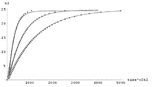
Figure 3: Solution for $h_{1}(t)$, $f_{h}=1$,$q_{2}=1$. Here $k_{2}/k_{1}=5$ and the three curves from left to right have $R_{M}=100,250,500$ respectively. The dots are plotted from the formula used to quasi-empirically fit the simulations in Ref. b2001

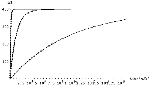
Figure 4: Solution for $h_{1}(t)$, $f_{h}=1$, $q_{2}=1$. Here $k_{2}/k_{1}=20$ and the three curves from left to right have $R_{M}=10^{7},10^{8},10^{9}$ respectively. The dots are plotted from the formula for used to quasi-empirically fit simulations of Ref. b2001

where $q_{2}=0$ in the above equations corresponds to $\beta(t)=\beta_{0}=$constant. and $q_{2}=1$ corresponds to $\beta(t)=\alpha(t)\beta_{0}/\alpha_{0}$. Solutions of these coupled equations are shown in Figs. 3-8, which are taken from fb . The key parameters are $k_{2}/k_{1}$, $R_{M}$, and $q_{2}$. In the figures, I have compared these results to the empirical fits of numerical simulations in b2001 . I used $h_{1}(t=0)=10^{-3}$, but the sensitivity to $h_{1}(0)$ is only logarithmic (see (61) below). In Fig. 1, $k_{2}/k_{1}=5$ was used, following B01, and in Fig. 2 $k_{2}/k_{1}=20$ was used.

In the figures, the solid lines represent numerical solutions to (54) and (55), whereas the dotted lines represent the formula given in b2001 , which is an empirical fit to simulation data assuming that $\alpha$ and $\beta$ are prescribed according to (58) and (59) below. More explicitly, Ref. b2001 found that the growth of $\overline{\bf B}$ was well described by the formula

$${B_{1}^{2}/B_{1,0}^{2}\over(1-B_{1}^{2}/B^{2}_{1,sat})^{1+{\alpha_{0}k_{1}-k_{1}^{2}\beta_{0}\over\nu_{M}k_{1}^{2}}}}=e^{2(\alpha_{0}k_{1}-k_{1}^{2}\beta_{0})t},$$ (56)

where $B_{1,0}=B_{1}(t=0)$. This can be rewritten using the notation above as a dimensionless equation for $t$ in units of $(k_{2}v_{2})^{-1}$, namely

$$t={k_{2}\over 2k_{1}}{{\rm Ln}[(h_{1}/h_{0})(1-h_{1}k_{1}^{2}/k_{2}^{2})^{R_{M}(k_{1}/k_{2}-2/3)-1}]\over{2/3}-{k_{1}/k_{2}}}.$$ (57)

Note that (56) and (57) correspond to $\alpha$ and $\beta$ quenching of the form

$$\alpha={\alpha_{0}\over 1+s_{B}B_{1}^{2}/v_{2}^{2}}$$ (58)

and

$$\beta={\beta_{0}\over 1+s_{B}B_{1}^{2}/v_{2}^{2}},$$ (59)

where $s_{B}\sim R_{M}(k_{1}/k_{2})(2/3-k_{1}/k_{2})=R_{M,2}(2/3-k_{1}/k_{2})$, and $R_{M,2}\equiv v_{2}/k_{2}\nu_{M}$. Eqns. (58) and (59) are derived from those in b2001 by re-scaling Eq. (55) of b2001 with the notation herein. It can also be shown directly that, up to terms of order $1/R_{M}$, (57) is consistent with that derived by substituting (58) and (59) into (54) and solving for $t$. Note that in contrast to the suggestion of b2001 , it is actually the forcing-scale magnetic Reynolds number, $R_{M,2}$, that plays a prominent role in these formulae.

The solutions of (54) and (55) are interesting. Insight can be gained by their sum

$$\partial_{t}h_{1}+\partial_{t}h_{2}=-{2\over R_{M}}\left({h_{1}k_{1}\over k_{2}}+{h_{2}k_{2}\over k_{1}}\right),$$ (60)

which corresponds to (51), the conservation of total magnetic helicity. If we make the astrophysically relevant assumption that $R_{M}>>1$, the right hand side of (51) is small for all $h_{1}$ and $h_{2}$. It follows that $\partial_{t}(h_{1}+h_{2})=0$ and for $h(t=0)=0$, this implies $h_{2}=-h_{1}$. In this period, we can self-consistently ignore $1/R_{M}$ in (54). If $q_{2}=1$, this phase ends when $h_{2}\rightarrow-1$, so that $h_{1}\sim 1$. This is manifested in figure 5.

This kinematic phase precedes the asymptotic saturation of the dynamo investigated by other authors, in which all time derivatives vanish exactly. For this to happen, the right hand side of (60) must vanish, which is equivalent to demanding that $h_{2}=-(k_{1}/k_{2})^{2}h_{1}$. Since the right hand sides of (54) and (55) are proportional to $1+h_{2}$ when terms of order $1/R_{M}$ are neglected, their vanishing requires that $h_{2}=-1$, and therefore, that $h_{1}=(k_{2}/k_{1})^{2}$. This is observed in figures 1 and 2. The asymptotic saturation (when the field growth ceases) takes a time of order $t_{sat}\sim R_{M}k_{2}/k_{1}$, which in astrophysics is often huge. Thus, although in principle it is correct that $\alpha$ is resistively limited (as seen from the solutions in figures 6 & 7) as suggested by vc ; ch ; gd1 ; by , this is less important than the fact that for a time $t_{kin}<R_{M}$ the kinematic value of $\alpha$ applies. The time scale $t_{kin}$ here is given by a few kinematic growth time scales for the $\alpha^{2}$ dynamo, more specifically,

$$t_{kin}\sim{\rm Ln}[1/h_{1}(0)](k_{2}/k_{1})/(4/3-2k_{1}/k_{2}).$$ (61)

For $h_{1}(0)=0.001$, $k_{2}/k_{1}=5$, $t_{kin}\sim 37$, as seen in Fig 5.

Note that $t_{kin}$ is sensitive to $k_{2}/k_{1}$ and independent of $R_{M}$. Figure 5 shows that there is significant disagreement in this regime with (58), but this formula was used in b2001 only to model the regime $t>R_{M}$, so the result is not unexpected. We can see from the solution for $\alpha$ itself that indeed the solutions of (54) and (55) do match (58) for $t>R_{M}$ (figures 6 and 7). Figure 6 shows the difference in the $\alpha$ along with (59) for the two values $R_{M}=10^{2}$ and $R_{M}=10^{3}$. Notice again the disagreement with the formula (58) until $t=R_{M}$, and agreement afterward. This marks the time at which the resistive term on the right of (54) becomes competitive with the terms involving $(1+h_{2})$. Asymptotic saturation does not occur until $t\sim t_{sat}=R_{M}k_{2}/k_{1}$ as described above.

Finally, note that $q_{2}=0$ corresponds to $\beta=\beta_{0}$. In general, this leads to a lower value of $h_{1}$ in the asymptotic saturation phase because this enforces zero saturation of $\beta$, whereas there is still some saturation of $\alpha$ in this limit. (Note that $q_{2}=0$ corresponds to the case of gd1 discussed in appendix B of fb .) For large $k_{2}/k_{1}$ the solutions of (54) and (55) are insensitive to $q_{2}=0$ or $q_{2}=1$. This is because the larger $k_{2}/k_{1}$, the smaller the influence of the $q_{2}$ terms in (54) and (55). This is highlighted in figure 8 where the result for $q_{2}=0$ is plotted with the b2001 fit. This suggests that for large-scale separation, the magnetic energy saturation is insensitive to the form of $\beta$ quenching. However, in real dynamos, magnetic flux and not just magnetic energy may be needed, so the insensitivity can be misleading because $\beta$ is needed to remove flux of the opposite sign. From the low $k_{2}/k_{1}$ cases, it is clear that that $q_{2}=1$ is a better fit to the simulations of b2001 .

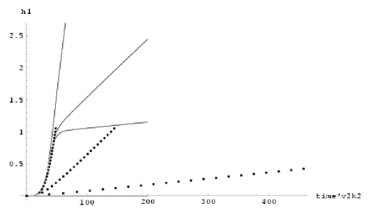
Figure 5: The early-time solution for $h_{1}(t)$, $f_{h}=1$, $q_{2}=1$. Here for $k_{2}/k_{1}=5$, and $R_{M}=10^{2},10^{3},10^{4}$ from left to right respectively. Notice the significant departure from the formula of b2001 at these early times. For $t<t_{kin}$ there is no dependence on $R_{M}$ and the growth proceeds kinematically.

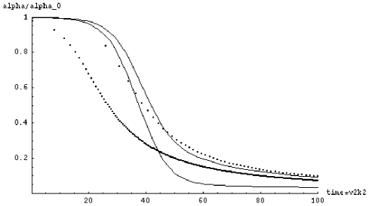
Figure 6: Solution of $\alpha/\alpha_{0}(t)$ for $h_{1}(t)$, $f_{h}=1$, $q_{2}=0$. Here $k_{2}/k_{1}=5$ and the solid lines are the solutions to (54) and (55) for $R_{M}=10^{2}$ (top curve) and $R_{M}=10^{3}$ (bottom curve) respectively. The top and bottom dotted curves are from (58), interpreted from Ref. b2001 . Notice the long kinematic phase for the solutions, the overshoot, and the convergence with that of (58) at $t=R_{M}$ for the $R_{M}=10^{2}$ case.

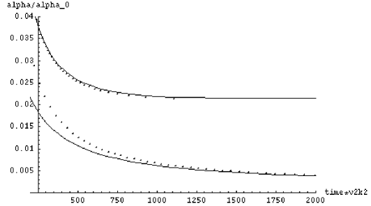
Figure 7: This is the extension of the previous figure for later times. Notice the convergence of the $R_{M}=10^{3}$ solution to (58) near $t=R_{M}$.

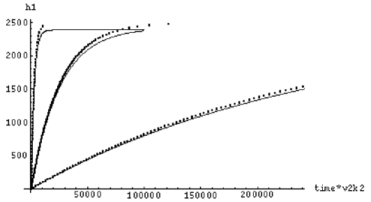
Figure 8: Solution for $h_{1}(t)$, $f_{h}=1$, $q_{2}=0$. Here $k_{2}/k_{1}=50$ and the three curves from left to right have $R_{M}=10^{2},10^{3},10^{4}$ respectively. The dotted lines are plotted from the formula used to quasi-empirically fit simulations of Ref. b2001 . For such large $k_{2}/k_{1}$ the fit to the data is only weakly sensitive to whether $q_{2}=1$ or $q_{2}=0$.

The physical picture of the quenching process just described is this: helical turbulence is forced at $k_{2}$ ($=5$ in b2001 ), and kept approximately constant by forcing. Hence $\alpha_{0}=-2\tau H^{V}_{2}/3={\it const}$. If $H_{1}^{M}$, the magnetic helicity at $k_{1}$ (which reaches $1$ here as a result of boundary conditions), is initially small — so that $|2k^{2}_{1}H^{M}_{1}/3|\ll|\alpha_{0}|$, (50) (or (54)) shows that it will be exponentially amplified provided that the damping due to $\beta+\lambda$ does not overcome the $\alpha$ effect. Initially, $\alpha=\alpha_{0}$, acting like a pump that moves magnetic helicity from $k_{2}$ to $k_{1}$ and driving the dynamo. This kinematic phase lasts until $t_{kin}$ as given by (61). Eventually, the growing $H^{M}_{1}$ results in a growing $H^{M}_{2}$ of opposite sign, which reduces $\alpha$ through $H^{C}_{2}$. $R_{M}$-dependent quenching kicks in at $t=t_{kin}$, but it is not until $t=R_{M}$ that the asymptotic formulae (58) and (59) are appropriate. Asymptotic saturation, defined by the time at which $B_{1}$ approaches its maximum possible value of $(k_{2}/k_{1})^{1/2}v_{2}$, occurs at $t=t_{sat}=R_{M}k_{2}/k_{1}$. For $t\geq R_{M}$ the numerical solution of (54) and (55), like the full numerical simulations of b2001 , is well fit by the $\alpha$ in (58) with a corresponding $\beta$ of (59). The two-scale approach is also consistent with B01 in that magnetic helicity jumps from $k_{2}$ to $k_{1}$ without filling in the intermediate wave numbers.

The emergence of the time scale $t_{kin}$ is interesting because it shows how one can misinterpret the implications of the asymptotic quenching formula (58) and (59). These formulae are appropriate only for $t>R_{M}$. The large-scale field actually grows kinematically up to a value $B_{1}=(k_{1}/k_{2})^{1/2}v_{2}$ by $t=t_{kin}$ and ultimately up to $B_{1}\sim(k_{2}/k_{1})^{1/2}v_{2}$ by $t=t_{sat}$. For large $R_{M,2}$, these values of $B_{1}$ are both much larger than the quantity $v_{2}/R_{M,2}^{1/2}$, which would have been inferred to be the saturation value if one assumed (58) and (59) were valid at all times.

Dynamical quenching or time-dependent approaches recognizing the current helicity as a contributor to $\alpha$ have been discussed elsewhere zeldovich ; kleeorinetal ; kleeorinruz ; kr (see also ji ), but here we have specifically linked the PFL $\alpha$ correction to the helicity conservation in a simple two-scale approach. Other quenching studies for closed systems such as ch and by advocated values of $\alpha$ which are resistively limited and of a form in agreement with (58) but with the assumption of a steady $B_{1}$. Assuming (53), and using (50) and (51) in the steady state, their formulae can be easily derived. However, one must also have a prescription for $\beta$. If $\beta$ is proportional to $\alpha$, then the resistively limited formulae like (25) emerges exactly, which is indeed approximately consistent with (58) and (59) for large $R_{M}$. If $\beta(t)=\beta_{0}$, as in gd1 , then a formula for $\alpha$ $without$ resistively limited quenching (24) emerges. On the other hand, fig. 8 shows that for large $k_{2}/k_{1}$, the dynamo quenching is largely insensitive to $\beta$.

Interestingly, if we cavalierly apply these results for the Galaxy (by incorrectly ignoring the shear and assuming an $\alpha^{2}$ dynamo that produces force free large scale fields), and use $k_{2}/k_{1}=20$, $B_{1}(0)=10^{-9}$, $v_{2}=10$km/s, and $k_{2}^{-1}\sim 100pc$, we would find the end of the kinematic regime to be at $t=140$, or about $1.4\times 10^{9}$yr. After this stage the field growth would proceed very slow because of the large $R_{M}$, but the saturation field strength at this time is $B_{1}\sim v_{2}/4.5$. Thus quite a large amplification can occur, even with an asymptotically slow dynamo. However this is really an academic exercise since for the Galaxy we need to consider an $\alpha-\Omega$ dynamo, and the boundary terms.

The generalized application of the principle that the magnetic helicity conservations should supplement the mean field dynamo growth equation to account for the backreaction is applied more generally to dynamos with shear in bb .

Finally, note that there is an important puzzle, hidden in the derivations here and those of gd1 ; by with regard to $\alpha$ quenching that we discuss in the next section.

2.4 Deriving $\alpha$ in Configuration Space: a Puzzle

The two-scale dynamical theory of section 2.3 fb for $\alpha$-quenching is appealing because it nicely couples the equations and concepts of magnetic helicity evolution to the current helicity contribution in $\alpha$, and fits simulation data well. The current helicity contribution was interpreted as a correction to the kinetic helicity contribution of kinematic theory. However, it depends on the current helicity contribution to $\alpha$ as presented in (52) being the total current helicity associated with $k_{2}$. To see what we mean by total and to show the complication, we consider the derivation of the turbulent EMF in configuration space.

The turbulent EMF can be written in three different ways:

$$\begin{array}[]{rcl}\langle{\bf v}\times{\bf b}\rangle=\langle{\bf v}(0)\times{\bf b}(0)\rangle+\int_{0}^{t}\langle\partial_{t^{\prime}}{\bf v}(t^{\prime})\times{\bf b}(t^{\prime})\rangle dt^{\prime}+\int_{0}^{t}\langle{\bf v}(t^{\prime})\times\partial_{t^{\prime}}{\bf b}(t^{\prime})\rangle dt^{\prime}\\ \\ =\langle{\bf v}(t)\times{\bf b}(0)\rangle+\int_{0}^{t}\langle{\bf v}(t)\times\partial_{t^{\prime}}{\bf b}(t^{\prime})\rangle dt^{\prime}\\ \\ =\langle{\bf v}(0)\times{\bf b}(t)\rangle+\int_{0}^{t}\langle\partial_{t^{\prime}}{\bf v}(t^{\prime})\times{\bf b}(t)\rangle dt^{\prime}\end{array}$$ (67)

The three lines in (67) simply correspond to the 3 relevant ways of using the formula $f(t)=f(0)+\int^{t}_{0}\partial_{t^{\prime}}f(t^{\prime})dt^{\prime}$, where $g$ is an arbitrary function of time. If I assume that $t>>0$, and that widely separated turbulent quantities do not correlate, the first terms on the right of the 2nd and 3rd lines respectively, can be dropped. We then have

$$\begin{array}[]{rcl}\langle{\bf v}\times{\bf b}\rangle=\int_{0}^{t}\langle{\bf v}(t)\times\partial_{t^{\prime}}{\bf b}(t^{\prime})\rangle dt^{\prime}=\int_{0}^{t}\langle\partial_{t^{\prime}}{\bf v}(t^{\prime})\times{\bf b}(t)\rangle dt^{\prime}.\end{array}$$ (69)

The second term in (69) as the standard textbook starting point moffatt ; krause for evaluating the turbulent EMF for a kinematic dynamo, but here I have not made any assumptions about the backreaction yet.

To illustrate the point, consider the simple case in which $\nabla\overline{\bf B}=0$. The equation for the small scale field is then

$$\begin{array}[]{r}\partial_{t^{\prime}}{\bf b}=\overline{\bf B}\cdot\nabla{\bf v}+{\bf b}\cdot\nabla{\bf v}-{\bf v}\cdot\nabla{\bf b}-\nabla\times\langle{\bf v}\times{\bf b}\rangle+\nu_{M}\nabla^{2}{\bf b}.\end{array}$$ (70)

The penultimate term goes away when included in (69) and we ignore the last term. The first terms on the right, upon the assumption that the dominant contributions to correlations are isotropic in ${\bf v}$, gives the “textbook” expression for $\alpha$ plus extra terms, that is

$$\langle{\bf v}\times{\bf b}\rangle\simeq-{\overline{\bf B}\over 3}\int_{0}^{t}\langle{\bf v}(t)\cdot\nabla\times{\bf v}(t^{\prime})\rangle dt^{\prime}+Q(v^{2}b).$$ (71)

The terms symbolized by $Q(v^{2}b)$ are typically ignored using some version of the first order smoothing approximation. This is of questionable validity, given that the small scale field rapidly grows to exceed the mean field. We will come back to the relevance of these terms below.

Now if instead I use the last term of (69) to expand the EMF, I must then invoke the Navier-Stokes equation for the time derivative of the turbulent velocity

$$\partial_{t}{{\bf v}}=-{\bf v}\cdot\nabla{\bf v}-\langle{\bf v}\cdot\nabla{\bf v}\rangle-\nabla p_{eff}+{\overline{\bf B}}\cdot\nabla{\bf b}+{\bf b}\cdot\nabla{\bf b}-\langle{\bf b}\cdot\nabla{\bf b}\rangle+\nu\nabla^{2}{\bf v}+{\bf f}({\bf x},t),$$ (72)

where $\bf f$ is a forcing function and $p_{eff}$ is the magnetic and thermal pressure. Upon plugging this into (69), the second and sixth terms on the right vanish. If we ignore the viscosity, and assume the dominant contribution to correlations are isotropic, we then have

$$\langle{\bf v}\times{\bf b}\rangle\simeq{\overline{\bf B}\over 3}\int_{0}^{t}\langle{\bf b}(t)\cdot\nabla\times{\bf b}(t^{\prime})\rangle dt^{\prime}+{\tilde{Q}}(v^{2}b,fb)$$ (73)

Notice two things about (71) and (73): First they are equal to each other since they were derived from different choices of the expansion of $\langle{\bf v}\times{\bf b}\rangle$. Second, they do not cleanly include the combination of the total residual helicity, required in (52) when placed into (50) and (51) to derive (54) and (55). The only way that (71) and (73) can have the form of the desired relative helicity is if $Q(v^{2}b)={\overline{\bf B}\over 3}\int_{0}^{t}\langle{\bf b}(t)\cdot\nabla\times{\bf b}(t^{\prime})\rangle dt^{\prime}$ and if ${\tilde{Q}}(v^{2}b,fb)=-{\overline{\bf B}\over 3}\int_{0}^{t}\langle{\bf v}(t)\cdot\nabla\times{\bf v}(t^{\prime})\rangle dt^{\prime}$. I have been unable to prove that this is the case for the astrophysically relevant weak $\bar{B}$ regime.

There is another approach to calculating the EMF in configuration space that does reveal a similar difference of helicities as that in (52), namely the approach of fbc . But ${\bf v}$ and ${\bf b}$ enter (52) whereas ${\bf v}^{(0)}$ and ${\bf b}^{(0)}$, the statistically isotropic parts of ${\bf v}$ and ${\bf b}$, enter fbc . To see this more explicitly, I write

$${\bf v}={\bf v}^{(0)}+{\bf v}^{(A)},$$ (74)

where $A$ indicates an anisotropic contribution, the result of the backreaction from $\overline{\bf B}$. Similarly,

$${\bf b}={\bf b}^{(0)}+{\bf b}^{(A)}.$$ (75)

(Even when ${\bf b}$ is the result of stirring up an initial seed $\overline{\bf B}$, there is still a ${\bf b}^{(0)}$ which is the statistically isotropic part of ${\bf b}$.) We then assume that the statistics of the zeroth order turbulent correlations are those of a homogeneous isotropic, “known” base state. The goal is to express turbulent correlations in terms of the zeroth order quantities. It is sufficient to demonstrate the basic idea invoked to all orders in $\overline{\bf B}$ in fbc with that derived to linear order in bf99 Noting that $\langle{\bf v}\times{\bf b}\rangle^{(0)}$ vanishes, the lowest order contribution to the turbulent EMF is

$$\begin{array}[]{rcl}\langle{\bf v}\times{\bf b}\rangle^{(1)}=\langle{\bf v}^{(0)}\times{\bf b}^{(1)}\rangle+\langle{\bf v}^{(1)}\times{\bf b}^{(0)}\rangle\\ =\int^{t}_{0}\langle{\bf v}^{(0)}(t)\times\partial_{t^{\prime}}{\bf b}^{(1)}(t^{\prime})\rangle dt^{\prime}+\int^{t}_{0}\langle\partial_{t^{\prime}}{\bf v}^{(1)}(t^{\prime})\times{\bf b}^{(0)}(t)\rangle dt^{\prime}\end{array}$$ (78)

To linear order, using the induction equation for ${\bf b}^{(1)}$ and the Navier-Stokes equation for ${\bf v}^{(1)}$, it can be shown that by analogy to the derivations of (71) and (73), (combined with a revised first order smoothing approximation that assumes $|{\bf b}^{(1)}/\overline{\bf B}|<1$) (78) becomes

$$\langle{\bf v}\times{\bf b}\rangle^{(1)}=-{\overline{\bf B}\over 3}\left(\int^{t}_{0}\langle{\bf v}^{(0)}(t)\cdot\nabla\times{\bf v}^{(0)}(t^{\prime})\rangle dt^{\prime}-\int^{t}_{0}\langle{\bf b}^{(0)}(t)\cdot\nabla\times{\bf b}^{(0)}(t^{\prime})\rangle dt^{\prime}\right).$$ (79)

FBC showed that in the case of negligible mean field gradients, it is still the zeroth order kinetic and current helicities which appear most explicitly in $\alpha$, even to all orders in $\overline{\bf B}$.

It is clear that the zeroth order helicities are not necessarily equal to those constructed with the full turbulent quantities since

$$\langle{\bf v}\cdot\nabla\times{\bf v}\rangle=\langle{\bf v}^{(0)}\cdot\nabla\times{\bf v}^{(0)}\rangle+\langle{\bf v}^{(A)}\cdot\nabla\times{\bf v}^{(0)}\rangle+\langle{\bf v}^{(A)}\cdot\nabla\times{\bf v}^{(0)}\rangle$$ (80)

and similarly

$$\langle{\bf b}\cdot\nabla\times{\bf b}\rangle=\langle{\bf b}^{(0)}\cdot\nabla\times{\bf b}^{(0)}\rangle+\langle{\bf b}^{(A)}\cdot\nabla\times{\bf b}^{(0)}\rangle+\langle{\bf b}^{(A)}\cdot\nabla\times{\bf b}^{(0)}\rangle,$$ (81)

so the extra terms on the right must be dealt with. One might ask however, if the first terms on the right of (80) and (81) dominate, why can’t we simply replace $\langle{\bf b}^{(0)}\cdot\nabla\times{\bf b}^{(0)}\rangle$ by $\langle{\bf b}\cdot\nabla\times{\bf b}\rangle$ wherever the former occurs? The reason is that the appropriate helicity which then enters $\alpha$ is $\langle{\bf b}^{(0)}\cdot\nabla\times{\bf b}^{(0)}\rangle$ to lowest order. Then the $H_{1}^{M}$ entering on the left of (50) would be second order. But then the magnetic helicity, $H_{2}^{M}$, entering (51) would also be second order. Thus the current helicity entering $\alpha$ is zeroth order whereas that entering the helicity conservation equation would be second order. There is an ordering mismatch. This is a problem because the success of the model of 2.3 depends on our being able to circumvent this ordering ambiguity and presume that the current helicity entering (52) is exactly $k_{2}^{2}$ times the $H_{2}^{M}$ entering (51).

The procedure outlined to derive (79) and the subtlety just described with respect to ordering is basically the “ordering ambiguity” that was discussed in bf99 . There it was shown that Refs. gd1 ; by effectively derived the form (78) rather than (52) by linearizing in terms of $\overline{\bf B}$ but did not identify that they had derived the zeroth order contribution to $\alpha$. Thus Refs. gd1 ; by were actually using a similar expansion to that of fbc . The subsequent manipulations of gd1 and by required that they had derived $\alpha$ as a function of the full ${\bf v}$ and ${\bf b}$, much like our manipulations in section 2.3. The issue also arises subtly in the $k$ space derivation of PFL and is presently unresolved.

3 Conclusions and Open Questions

3.1 Small Scale Dynamo

For non-helical turbulence, and for $Pr\geq 1$, current simulations indicate that the magnetic field piles up on the resistive scales $k>>k_{f}$ when forced externally maroncowley in a periodic box. The reason for this effect seems to be that the forcing scale inputs shear directly into the small scale fields, so the power on small scales is the result of cross field structure. But for sufficiently helical turbulence, the spectrum changes: the peak at the resistive scale migrates to the forcing scale (wavenumber $k_{f}$) maronblackman . Can we understand the migration of the small scale field peak as a function of time? Will this picture survive future numerical testing? How do the boundary conditions affect the results?

To explain the change in the small-scale spectrum from the non-helical to helical case, it is possible that what works for the large scale field may also help understand what happens for the small scale field. The kinetic helicity input at $k_{f}$ also cascades to higher wavenumbers, and so there is a source of helicity at these wavenumbers. Perhaps the change in shape of the small scale spectrum might be modeled by a self-similar set of nested “mean-field” dynamos. The principle is that for each small scale wavenumber $k_{s}>k_{f}$ there is a range of $k_{f}<k_{l}<k_{s}$ for which of inverse cascade field growth driven by the helical turbulence at $k_{s}$ can overcome the forward cascade of magnetic energy to $k>k_{l}$. An inverse cascade modeled in this way might account for the overall spectral shape change, but this is presently just speculation.

3.2 Large Scale Periodic Box $\alpha^{2}$ Dynamo

The critical value of fractional helicity which determines the migration of the small scale peak is exactly the same as that for which the kinematic $\alpha^{2}$ dynamo has a positive growth rate, and so a large scale field grows at $k_{1}<k_{f}$ in concurrence with the migration of the small scale peak to $k_{f}$ (see section 1 and 4). The rate of growth, the saturation level, and the dependence on $R_{M}$ observed in periodic box simulations of fully non-linear $\alpha^{2}$ dynamo seem to be well modeled by a two-scale dynamical quenching model of Ref. fb and section 4. The dynamo $\alpha$ is the difference between the kinetic and current helicities associated with the small scale field, and the growth of the large scale field is associated with the growth of the large scale magnetic helicity. Because total magnetic helicity is conserved up to a resistive term, the growth of large scale magnetic helicity also means growth of the opposite sign of small scale magnetic helicity, and thus small scale current helicity. This eventually suppresses the growth of the large scale magnetic field by reducing $\alpha$. The time dependent process is non-linear. There are some unresolved issues with this theory however: 1) the theory works well for maximally helical forcing. How does it generalize to arbitrary helical forcing? 2) How is the correction to $\alpha$ to be properly derived in configuration space (see section 5.)? The success of the theory is based on the formula of $\alpha$ from pfl which leaves open the ordering ambiguity discussed in section 5. 3) What is the appropriate theory for $\beta$ quenching? The saturation value of the mean field in the $\alpha^{2}$ dynamo depends somewhat on the choice of $\beta$ but the ratio of large to small scale fields does not. Dynamos with shear and their cycle periods are sensitive to the form of $\beta$ bb . 4) Along these lines, how does the dynamical quenching theory based on magnetic helicity conservation apply to the $\alpha-\Omega$ dynamo? This is work in progress bb . 5) Do dynamos in astrophysics really need to be fast? This is another important reason to study $\beta$ quenching. But the question should be revisited. Perhaps the kinematic phase (see (61)) can last long enough for substantial amplification, even for asymptotically slow dynamos when no cycle period is required. But one must also consider the observed cycle periods like that of the sun which seem to be fast. Perhaps highly anisotropic turbulence and small cross field structures that can dissipate quickly might even allow fast cycle periods with through redefined $R_{M}$. See also brannach .

3.3 Coronal Activity and Open Boundary Dynamos (OBD)

In addition to these considerations, the role of boundary terms needs to be considered. In a real system there is gravity, rotation, shear, stratification and buoyancy. It may not be enough to just invoke arbitrarily open boundaries to test the OBD but the physics at the boundary itself needs to be studied (e.g. rafikov ). Winds might be essential. Do mean field dynamos act in symbiosis with jets and winds? We know that the sun is shedding magnetic helicity. Does this enable the mean field dynamo to be fast for all times? In astrophysical rotators, the $\alpha$ effect should depend on height. How does this enter in the non-linear theory?

I showed above that the estimated energy deposition rates to maintain fast mean field dynamo action are consistent with the coronal + wind power from the Sun, Galaxy and Seyfert I AGN all of these sources are natural sites for $\alpha-\Omega$ type dynamos. The helical properties also seem to agree well in the solar case where they can be observed rustkumar . The steady flow of magnetic energy into coronae thus provides an interesting connection between mean field dynamos and coronal dissipation in a range of sources. A reasonably steady (over time scales long compared to turbulent turnover time scales), active corona with multi-scale helical structures, may provide a self-consistency check for fast dynamo production of magnetic field.

For the $\alpha^{2}$ case, figure 9 shows the effect of including an additional loss term in (55), proportional to $h_{2}$, on the growth of $h_{1}$. The effect is to suppress the backreaction by taking away excess small scale helicity and allowing the large scale field to grow stronger. Understanding appropriate form of loss term for real $\alpha-\Omega$ dynamos needs more study.

3.4 New Diagram of MFD Operation is Needed

Related to the boundary issue is the generation of magnetic flux inside of a rotator. For the Galaxy, diffusion of $\overline{\bf B}$ at the boundary is required to maintain a quadrapole field structure with a net flux inside the disk parker . The total flux is conserved, but to obtain a net flux inside the rotator where desired, the return flux must be shed from this region. The surface diffusion of total magnetic field for the Galaxy may be difficult rafikov and remains an open question. (One alternative possibility is that the mean field diffuses radially more efficiently at the top of the disk than at the mid-plane.) Note however, that it is $\overline{\bf B}$ which needs to diffuse, not necessarily the total field or the matter. For the Sun, the solar cycle also requires diffusion of mean field through the boundary at the surface and/or mid-plane.

Since both flux generation inside the rotator, and helicity shedding can both appeal to boundary terms it is possible that the two are related in the simplest $\alpha-\Omega$ dynamo. Note that it was the growth of the small scale $current$ helicity $\langle{\bf j}\cdot{\bf b}\rangle$ that leads to the suppression of $\alpha$. Thus one can ask directly if the textbook $\alpha-\Omega$ dynamo has any way of getting rid of this quantity and at the same time generating magnetic flux.

In fact there there is something missing when one draws a standard picture of dynamo action either for $\alpha^{2}$ or for $\alpha-\Omega$. The latter is shown in figure 10, but the implication holds also shown for the $\alpha^{2}$ case. The issue is that the small scale loop that arises from the kinetic part of the $\alpha$ effect actually induces the $same$ sign of the current helicity of the small scale field as that of the large scale field that it generates. But I have discussed how the growth of the large scale field should be accompanied by the $opposite$ sign of the small scale helicities. It is intriguing because in the kinematic regime of the $\alpha^{2}$ dynamo, the small scale field does grow first at the smallest scales, and it seems to take nearly until $t_{kin}$ for the peak of the current helicity of opposite sign to the large scale to move fully up to the forcing scale (Brandenburg and Maron, personal communication.) In this sense, figure 10 seems limited to the kinematic regime: it would be nice to see a more accurate picture that actually shows the generation of the small scale current helicity of opposite sign to that of the large scale and how it migrates to the forcing scale graphically.

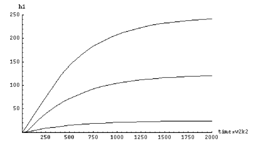
Figure 9: The effect of a adding a loss term proportional to $h_{2}$ in (55) on the growth of $h_{1}$ for three different values of loss. The loss term is added by introducing multiplicative factors on the last term of (55). From top to bottom, these factors are $10,5$ and $1$(=no loss), respectively. Here $R_{M}=200$ and $k_{2}/k_{1}=5$.

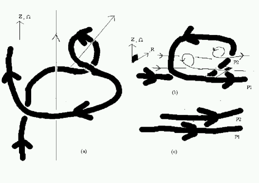
Figure 10: The kinematic picture and its limitations. This is assumed to be a northern hemisphere so that kinetic helicity is negative. (a) The large scale loop results from shear and the small loop results from the $\alpha$ effect. Note that the current helicity of the smaller loop has the same sign as that of the large scale loop. So the question arises: in a revised picture how can one incorporate the growth of magnetic and/or current helicity of the opposite sign that accompanies growth of large scale helicity? (b) This just shows the effect of multiple small scale loops as they sum together. (c) the process of reinforcement of the toroidal field is shown.

Finally, note that it is in part the potential for flux generation that distinguishes a mean field dynamo from the kind of dynamo which generates large scale fields as a result of the magneto-rotational instability (MRI). There, the field induces turbulence, which then generates a random component of the field, which is subsequently sheared by the differential rotation. Magnetic energy grows exponentially, even on the largest scale allowed, but there is no real flux generation here and no need for input helicity. Note however that for real accretion discs, helicity is undoubtedly present since all the ingredients are there, density gradient, and turbulence. Thus it is important to understand even in accretion disks, what is the role of helical dynamos. This has not yet been done exhaustively. From this point of view, the mean field dynamo formalism should still apply, with a dynamical theory for quenching, and the MRI may play the role as the source of turbulence. Nevertheless more work is needed.

3.5 What is the Role of Magnetic Reconnection?

It is generally perceived that reconnection is important for large scale dynamos but the precise way in which this is the case is subtle. In general, the processes of reconnection can serve two roles: it changes the topology of the field, and also dissipates magnetic energy. In the mean field dynamo formalism, the large scale field is degenerate with respect to small scale topology. By definition, taking the mean means smoothing out over the small scales. Thus a series of disconnected loops could have the same mean field as an undulating topologically connected field. In the mean field formalism therefore, the role of reconnection is not explicit.

Neither the mean field nor the fluctuating field are the actual field. If one really does want the mean field dynamo to result in a topologically connected actual field, then reconnection would be important for the topology. But it is important to asses the particular application for when this is necessary: the large scale field in the Galaxy is measured mainly by Faraday rotation which provides little information about the actual field topology. The role of reconnection may only be one of ensuring that there is a turbulent cascade which ensures that heat rather than the magnetic field is sink of the kinetic energy.

Another unanswered question relating to dynamos and reconnection is: does reconnection play in the conservation of magnetic helicity and in the migration of the peak of the small scale magnetic energy from the resistive scale to the forcing scale in helically forced turbulence?

Acknowledgments:

Thanks to the organizers (E. Falgarone and T. Passot) of the Paris May 2001 workshop on MHD turbulence for an excellent meeting. Thanks to G. Field, A. Brandenburg, and J. Maron for recent collaborations incorporated into the material herein. Thanks also to R. Kulsrud, B. Mattheaus, and A. Pouquet for stimulating discussions. Support from DOE grant DE-FG02-00ER54600 is acknowledged.

References

- (1) A.A. Ruzmaikin, A.M. Shukurov, D.D. Sokoloff, Magnetic Fields of Galaxies, (Kluwer Press, Dodrecht, 1988).
- (2) R. Kulsrud, R. Cen, J.P. Ostriker, and D. Ryu, ApJ, 480 481 (1997)
- (3) E. G. Zweibel & C. Heiles, Nature, 385 131 (1997).
- (4) B.D.G. Chandran, S.C. Cowley, & M. Morris, ApJ, 528 723 (2000).
- (5) S.H. Lubow, J.C.B. Papaloizou, J.E. Pringle, MNRAS, 267, 235 (1994).
- (6) A.P. Kazanstev, Sov. Physics. JETP, 26 1031 (1968).
- (7) E.N. Parker, Cosmical Magnetic Fields (Oxford: Clarendon Press, 1979).
- (8) Ya. B. Zeldovich , A.A. Ruzmaikin, , and D.D. Sokoloff, Magnetic Fields in Astrophysics, (Gordon and Breach, New York, 1983).
- (9) R.M. Kulsrud & S.W. Anderson, Astrophys. J. 396 606 (1992).
- (10) S. Kida, S. Yanase, J. & Mizushima, Physics of Fluids, 3 457 (1991)
- (11) J. Maron & S. Cowley, to be submitted to ApJ (2002); http://xxx.lanl.gov/abs/astro-ph/0111008
- (12) A. Schekochihin, S. Cowley, J. Maron, J., & L. Malyshkin 2002, Phys Rev. E., 65, 6305.
- (13) R. Beck., A. Brandenburg, D. Moss, A. Shukurov, D. Sokoloff, Galactic Magnetism: Recent Developments and Perspectives, Ann. Rev. Astron. Astrophys., 34, 155 (1996).
- (14) J. Maron & E.G. Blackman, ApJL 566, L41 (2002).
- (15) E. Vishniac & J. Cho, ApJ, 550 752 (2000).
- (16) A. Brandenburg, ApJ, 550 824 (2001)
- (17) H.K. Moffatt, H. K. Magnetic Field Generation in Electrically Conducting Fluids, (Cambridge University Press, Cambridge, 1978).
- (18) F. Krause & K.-H. Rädler Mean-field magnetohydrodynamics and dynamo theory, (Pergamon Press, New York, 1980).
- (19) M. Steenbeck, F. Krause, & K.-H. Rädler, Z. Naturforsch. 21a, 369 (1966).
- (20) S.A. Balbus & J. Hawley , Rev. Mod. Phys. 70, 1 (1998).
- (21) T.G. Cowling, Magnetohydrodynamics, (Wiley Interscience, New York, 1957).
- (22) J.H. Piddington, Cosmical Electrodynamics, (Krieger Press, Malbar, 1981).
- (23) S.I. Vainshtein & F. Cattaneo, ApJ 393 165 (1992).
- (24) L.L. Kitchatinov, V.V. Pipin, G. Rüdiger, G., & M. Kuker, Astron. Nachr., 315, 157 (1994).
- (25) F. Cattaneo, & D.W. Hughes, Phys. Rev. E. 54, 4532 (1996).
- (26) E.G. Blackman & A. Brandenburg, submitted to ApJ (2002); http://xxx.lanl.gov/abs/astro-ph/0204497.
- (27) S. Vainshtein, Phys. Rev. Lett., 80, 4879 (1998).
- (28) A. Brandenburg, W. Dobler, & K. Subramanian, Astron. Nachr, 323 99 (2002).
- (29) A. Brandenburg, A. Bigazzi, & K. Subramanian, MNRAS 325 685 (2001)
- (30) G.B. Field & E.G. Blackman, in press ApJ, xxx.lanl.gov/abs/astro-ph/0111470, (2002).
- (31) A. Pouquet, U. Frisch, & J. Leorat, J. Fluid Mech. 77, 321 (1976).
- (32) G.B. Field in Magnetospheric Phenomena in Astrophysics, R. Epstein & W. Feldman, eds. AIP Conference Proceedings 144 (American Institute of Physics, Mellville NY, 1986), p324.
- (33) E.G. Blackman, & G.B. Field, Astrophys. J. 534 984 (2000a).
- (34) M.A. Berger & G.B. Field, J. Fluid Mech. 147 133 (1984).
- (35) J.W. Bieber & D.M. Rust, ApJ, 453 911 (1995)
- (36) D.M. Rust & A. Kumar , Astrophys. J. 464, L199 (1994).
- (37) J.A. Markiel & J.H. Thomas, Astrophys. J. 523 827 (1999)
- (38) A. Ruzmaikin, in Magnetic Helicity in Space and Laboratory Plasmas, edited by A. Pevtsov, R. Canfield, & X. Brown, (Amer. Geophys. Union, Washington, 1999), p111; M.A. Berger & A. Ruzmaikin, Journ. Geophys. Res. 105, 110481
- (39) U. Frisch, A. Pouquet, J. Léorat & A. Mazure, J. Fluid Mech. 68, 769 (1975).
- (40) G.L. Withbroe, & R.W. Noyes, Ann. Rev. Astron. Astrophys. 15, 363 (1977);
- (41) E.G. Blackman, & G.B. Field, Mon. Not. R. Astron. Soc. 318, 724 (2000a).
- (42) B.D. Savage, in The Physics of the Interstellar Medium and Intergalactic Medium, A. Ferrara, C.F. McKee, C. Heiles, & P.R. Shapiro eds. ASP conf ser vol 60. (Astronomical Society of the Pacific, San Francisco, 1995), p233.
- (43) R.J. Reynolds, L.M. Haffner, S.L. Tufte , Astrophys. J. 525, L21 (1999).
- (44) M. DeVries & J. Kuijpers, Astron. & Astrophys. 266, 77 (1992); F. Haardt & L. Maraschi, Astrophys. J. 413, 507 (1993); G.B. Field & R.D. Rogers., Astrophys. J. 403, 94 (1993); T. DiMatteo E.G. Blackman & A.C. Fabian, Mon. Not. R. Astron. Soc. 291 L23 (1997); A. Merloni & A.C. Fabian, accepted to Mon. Not. R. Astron. Soc. astro-ph/0009498 (2000);
- (45) H. Ji, Phys. Rev. Lett. 83 3198 (1999); H. Ji in Magnetic Helicity in Space and Laboratory Plasmas, edited by A. Pevtsov, R. Canfield, & X. Brown, (Amer. Geophys. Union, Washington, 1999), p167; H. Ji, & Prager, S. C. in press Magnetohydrodynamics, astro-ph/0110352 (2001)
- (46) A.V. Gruzinov & P.H. Diamond P.H., Phys. Rev. Lett., 72 1651 (1994); A.V. Gruzinov & P.H. Diamond, Physics of Plasmas, 2 1941 (1995);
- (47) A.V. Gruzinov & P.H. Diamond, Physics of Plasmas, 3 1853 (1996).
- (48) A. Bhattacharjee & Y. Yuan, Astrophys. J. 449 739 (1995).
- (49) N. Kleeorin, D. Moss, D., I. Rogachevskii, D. Sokoloff, A&A, 361 L5 (2000)
- (50) N. Kleeorin, I. Rogachevskii, A. Ruzmaikin, A&A, 297 L59 (1995)
- (51) N. Kleeorin & I. Rogachevskii, Phys. Rev. E., 59 6724 (1999)
- (52) G.B. Field, E.G. Blackman, & H. Chou, Astrophys. J. 513, 638 (1999).
- (53) Ya.-B. Zeldovich, Sov Phys. JETP, 4 460 (1957).
- (54) E.G. Blackman and G.B. Field, Physics of Plasmas, 8 2407 (2001)
- (55) E.G. Blackman & G.B. Field, Astrophys. J. 521 597 (1999).
- (56) W.N. Brandt, T. Boller, A.C. Fabian,& M. Ruszkowski, Mon. Not. R. Astron. Soc. 303, L53 (1999).
- (57) R.R. Rafikov& R.M. Kulsrud, Mon. Not. R. Astron. Soc. 314, 839 (2000).
- (58) F. Cattaneo, Astrophys. J. 434, 200 (1994).
- (59) A. Brandenburg, & W.Dobler A&A, 369 329 (2001).
- (60) R. Arlt & A. Brandenburg A&A 380, 359 (2001)