Quintessence, super-quintessence and observable quantities in Brans-Dicke and non-minimally coupled theories

Abstract

The different definitions for the equation of state of a non-minimally coupled scalar field that have been introduced in the literature are analyzed. Particular emphasis is made upon those features that could yield to an observable way of distinguishing non-minimally coupled theories from General Relativity, with the same or with alternate potentials. It is found that some earlier claims on that super-quintessence, a stage of super-accelerated expansion of the universe, is possible within realistic non-minimally coupled theories are the result of an arguable definition of the equation of state. In particular, it is shown that these previous results do not import any observable consequence, i.e. that the theories are observationally identical to General Relativity models and that super-quintessence is not more than a mathematical outcome. Finally, in the case of non-minimally coupled theories with coupling $F=1+\xi\phi^{2}$ and tracking potentials, it is shown that no super-quintessence is possible.

I Introduction

During the last years, observations of distant Type Ia supernovae 1 and CMB measurements 2 have shown that the universe is, most likely, undergoing a process of accelerated expansion. The widespread vision of the cosmological model is, since then, a spatially flat low matter density universe. This implies that the total energy density today is dominated by a contribution having negative pressure (cosmological constant, or quintessence Q ) which has just began to undertake the leading role in the right hand side of the Einstein field equations.

The cosmological constant solution to this state of affairs appears not to be completely satisfactory (see for instance 3 ). Precise initial conditions should be given in order to solve the coincidence problem (why the vacuum energy is dominating the energy density right now). Moreover, a fine-tuning problem appears, since a vacuum energy density of order $\sim 10^{-47}{\rm GeV}^{4}$ requires a new mass scale about 14 orders of magnitude smaller than the electroweak scale, having no a-priori reason to exist. In addition, the equation of state, $p/\rho$, for vacuum energy is exactly equal to $-1$, what at first sight appears as yet another value which is, in a dynamical setting, precisely set. Quintessence Q , and its derived models, being the main alternatives, are based on the existence of one or many scalar fields, which dynamically evolve together with all others components of the universe. The above-mentioned problems are alleviated within this framework. A sub-class of models, those having inverse power law potentials, present tracking solutions where a given amount of scalar field energy density can be reached starting from a large range of initial conditions (see for e.g. Refs. tracking ).

The simplest models of quintessence are based on minimally coupled scalar fields. For a general potential $V$, the equation of state for those quintessence models is given by

$$\frac{p}{\rho}=\frac{\dot{\phi}^{2}-2V}{\dot{\phi}^{2}+2V},$$ (1)

and it can be easily proven that this expression is bounded to be within the range -1 $\leq p/\rho\leq$ 1, unless of course one is willing to accept negative defined potentials. In the latter cases, the energy density becomes itself a negative quantity. For usual models of quintessence, then, it is clear that no super-acceleration can appear. The latter is a result of an extremely negative ($<-1$) equation of state. This possible super-accelerated expansion has been recently dubbed super-quintessence by several authors, e.g. faraoni , although its consequences are being analyzed since some time before menace . The main reason supporting this interest is that current observational constraints are indeed compatible with, if not favoring, such values for the equation of state (see for instance Ref. menace ).

Extended quintessence models are those in which the underlying theory of gravity contains a non-minimally coupled scalar field. It is this same scalar field which, apart from participating in the gravity sector of the theory, is enhanced by a potential to fulfill the role of normal quintessence. From a theoretically point of view, these ideas are appealing: it is the theory of gravity itself what provides the dynamically evolving, and currently dominating, field. Recent works on this area include those presented in Refs. faraoni ; Sen ; perrota ; per2 ; uzan ; farese ; chiba . We will have the opportunity to comment with much more detail on some of these works below. In addition, just to quote a few others in a so vastly covered topic, see the works of Ref. new . We would also like to remark that one of the first detailed analysis of a non-minimally coupled theory with a scalar field potential was made by Santos and Gregory santos , years before the concept of quintessence was introduced.

It has been claimed by many that a non-minimally coupled theory, like for instance Brans-Dicke gravity, can harbor super-quintessence solutions (e.g. faraoni ; Sen ). However, there are different, and in most cases conflicting, definitions for the equation of state in these theories. Then, care should be exercised when analyzing the claims of the existence of super-quintessence solutions: in some cases, they do not report either any physical import, because the equation of state really is not more than a complex relationship between the field and its derivative without any supporting conservation law, nor any observational consequence, because the amount of super-quintessence is so small that is far beyond any foreseen experiment. It is the aim of this paper to help in clarifying these points, and to analyze, from an observational point of view, how non-minimally coupled theories differentiate from usual General Relativity in what concerns to quintessence and super-quintessence models.

The rest of this work is presented as follows. In the following Section we comment on the energy conditions and the status of super-quintessence regarding them. Then, we introduce the gravity theories we are interested in. Section IV analyzes the case of Brans-Dicke gravity whereas Section V studies more general non-minimally coupled theories. A discussion and summary of the results is given in Section VI. A brief Appendix discusses an alternative formulation of the theories of gravity, useful for numerical computations.

II The energy conditions

For a Friedman-Robertson-Walker space-time and a diagonal stress-energy tensor $T_{\mu\nu}=(\rho,-p,-p,-p)$ with $\rho$ being the energy density and $p$ the pressure of the fluid, the energy conditions (EC) read:

null: NEC $$\iff (\rho+p\geq 0),$$

weak: WEC $$\iff (\rho\geq 0)\hbox{ and }(\rho+p\geq 0),$$

strong: SEC $$\iff (\rho+3p\geq 0)\hbox{ and }(\rho+p\geq 0),$$

dominant: DEC $$\iff (\rho\geq 0)\hbox{ and }(\rho\pm p\geq 0).$$ (2)

They are, then, linear relationships between the energy density and the pressure of the matter/fields generating the space-time curvature. Violations of the EC have sometimes been presented as only being produced by unphysical stress-energy tensors. If NEC is violated, and then WEC is violated as well, negative energy densities –and so negative masses– are thus physically admitted. However, although the EC are widely used to prove theorems concerning singularities and black hole thermodynamics, such as the area increase theorem, the topological censorship theorem, and the singularity theorem of stellar collapse VISSER-BOOK , they lack a rigorous proof from fundamental principles. Moreover, several situations in which they are violated are known; perhaps the most quoted being the Casimir effect, see for instance Refs. VISSER-BOOK ; last-visser for additional discussion. Observed violations are produced by small quantum systems, resulting of the order of $\hbar$. It is currently far from clear whether there could be macroscopic quantities of such an exotic, e.g. WEC-violating, matter/fields may exist in the universe. A program for imposing observational bounds (basically using gravitational micro and macrolensing) on the existence of matter violating some of the EC conditions has been already initiated, and experiments are beginning to actively search for the predicted signatures obs . Wormhole solutions to the Einstein field equations, extensively studied in the last decade (see Refs. VISSER-BOOK ; wh for particular examples), violate the energy conditions, particularly NEC. Wormholes are probably the most interesting physical entity that could exist out of a macroscopic violation of the EC.

It is interesting to analyze what does super-quintessence imply concerning the validity of the EC. As stated in the Introduction, super-quintessence is described by a cosmic equation of state

$$\frac{p}{\rho}<-1,$$ (3)

and so different situations arise depending on the sign of the energy density $\rho$. If $\rho>0$, super-quintessence implies $p+\rho<0$, and thus the violation of all the point-wise EC quoted above. Note that WEC is violated because of the violation of its second inequality. If, on the contrary, already $\rho<0$, then NEC may be sustained, but WEC is violated. Super-quintessence then implies strong violations of the commonly cherished EC. But, should this be taken as sufficiently unphysical as to discard a priori the possibility of a super-accelerating phase of the universe?

Apart from the finally relevant response, coming from experiments (today super-quintessence equations of state are not discarded, and maybe even favored by experimental data, see for e.g. menace ), the answer will of course rely on how much do we trust the EC, which, as we have already said, are no more than conjectures. Particularly for non-minimally coupled theories, violations of the EC are much more common than in General Relativity, see for instance the works of Ref. last-visser and references therein. In addition, recently, the consequences of the energy conditions were confronted with possible values of the Hubble parameter and the gravitational redshifts of the oldest stars in the galactic halo SEC . It was deduced that for the currently favored values of $H_{0}$, the strong energy condition should have been violated sometime between the formation of the oldest stars and the present epoch. SEC violation may or may not imply the violation of the more basic EC, i.e. NEC and WEC, something that have been impossible yet to determine. In any case, super-quintessence could be a nice theoretical framework for explaining observational data opposing the EC. To the study of super-quintessence in non-minimally coupled theories, we devote the rest of this paper.

III Gravity theory

In this section we shall present the general non-minimally coupled Lagrangian density given by

$$S=\int d^{4}x\sqrt{-g}\left[{1\over 2}f(\phi,R)-{\omega(\phi)\over 2}\nabla^{\mu}\phi\nabla_{\mu}\phi\right.$$

$$\left.-V(\phi)+L_{fluid}\right]\ .$$ (4)

Here, $R$ is the Ricci scalar and units are chosen such that $8\pi G=1$. The functions $\omega(\phi)$ and $V(\phi)$ specify the kinetic and potential scalar field energies, respectively. The Lagrangian $L_{fluid}$ includes all the components but $\phi$. The function $f$ will be assumed to be of the form

$$f(\phi,R)=F(\phi)\,R.$$ (5)

Einstein equations from the general action (III) are:

$${H}^{2}={1\over 3F}\left({\rho}_{fluid}+{\omega\over 2}\dot{\phi}^{2}+V-3{H}\dot{F}\right)\;,$$ (6)

$$\dot{H}=-{1\over 2F}\left[({\rho}_{fluid}+p_{fluid})+\omega\dot{\phi}^{2}+\ddot{F}-{H}\dot{F}\right],$$ (7)

$$\ddot{\phi}+3{H}\dot{\phi}=-{1\over 2\omega}\left(\omega_{,\phi}\dot{\phi}^{2}-F_{,\phi}R+2V_{,\phi}\right)\;,$$ (8)

where overdots denote normal time derivatives. The Klein-Gordon equation is actually very complicated in the general case. Using that

$$R=6(\dot{H}+2H^{2})=\frac{1}{F}$$

$$\left[\rho_{fluid}-3p_{fluid}-\omega\dot{\phi}^{2}+4V-3(\ddot{F}+3H\dot{F})\right],$$ (9)

after some algebra, it ends up being

$$\!\!\!\!\!\!\!\ddot{\phi}\left(1+\frac{3F_{,\,\phi}^{2}}{2\omega F}\right)=-3H\dot{\phi}-\frac{1}{2\omega}\omega_{,\,\phi}\dot{\phi}^{2}-\frac{1}{\omega}V_{,\,\phi}-\frac{F_{,\,\phi}}{2F\omega}$$

$$(-\rho_{fluid}+3p_{fluid})-\frac{F_{,\,\phi}}{2F}\dot{\phi}^{2}+\frac{F_{,\,\phi}}{\omega F}2V-$$

$$\frac{3F_{,\,\phi}}{2\omega F}F_{,\,\phi\,\phi}\dot{\phi}^{2}-\frac{F_{,\,\phi}^{2}}{2\omega F}9H\dot{\phi}.$$ (10)

Two different kinds of theories are usually studied. One is the archetypical Brans-Dicke gravity BD , which appears by choosing $\omega=\omega_{BD}/\phi$ and $F=\phi$, where $\omega_{BD}$ is referred to as the coupling parameter. The other, generically named as non-minimally coupled theories (although of course Brans-Dicke gravity also has a non-minimally coupled scalar field), are those for which $\omega=1$, and $F$ and the potential $V$ are generic functions of the field. Interesting differences appear when in the latter cases is of the form $F=const.+g(\phi)$, they will be discussed below. At least formally, starting from one of these Lagrangian densities, one can always rephrase it into the alternative form by a redefinition of the scalar field. Sometimes, however, this cannot be achieved with closed analytical formulae.

III.1 Experimental constraints

The predictions of General Relativity in the weak field limit are confirmed within less than 1% limits2-cons . Any scalar-tensor gravity theory, then, should produce predictions that deviate from those of GR by less than this amount in the current cosmological era. In general, these deviations from GR can be specified by the post-Newtonian parameters WILL

$$\gamma-1=-\frac{(dF/d\phi)^{2}}{\omega F+(dF/d\phi)^{2}},$$ (11)

$$\beta-1=\frac{1}{4}\frac{F(dF/d\phi)}{2\omega F+3(dF/d\phi)^{2}}\frac{d\gamma}{d\phi}.$$ (12)

Solar system tests currently constrain limits2-cons :

$$|\gamma-1|<2\;10^{-3},\hskip 14.22636pt|\beta-1|<6\;10^{-4},$$ (13)

and they translate into a limit on $1/F(dF/d\phi)^{2}$ at the current time, supposing $\omega=1$, specifically $1/F(dF/d\phi)^{2}<2\;10^{-3}$ uzan . If on the contrary, we assume the form of Brans-Dicke theory, they imply $\omega_{BD}>500$. This value has been derived from timing experiments using the Viking space probe limit . In other situations, claims have been made to increase this lower limit up to several thousands, see Ref. limits2-cons for a review.

Starting from the action, one can define the cosmological gravitational constant as $1/F$. This factor, however, does not have the same meaning than the Newton gravitational constant of GR. The Newtonian force measured in Cavendish-type experiments between two masses $m_{1}$ and $m_{2}$ separated a distance $r$ is $G_{{\rm eff}}m_{1}m_{2}/r^{2}$, where $G_{{\rm eff}}$ is given by WILL

$$G_{{\rm eff}}={1\over F}\left({2\omega F+4F_{,\phi}^{2}\over 2\omega F+3F_{,\phi}^{2}}\right)\ .$$ (14)

The previous expression reduces to the well-known equality $G_{{\rm eff}}(t)=(1/{\phi(t)})(2\omega+4)/({2\omega+3})$ for Brans-Dicke theory. Current constraints imply

$$|\frac{\dot{G}_{{\rm eff}}}{G_{{\rm eff}}}|<6\;10^{-12}{\rm yr}^{-1}.$$ (15)

In general, though, one cannot make the statement that this constraint does directly translate into one for $\dot{F}/F$, for one could in principle find a theory for which even when $F$ varies significantly, $G_{{\rm eff}}$ does not. Example of this is the case of Barker’s theory BARKER , where $G_{{\rm eff}}$ is strictly constant.

Nucleosynthesis constraints can also be set for $\omega$, however their impact is smaller than those set up in current experiments (see for e.g. Refs. limits3-nucleo and articles quoted therein).

III.2 The General Relativity limit

There are important differences between Brans-Dicke gravity and more general non-minimally coupled theories, particularly in what refers to quintessence.

In the case of Brans-Dicke, when the coupling parameter is large, the field decouples from gravity, and the theory reduces itself to General Relativity . When there is a potential, the limit of $\omega_{BD}\rightarrow\infty$ would make the theory GR + $\Lambda$ for every $V$. This is certainly not the case in non-minimally coupled theories when $F$ involves a term independent of the field (a constant). The limiting case of a non-variable $F$-function is, in that situation, not GR plus a cosmological constant, but GR plus the same potential. In this case, then, the field recovers the status of normal quintessence, being it minimally coupled and enhanced by a generic potential. It is only in this sense that comparing different theories with the same potential is justified. The same procedure do not provide meaningful results when working with Brans-Dicke (or induced gravity) models. To see how this difference appears it would be enough to focus on the different Klein-Gordon equations for both theories. In the case of Brans-Dicke,

$${\ddot{\phi}}+3{\dot{a}\over{a}}{\dot{\phi}}={(\rho-3p)\over{2\omega_{BD}+3}}+{2\over{2\omega_{BD}+3}}\left[2V-\phi{dV\over{d\phi}}\right],$$ (16)

and all terms in the right hand side (including those having the potential) are proportional to $1/\omega_{BD}$. Then, a sufficiently large value of $\omega_{BD}$ will make this equation sourceless, i.e. a solution being $\phi=const.$, and reduce any $V$ in the Lagragian to a constant as well. This does not happen in the case of non-minimally coupled theories where $F$ contains an independent factor. For instance, in the case in which $F=1+\xi\phi^{2}$, the Klein-Gordon equation is

$$\ddot{\phi}+3H\dot{\phi}=\xi R\phi+\frac{dV}{d\phi},$$ (17)

what clearly shows that the limit $\xi\rightarrow 0$ converts the theory into normal quintessence.

IV Brans-Dicke Theory

IV.1 Field equations

Consider the Brans-Dicke action given by

$${\cal S}=\frac{1}{2}\int d^{4}x\sqrt{-g}\left[\phi R-{\omega(\phi)\over{\phi}}\phi^{\alpha}\phi_{\alpha}-2V(\phi)\right]+L_{fluid}.$$ (18)

We shall consider that the matter content of the universe is composed by one or several (non-interacting) perfect fluids with stress energy tensor given by

$$T_{\mu\nu}=(\rho+p){\it{v}}_{\mu}{\it{v}}_{\nu}+pg_{\mu\nu},$$ (19)

where ${\it{v}}_{\mu}{\it{v}}^{\mu}=-1$. This previous equation, then, with adequate values of $\rho$ and $p$ will be valid for the contributions of both, dust and radiation. Finally, we shall assume that the universe is isotropic, homogeneous, and spatially flat, and then represented by a $k=0$ Friedmann-Robertson-Walker model whose metric reads

$$ds^{2}=-dt^{2}+a^{2}(t)[dr^{2}+r^{2}d\theta^{2}+r^{2}\sin^{2}\theta d\phi^{2}].$$ (20)

In this setting, the field equations are given by

$${\dot{a}^{2}\over{a^{2}}}+{\dot{a}\over{a}}{\dot{\phi}\over{\phi}}-{\omega\over{6}}{\dot{\phi}^{2}\over{\phi^{2}}}-{V\over{3\phi}}={\rho\over{3\phi}},$$ (21)

$$2{\ddot{a}\over{a}}+{\dot{a}^{2}\over{a^{2}}}+{\ddot{\phi}\over{\phi}}+2{\dot{a}\over{a}}{\dot{\phi}\over{\phi}}+{\omega\over{2}}{\dot{\phi}^{2}\over{\phi^{2}}}-{V\over{\phi}}=-{p\over{\phi}},$$ (22)

$${\ddot{\phi}}+3{\dot{a}\over{a}}{\dot{\phi}}={(\rho-3p)\over{2\omega+3}}+{2\over{2\omega+3}}\left[2V-\phi{dV\over{d\phi}}\right].$$ (23)

To simplify the notation in this Section we shall name $\omega_{BD}$ simply $\omega$. The continuity equation follows from the Bianchi identity, yielding the usual relation

$$\dot{\rho}+3{\dot{a}\over{a}}(\rho+p)=0,$$ (24)

which applied to both, matter ($p_{m}=0$) and radiation ($p_{r}=1/3\;\rho$), gives the standard dependencies:

$$\rho_{m}=\rho_{m,0}a^{-3},\hskip 28.45274pt\rho_{r}=\rho_{r,0}a^{-4}.$$ (25)

We have chosen the scale factor normalization such that $a$ at the present time is $a_{0}=1$. The current values of the densities are given, in turn, by

$$\rho_{m,0}={3H_{0}^{2}}\Omega_{m,0},\hskip 28.45274pt\rho_{r,0}={3H_{0}^{2}}\Omega_{r,0}.$$ (26)

Here, $H_{0}=100\times h$ km/s/Mpc is the current value of the Hubble parameter and $\Omega_{r}=4.17\times 10^{-5}/h^{2}$ is the radiation contribution to the critical density (taking into account both photons and neutrinos, see Liddle-Lyth ). Typically, we shall work in a model with $\Omega_{m}=0.4$, but this can be fixed to any other value we wish, by using the contribution of the Brans-Dicke field to respect the flatness of the universe.

The contribution of the field to the field equations can be directly read from the field equations, if we replace the usual General Relativity gravitational constant with the inverse of $\phi$. The effective energy and pressure for the field end up being,

$$\rho_{\phi}=3\left[{\omega\over{6}}~{}{\dot{\phi}^{2}\over{\phi}}+{V\over{3}}-{\dot{a}\over{a}}\dot{\phi}\right],$$ (27)

and

$$p_{\phi}=\left[{\omega\over{2}}~{}{\dot{\phi}^{2}\over{\phi}}-{V}+\ddot{\phi}+2{\dot{a}\over{a}}\dot{\phi}\right].$$ (28)

IV.2 Numerical implementation

After being unable to find any obvious coordinates/field transformation, in the sense explored by Mimoso & Wands mimoso , Barrow & Mimoso and Barrow & Parsons barrow , and Torres & Vucetich Torres:1996hv , that can deal with the complexities introduced by the appearance of the self-interaction and solve the system analytically, we have prepared a computed code to integrate the system (21-24) numerically. Indeed, not all 4 equations in the system are independent, because of the Bianchi identities, and we have chosen to integrate Eqs. (21) and (23) having as input the form of the matter densities given in Eq. (25). We have followed the original idea of Brans-Dicke BD ; Weim , and transformed Eq. (21) into an equation for $H$, by completing the binomial in the left hand side. Our variable of integration was $x=\ln(t)$, and the output were $\ln(a)$, $\phi$ and $\phi^{\prime}$, where a prime denotes derivative with respect to $x$. Having these values for each moment of the universe evolution, it is immediate to obtain $\dot{\phi}$, $H$, and any other quantity depending on them, like the effective pressure and density of the Brans-Dicke field given in Eqs. (27-28). The relevant initial condition of the integration (in $\phi$) is chosen such that we fulfill today the observational constraint ($G_{{\rm eff}}=1$) given by Eq. (14). The derivative of the field can be set within a very large range at the beginning since, while producing unobservable changes at the early stages of the universe, this initial condition is washed out by the evolution (a large range of different initial conditions will give the same results). The potential is generically written as

$$V=V=V_{0}\,f(\phi),$$ (29)

and the value of the constant $V_{0}$ is iteratively chosen such that it fulfills the requirement of a large (say, $\Omega_{\phi}\sim 0.6$) field contribution to the critical density at the present time, for any given function $f(\phi)$. We have tested our code in the limiting cases of the problem and found agreement with previous results. As we have discussed, when $\omega\rightarrow\infty$, Brans-Dicke theory becomes General Relativity, $\phi$ being a constant, and every potential effectively behave as a cosmological constant (i.e. $p_{\phi}/\rho_{\phi}=-1$) during all the universe evolution. Additionally, when we are in pure Brans-Dicke theory, without any potential, we reproduce the results of Mazumdar et al. for the ratio between the Hubble length at equality and the present one, $a_{eq}H_{eq}/H_{0}$ maz .

IV.3 A worked example: $V=V_{0}\,\phi^{-2}$

In Figure 1 we show the different contributions to the critical density during the universe evolution for a Brans-Dicke theory with $\omega=500$ and inverse square potential. The contribution of the field is given, at any time of the universe history, by

$$\Omega_{\phi}=\frac{\rho_{\phi}}{3H^{2}\phi},$$ (30)

and the others $\Omega$-values are defined in the same usual way as well. We see that the Brans-Dicke field can act as quintessence, in agreement with what other authors have previously found (see for example Refs. perrota ; chiba and references therein). The value of $V_{0}$ is extremely small, and mimics a cosmological constant in General Relativity. The Brans-Dicke field and its derivative do evolve in time. However, the current value of is $\dot{\phi}=9.8\times 10^{-14}$ yr^-1, fulfilling the above-mentioned constraint. The equivalence time (i.e. when $\rho_{matter}=\rho_{radiation}$) in this model happens at 19801 yr, or $\ln(a)=-8.59$.

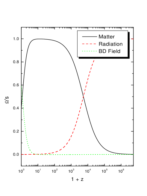
Figure 1: Evolution of the contributions to the critical density for an inverse square potential in a Brans-Dicke theory with $\omega=500$. $H_{0}=75$ km/s/Mpc and $\Omega_{m,0}=0.4$.

In Figure 2 we show, for the same model, the evolution of the ratio between the effective pressure and densities for the Brans-Dicke field. This ratio evolves strongly during the recent matter era, the reason being that $\rho_{\phi}$ actually crosses zero (from negative to positive values). This is in agreement with Figure 1, which shows the current field domination.

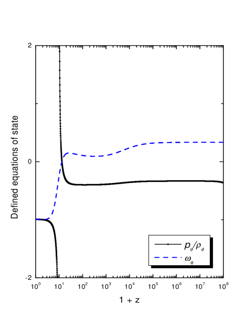
Figure 2: Evolution of the ratio between the effective pressure and densities for the Brans-Dicke field ($p_{\phi}/\rho_{\phi}$), and of the effective equation of state for the field ($w_{\phi}$), entering in the observable quantity $H$. The latter quantity is defined in Section IID. Model parameters are as in Figure 1.

Indeed, we can obtain similar results to those presented here changing the form of the potential to a variety of functional dependencies on the Brans-Dicke field (see Table I). Most interestingly, we see that at the present age of the universe, the effective equation of state for some potentials [we remark here that this is an abuse of language, as will be explained below] is smaller than -1. As we stated, the phenomenon of having $p_{\phi}/\rho_{\phi}<-1$ has been referred to as ‘super-quintessence’ by other authors, whereas the corresponding dark energy has been dubbed ‘phantom energy’ faraoni . Apparently, already the simplest potentials one can imagine can be super-quintessence potentials within Brans-Dicke theory. It is true, however, that the amount of super-quintessence we have found (how large is deviation from -1 towards smaller values) is very small. It is indeed much smaller than what other authors claimed before (see in particular Ref. Sen ). However, we note that, apparently, there is a sign mistake in their Klein-Gordon equation (7), the last term in their rhs should be positive, what can be tested by differentiation or comparison with, for example, Eq. (2.3) of Ref. farese or Eq. (2.6) of 22 This can actually produce a much bigger difference from an equation of state equal to -1 (as we numerically tested), and is probably the origin of the discrepancy.

As we have briefly implied above, $p_{\phi}/\rho_{\phi}<-1$ do not have a especially clear physical meaning. Both, $p_{\phi}$ and $\rho_{\phi}$ are made up of terms coming from the Lagrangian density for the field. But they also contain terms coming from the interaction between the field and gravity (through its non-minimal coupling). The crucial aspect, then, is that the ratio $p_{\phi}/\rho_{\phi}$ does not represent an equation of state, like those of the other components, since an equation of the form $\dot{\rho}_{\phi}+3\dot{a}/a(\rho_{\phi}+p_{\phi})=0$ is not fulfilled. We can actually see from first principles why $\dot{\rho}_{\phi}+3\dot{a}/a(\rho_{\phi}+p_{\phi})\neq 0$ . The field equations of Brans-Dicke theory in a general metric are

$$G_{\mu\nu}=\frac{1}{\phi}\left(T_{\mu\nu}^{matter}+T_{\mu\nu}^{\phi}\right),$$ (31)

where $G_{\mu\nu}$ is the Einstein tensor, $T_{\mu\nu}^{matter}$ is the stress-energy tensor for the matter sector of the theory and

$$T_{\mu\nu}^{\phi}=\frac{w}{\phi}\left(\phi_{,\mu}\phi_{,\nu}-\frac{1}{2}g_{\mu\nu}\phi_{,\alpha}\phi^{,\alpha}\right)+\left(\phi_{,\mu;\nu}-g_{\mu\nu}\Delta\phi\right),$$ (32)

with $\Delta$ being the D^′Alambertian operator. Now, if we multiply the previous equation (31) by $\phi$ and take covariant derivatives, it can be seen that BD

$$T^{\mu\nu\;\;\phi}_{;\nu}=\left(\phi G_{\mu\nu}\right)_{;\nu}$$ (33)

so that, whereas the usual continuity equation for matter is valid, the continuity equation for the above-defined ‘stress-energy tensor’ for the field gets complicated.

IV.4 Observable quantities and the equation of state

Then, if not $p_{\phi}/\rho_{\phi}$, which is the relevant (physically meaningful) quantity to be considered as the equation of state for the field in Brans-Dicke theory? We suggest that the important quantity to look at should come from what we actually measure. In the case of the homogeneous problem we are analyzing, this is the Hubble parameter, $H$. If we rewrite the first of the Friedmann-Robertson-Walker equations as

$$H^{2} = \frac{1}{3}\left(\rho_{fluid}+\tilde{\rho}_{\phi}\right)$$ (34)

$$= \frac{1}{3}\left(\rho_{m,0}a^{-3}+\rho_{r,0}a^{-4}+\tilde{\rho}_{\phi\,0}a^{-3(1+w_{\phi})}\right),$$

then, $w_{\phi}$ is what is going to establish the departure from the predictions of General Relativity plus cosmological constant or a generic quintessence potential of a minimally coupled field. To be specific, if $w_{\phi}=-1$, the theory would be indistinguishable from General Relativity plus cosmological constant (from an observational point of view). If $w_{\phi}>-1$, then the theory would be indistinguishable from a normal (minimally coupled) scalar field with a given potential. And finally, only if $w_{\phi}<-1$, the theory would be observationally different from its general relativistic counterparts: $w_{\phi}<-1$ is a value that cannot be attained by any minimally coupled potential, as we discussed in the Introduction. In that case, super-quintessence adopts its rightful meaning: a super-accelerated expansion of the universe, contrary to the case in which it just represent a particular relationship between quantities importing no physically clear concept. In the previous equation, and to be consistent with the generalized field equations of the theory, we have defined

$$\;\;\tilde{\rho}=\tilde{\rho}_{0}a^{-3(1+w_{\phi})}=-\rho_{m,0}a^{-3}-$$

$$\rho_{r,0}a^{-4}+\frac{1}{\phi}\left(\rho_{m,0}a^{-3}+\rho_{r,0}a^{-4}+\rho_{\phi}\right),$$ (35)

where sub-indices $m,r$ and 0 stand for matter, radiation, and current values, respectively. By definition,

$$w_{\phi}=-1-\frac{1}{3}\ln\left(\frac{\tilde{\rho}_{\phi}}{\tilde{\rho}_{\phi\,0}}\right)\frac{1}{\ln(a)}.$$ (36)

In Figure 2 we have already shown the evolution of this quantity in time (redshift). We also see that, although some non-minimally coupled Brans-Dicke field can effectively produce super-quintessence when supported by particular potentials, the effective ‘equation of state’ being less than -1, its value is too close to -1 so as to effectively mimics a cosmological constant at the current epoch. In Table I we show that the same, almost imperceptible, deviation from an effective cosmological constant appears for other potentials. This is then showing a sign of caution when analyzing the impact of non-minimally coupled theories using the equation of state: differences are actually too small and fall below the threshold of any current or foreseen experiment.

Table 1: Values of the effective and phenomenological ‘equations of state’ for the Brans-Dicke field for different potentials. Model parameters are $\omega=500$, $\Omega_{r}=4.17\times 10^{-5}/h^{2}$, $\Omega_{m}=0.4$, and $H_{0}=75$ km/s/Mpc.

$f(\phi)$	$\left(p_{\phi}/\rho_{\phi}\right)_{today}$	$\left(w_{\phi}\right)_{today}$
$\phi^{-1/2}$	-0.9967	-0.9973
$\phi^{1/2}$	-0.9986	-0.9993
$\phi^{-3/2}$	-0.9947	-0.9953
$\phi^{3/2}$	-1.0006	-1.0013
$\phi^{-1}$	-0.9957	-0.9963
$\phi^{2}$	-1.0016	-1.0023
$\phi^{-2}$	-0.9937	-0.9943
$\phi^{4}$	-1.0056	-1.0063
$\phi^{-4}$	-0.9897	-0.9903
$\phi^{6}$	-1.0096	-1.0103
$\phi^{-6}$	-0.9857	-0.9863
$e^{\phi}$	-0.9997	-1.0003
$e^{-\phi}$	-0.9957	-0.9963
$\cos(\phi)+1$	-0.9966	-0.9972

IV.5 The meaning of $w_{\phi}$

Is $w_{\phi}$ representing an equation of state in the usual sense? In other words, is the equation $\dot{\tilde{\rho}}_{\phi}=-3H(1+w_{\phi})\tilde{\rho}_{\phi}\ ,$ satisfied? To answer this question we shall rewrite the field equations for a general non-minimally coupled theory as per2

$$G_{\mu\nu}=\tilde{T}_{\mu\nu},$$ (37)

where we have defined a new stress-energy momentum tensor, on purpose, to make the previous equation valid:

$$\tilde{T}_{\mu\nu}=T_{\mu\nu}^{fluid}+\tilde{T}_{\mu\nu}[\phi]\ .$$ (38)

As a consequence of the contracted Bianchi identities $\tilde{T}_{\mu\nu}$ is conserved. And since there are no explicit coupling between matter and fields, their corresponding energy-momentum tensors are also separately conserved:

$$\nabla^{\mu}T_{\mu\nu}^{fluid}=\nabla^{\mu}\tilde{T}_{\mu\nu}[\phi]=0\ .$$ (39)

In this framework, reporting no more than a rewriting of the field equations i.e. introducing no new physics at all, the explicit expression for $\tilde{T}_{\mu\nu}[\phi]$ is given by

$$\tilde{T}_{\mu\nu}[\phi]=\omega\left[\nabla_{\mu}\phi\nabla_{\nu}\phi-{1\over 2}g_{\mu\nu}\nabla^{\lambda}\phi\nabla_{\lambda}\phi\right]-$$

$$Vg_{\mu\nu}+\nabla_{\mu}\nabla_{\nu}F-g_{\mu\nu}\Delta F+\left(1-F\right)G_{\mu\nu}\ .$$ (40)

In order to obtain Eq. (37) we have just added and subtracted $G_{\mu\nu}$ on the left hand side of the generalized Einstein equations, i.e.

$$G_{\mu\nu}F=T_{\mu\nu}^{fluid}+T_{\mu\nu}^{field},$$

with the usually defined

$$T_{\mu\nu}^{field}=\omega\left[\nabla_{\mu}\phi\nabla_{\nu}\phi-{1\over 2}g_{\mu\nu}\nabla^{\lambda}\phi\nabla_{\lambda}\phi\right]-$$

$$Vg_{\mu\nu}+\nabla_{\mu}\nabla_{\nu}F-g_{\mu\nu}\Delta F.$$ (41)

This immediately fixes the expression of $\tilde{T}_{\mu\nu}[\phi]$ above. The new effective energy density and pressure that this defined stress-energy density produces are

$$\tilde{\rho}_{\phi}=\omega{{\dot{\phi}}^{2}\over 2}+V(\phi)-3H\dot{F}+3{H^{2}}\left(1-F\right)\ ,$$ (42)

$$\tilde{p}_{\phi}=\omega{\dot{\phi}^{2}\over 2}-V(\phi)+2{H}\dot{F}+\ddot{F}-(3H^{2}+2\dot{H})\left(1-F\right)\ ,$$ (43)

In the case of Brans-Dicke theory, we recall, $\omega=\omega_{BD}/\phi$ and $F=\phi$. Note then that $\tilde{\rho}_{\phi}=\rho_{\phi}+3H^{2}(1-F)$, where $\rho_{\phi}$ was given in Eq. (27). The defined equation of state, $w_{\phi}$, thus, is exactly that given by $\tilde{p}_{\phi}/\tilde{\rho}_{\phi}$, since it was defined using the same Friedmann equation $H^{2}=1/3(\rho_{fluid}+\tilde{\rho}_{\phi})$. Indeed,

$$\tilde{\rho}_{\phi} = -\rho_{fluid}+\frac{1}{F}(\rho_{fluid}+\rho_{\phi})$$ (44)

$$= -\rho_{fluid}+3H^{2}$$

$$= -(3H^{2}F-\rho_{\phi})+3H^{2}$$

$$= \rho_{\phi}+3H^{2}(1-F)$$

At the same time, we can see that

$$\tilde{p}_{\phi}=p_{\phi}-(3H^{2}+2\dot{H})\left(1-F\right).$$ (45)

We conclude that the definition for $w_{\phi}$ represents a real equation of state, since it is supported by a conservation law, and that it is this the one that should be taken into account to compare with the predictions of GR, since it is directly related to the observable, $H$. We can also see, from Table I, that the difference between $w_{\phi}$ and the ratio $p_{\phi}/\rho_{\phi}$ is very small. The reasons that leads to this are explicitly discussed for NMC theories in Section III, a similar argument applies here as well.

IV.6 CMB-related observables

The evolution of the comoving distance from the surface of last scattering (defined as $z=1000$, equivalently $\ln a=-6.90$) can be computed, for different theories, as:

$$\int d\tau=\int_{0.001}^{a}\;\;\frac{da}{a^{2}H(a)}.$$ (46)

Only in the case of extremely low coupling factors (e.g. $\omega$ of Brans-Dicke theory), discarded by current constraints, we see a noticeable difference with the result of General Relativity plus cosmological constant. To give a quantitative idea we can quote the ratio

$$\frac{\tau_{BD}-\tau_{GR}}{\tau_{GR}},$$

calculated today ($a=1$), which, for $\omega=25$ results equal to -0.014, whereas for $\omega=500$ is $-5.7\;10^{-4}$, and quickly tends to zero for bigger values of $\omega$.

The angular scales at which acoustic oscillations occur are directly proportional to the size of the CMB sound horizon at decoupling, that in comoving coordinates is roughly $\tau_{dec}/\sqrt{3}$, and inversely proportional to the comoving distance covered by CMB photons from last scattering until observation, that is $\tau_{0}-\tau_{dec}$ Hu1 . The multipoles scale as the inverse of the corresponding angular scale, and so

$$\ell_{peak}\propto{\tau_{0}-\tau_{dec}\over\tau_{dec}}\ .$$ (47)

As in the non-minimally coupled models studied in Ref. bacci2 , $\tau$ changes because of a different dependence of the Hubble length $H^{-1}$ in the past. However, we have already noted that this change is almost imperceptible when compared with usual General Relativity plus a cosmological constant, unless of course (violating current constraints) the coupling parameter $\omega$ is low enough.

The Integrated Sachs-Wolfe effect makes the CMB coefficients on large scales, small $\ell$’s, change with the variation of the gravitational potential along the CMB photon trajectories Hu . This is undoubtedly changed because of a variation in the gravitational constant since the time of decoupling. However, we expect this change to be also very small, since the $G$-variation we have found, for values of $\omega=500$ and bigger, are typically less than 2% since the time of decoupling.

The scale entering the Hubble horizon at the matter-radiation equivalence is also important, since it will define the matter power turnover Coble . The shift in the power spectrum turnover is given by bacci2

$${\delta k_{turn}\over k_{turn}}=-\left({\delta H^{-1}\over H^{-1}}\right)_{eq}\ ,$$ (48)

and again, this reports a very small difference for all currently possible $\omega$-values. Only for $\omega=25$ this difference is about 12% (where a case of a power law potential with exponent equal to -2 taking as an example). For $\omega=500$ and bigger, the differences are less than 1% (to give a precise example it reports a 0.7% difference in the same power law case as commented before and $\omega=500$). Contrary to what Baccigalupi et al. have done in the past perrota , we are not comparing two different theories (Brans-Dicke and General Relativity) with the same potential, but rather, and motivated by the findings of this section, Brans-Dicke theory with any given potential and General Relativity plus $\Lambda$. It is in this case that the possibilities of actually distinguishing both situations diminish.

V Non-minimally coupled Theories

The details of the cosmological evolution using the general action (III) above, with $\omega=1$ and

$$F(\phi)=1+\xi\phi^{2}$$ (49)

were explored in Refs. perrota ; per2 ; bacci2 , among many others, and we refer the reader to these works and references therein for additional relevant discussions. Our numerical code is in agreement with the results therein reported, and it is a direct extension of the numerical implementation reported in Section IIIB.

In this Section, following the previous discussion, we would like to focus on the possible definitions of equations of state and their impact onto observable quantities. Just as an example, we show in Figure 3 the case of a tracking potential of the form $V=V_{0}\phi^{-2}$, $H_{0}=70$km/s/Mpc, in a flat universe with $\Omega_{m,0}=0.4$. The equivalent Brans-Dicke parameter (obtained by redefining fields in Eq. (III) in order for it to look like a Brans-Dicke theory) is $\omega_{JBD}=\omega F/F_{,\phi}^{2}$, and its value is given by defining $\xi$. The value of $\xi$ used in the model of Figure 3 and successive ones is 5.8 $10^{-3}$, what implies an equivalent Brans-Dicke parameter $\omega_{BD}=3071$, well in agreement with current constraints.

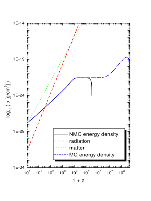
Figure 3: Matter, radiation and quintessence energy densities, both non-minimally (NMC) and minimally coupled (MC). The incomplete curve corresponds to the non-minimally coupled quintessence, and the cutoff is produced by a change in the sign of the effective density, see text for details.

Starting from the general field equations, we can immediately define, as done for the Brans-Dicke theory, an effective energy density and pressure for the scalar field. The former, for instance, appears writing the 00-component of the field equation as $H^{2}=1/{3F}\left(\rho_{fluid}+\rho_{\phi}\right).$ The explicit expression then being,

$$\rho_{\phi}={\omega\over 2}\dot{\phi}^{2}+V-3{H}\dot{F}$$ (50)

for the energy density, and

$$p_{\phi}=\frac{\omega}{2}\dot{\phi}^{2}-V+2H\dot{F}+\ddot{F}$$ (51)

for the pressure. These two expressions do not, as we have shown before, pertain to a conserved energy-momentum tensor. They do, however, define an effective equation of state, this being just $p_{\phi}/\rho_{\phi}$. This relationship is subject to same caveats mentioned above for the case of Brans-Dicke: it is neither positive nor negative defined, since the effective energy density itself shifts its sign during the evolution. The energy density quoted above is what is depicted (whenever possible) in Figure 3. As it can be seen, it tracks closely the usually defined minimally coupled (MC) energy density at low redshifts, this being an effect of the necessarily small coupling $\xi$ that is adopted to fulfill observational constraints.

Again, in order to work with a conserved energy-momentum tensor, we can rewrite the field equations and obtain a real equation of state, $w_{\phi}=\tilde{p}_{\phi}/\tilde{\rho}_{\phi}$, where $\tilde{\rho}_{\phi}$ and $\tilde{p}_{\phi}$ were given in Eqs. (42) and (43), respectively. As we already mentioned in the case of Brans-Dicke, this equation of state is exactly what results in writing the field equation as $H^{2}=1/3(\rho_{fluid}+\varrho_{\phi})$, defining implicitly $\varrho_{\phi}=1/F(\rho_{fluid}+\rho_{\phi})-\rho_{fluid}.$ Finally, just for comparison, one can as well consider the equation of state for the case of a minimally coupled scalar field, $p/\rho$, with

$$\rho={1\over 2}\dot{\phi}^{2}+V(\phi)\ ,$$ (52)

$$p={1\over 2}\dot{\phi}^{2}-V(\phi)\ .$$ (53)

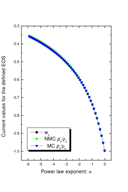
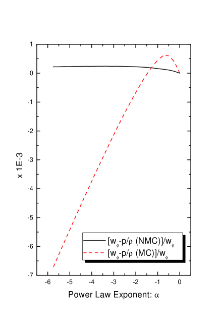
Figure 4: Left: Current values of the defined ’equations of state’, see text, as a function of the power law exponent of the tracking potential. Right: Difference between the equation of state directly related with the Hubble parameter, $w_{\phi}$ and the non-minimally coupled (NMC) and minimally coupled $p_{\phi}/\rho_{\phi}$.

In Figure 4 we show the results of these different definitions of equation of state for the current time, as a function of the exponent of the power law potential $V=V_{0}\,\phi^{\alpha}$, for a flat universe model given by $\Omega_{m,0}=0.4$, the same model used in Figure 3. We see that they do not present noticeable differences. Very low values of the power law exponent (shallow potentials) are needed to produce equations of state near that generated by a cosmological constant. To be quantitative, Figure 4 also shows, in the right panel, the differences between the equation of state directly related with the Hubble parameter, $w_{\phi}$ and the non-minimally coupled (NMC) and minimally coupled $p_{\phi}/\rho_{\phi}$. Clearly, the differences are minor. One can actually understand why these differences are so small. Note that the energy density and pressure in a non-minimally coupled field theory can be written as the minimally coupled ones plus additional terms. In the case of $\tilde{\rho}_{\phi}$, these terms are equal to $-3H\dot{F}+3H^{2}(1-F)$, whereas for $\rho_{\phi}$ only the first term above enters. Both these terms are, however, proportional to $\xi$, being themselves

$$-3H\dot{F}+3H^{2}(1-F)\sim-6\xi H\dot{\phi}-3\xi H^{2}\phi^{2}.$$

But since from the evolution of the field, ${\cal O}(H^{-1}\dot{\phi})$=1 today, and at the current era, ${\cal O}(H^{2})\sim V$, the energy density can be written as $\tilde{\rho}_{\phi}\sim\rho_{mc}-3\xi(\frac{\dot{\phi}^{2}}{2}+V\phi^{2})$, where $\rho_{mc}$ is the minimally coupled energy density. Clearly, at the current cosmological era and because of the constraints on $\xi$, the second terms are sub-dominant in comparison to the first ones. A similar analysis can be established for the pressure, where again all extra terms are proportional to $\xi$, and then for the equations of state. Today the influence of the last terms in Eqs. (42) and (43), the ‘gravitational dragging’ terms, as dubbed in Ref. per2 , is negligible in comparison to the minimally coupled contribution. It is only in the past, when the matter density dominates the evolution of the universe, that these terms become important.

The previous analysis is not valid in the past history of the universe. Figure 5 shows the evolution of the different equations of state with redshift. We can see that the scaling solution of the tracking potentials (equation of state is approximately equal to $-2/(2+\alpha)$ between $z\sim$1–1000, when $\rho_{matter}>\rho_{\phi}$, see for e.g. Refs. perrota ; per2 ), appears for all defined equations of state but $w_{\phi}$. We also note that because of the sign non-definiteness of the defined non-minimally coupled effective ‘energy density’, the corresponding equation of state shows sudden changes at high redshift, in the position where the density cross zero. Finally, we find that for tracking non-minimally coupled quintessence, there is no super-quintessence potential in any of the defined equations of state, not even by an small amount, all of them being greater than -1 at present. This latter result is actually valid for all potentials analyzed (similar cases than those presented in Table I).

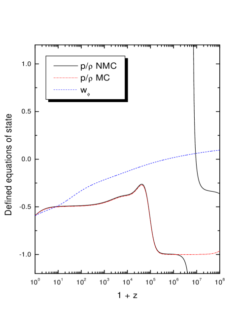
Figure 5: Evolution in redshift of the equations of state for a model with $V\propto\phi^{-2}$.

V.1 Comments on perturbations and on the possible degeneracy with kinetically driven quintessence

Perturbations analysis of the field equations, as done by Perrotta and Baccigalupi per2 , have shown that rich phenomena are uncovered when working with the field equations written as in (37). The most important of them are those generated by gravitational dragging, exclusive of non-minimally coupled theories. This phenomenon is, basically, the early dominance of the last term in Eqs. (42) and (43), which is, in turn, produced due to the fact that they are proportional to the square of the Hubble parameter, and then to the total energy density. The latter scales as $a^{-3}$ and $a^{-4}$ at early times, and then makes the gravitational generated term to dominate the dynamics of the field.

The advantage of writing the formalism as in Eq. (37) is the fact that usual perturbation analysis –as applied for any fluid component of the universe– is also valid for the field. In that sense, concepts as the equation of state, or the adiabatic sound speed

$$c^{2}_{\phi}=\frac{\dot{\tilde{p}}_{\phi}}{\dot{\tilde{\rho}}_{\phi}}=w_{\phi}-\frac{1}{3{H}}\frac{\dot{w}_{\phi}}{1+w_{\phi}},$$ (54)

(where we have made use of the field conservation equation) can be well defined. If the field is slowly varying in time, $c^{2}_{\phi}\sim w_{\phi}$. Hu Hu showed, for negative equations of state, that adiabatic fluctuations are unable to give support against gravitational collapse. Density perturbations would become non-linear after entering the horizon, unless the entropic term $w_{\phi}\Gamma_{\phi}>0$ Hu .

The effective sound speed, $c_{{{\rm eff}}\,,\phi}^{2}$, is then defined in the rest frame of the scalar field, where $\delta T^{0}_{j\,\phi}=0$ Hu . The gauge invariant entropic term is written as $w_{\phi}\Gamma_{\phi}=(c_{{\rm eff}}^{2}-c_{\phi}^{2})\delta_{\phi}^{(rest)}\ ,$ where $\delta_{\phi}^{(rest)}$ is the density contrast in the dark energy rest frame per2 $\delta_{\phi}^{(rest)}=\delta_{\phi}+3{{\cal{H}}\over k}\left(1+w_{\phi}\right)\left(v_{\phi}-B\right)$ (we refer the reader to Ref. per2 for more careful explanations). For normal quintessence, the effective sound speed is $c_{{{\rm eff}}\,,\phi}^{2}=1$, giving a relativistic behavior to the corresponding density fluctuations. However, Perrotta and Baccigalupi per2 have found that the situation can be much different for non-minimally coupled gravity. In that case,

$$c_{{{\rm eff}}\,,\phi}^{2}\sim{\delta\tilde{p}_{\phi}\over\delta\tilde{\rho}_{\phi}}$$ (55)

for values of $k\gg{H}$. But because of gravitational dragging, $\delta\tilde{\rho}_{\phi}$ can be quite difference from the usual case, and this ratio may be much lower than unity whenever the energy density perturbations of the scalar field are enhanced by perturbations in the matter field. At the level of perturbations, then, quite distinctive effects appears in non-minimally coupled quintessence as compared with the usual case and make these theories possibly distinguishable.

Very recently, yet another scenario for an alternative model of quintessence was introduced picon . In it, known as $k$-essence, the Lagrangian density includes a non-canonic kinetic term:

$$S=\int d^{4}x\sqrt{-g}\left({1\over 16\pi G}R+p(\phi,\nabla\phi)\right)+S_{m,r},$$ (56)

where $S_{m,r}$ denotes the action for matter and/or radiation. Examples in which the Lagrangian depends only on the scalar field $\phi$ and its derivative squared $X=-{1\over 2}\nabla^{\mu}\phi\nabla_{\mu}\phi.$ have been constructed picon . The field equations for this models are

$$R_{\mu\nu}-{1\over 2}g_{\mu\nu}R=\;\;\;\;\;\;\;\;\;\;\;\;\;\;\;\;\;\;\;\;\;\;\;\;\;\;\;\;\;\;\;\;\;\;\;\;\;$$

$$8\pi G\left(\frac{\partial p(\phi,X)}{\partial X}\nabla_{\mu}\phi\nabla_{\nu}\phi+p(\phi,X)g_{\mu\nu}+T^{m,r}_{\mu\nu}\right)$$ (57)

where $T^{m,r}_{\mu\nu}$ is the energy-momentum tensor for usual matter fields. $p(\phi,X)$ corresponds to the pressure of the scalar field, whereas the energy density is given by $\rho_{\phi}=2X\partial p/\partial X-p$ picon2 . It can be seen that for this models, the speed of sound is given by erik

$$c_{{\rm eff}}^{2}={p_{Q,X}\over\rho_{Q,X}}={p_{,X}\over p_{,X}+2Xp_{,XX}}.$$ (58)

Apparently, then, and since $p$ is completely generic, it could exist a non-canonic kinetic term within $k$-essence giving rise to the same results of non-minimally coupled gravity. Viscosity (a parameter relating velocity and metric shear with anisotropic stress Hu ) can however provide the way to break the degeneracy, since it results non-zero for a non-minimally coupled field (contrary as well to what results in usual quintessence) per2 .

VI Conclusions

In the case of Brans-Dicke theory, and in the cases of $\omega_{BD}$ allowed by current constraints, we have numerically proven that the homogeneous field equations of extended quintessence yield to no observable effect that can distinguish the theory from the predictions of General Relativity plus a cosmological constant. It is with this model that the comparison should be made, since for the large values of the coupling parameters required by current experiments, all potentials are closely similar to a constant function, and the theory itself to General Relativity. Although we have not made a detailed perturbation analysis using the full numerical CMBFAST code, we can safely predict that the same situation will happen there, as a result of the analysis made for the CMB-related observables in Section IIC. We discussed the observationally-related definition of equation of state $w_{\phi}$, and not to the usually studied ratio between the effective pressure and density directly obtained from the field equations, to which we assign no particular physical meaning. The phenomenon of super-quintessence, i.e. a super-accelerated expansion of the universe, although possible for a non-minimally coupled Brans-Dicke scalar field, and impossible in any minimally coupled field situation, it is of such an small amount that is far beyond the expectations of any realistic experiment. From a practical point of view, then, it will always exist a scalar field potential supporting a minimally coupled field that produces experimentally indistinguishable results from those obtained within the extended quintessence framework of Brans-Dicke theory.

For the more general extended non-minimally coupled models studied, the possibility of having super-quintessence actually disappears: all tracking potentials explored produce effective equations of state greater than -1. We have shown that for low values of the exponent in the tracking potentials supporting the non-minimally coupled field (i.e. equations of state are close to -1), the difference among all defined equations of state is negligible. It is, however, in the perturbation regime where differences with the usual quintessence case can be noticed. As Perrotta and Baccigalupi have found per2 , a new gravitational dragging effect appears here, giving rise to the possibility of clumps of scalar field matter. In this case, however, it is with $k$-essence models that a degeneracy could appear, particularly in those cases in which $p_{,X}+2Xp_{,XX}\gg 1$, yielding the speed of sound to values close to zero.

Finally, we remark that expanding solutions where acceleration is transient have been recently considered given the consistency problem between string theory and spaces with future horizons hellerman . Since scalar-tensor theories of gravity likely originate in string theory, it would be interesting to make a similar analysis to that presented in the previous reference for the case of non-minimally coupled theories.

Appendix

In the literature, one may find two alternative introductions of general non-minimally coupled theories. Firstly, the one that we follow in Section II (see for instance PRL ), and secondly, the one that is derived from the action

$$S=\int d^{4}x\sqrt{-g}\left[{1\over 2\kappa}f(\phi,R)-{\omega(\phi)\over 2}\nabla^{\mu}\phi\nabla_{\mu}\phi\right.$$

$$\left.-V(\phi)+L_{fluid}\right]\ ,$$ (59)

where $\kappa$ is a constant, not necessarily taken as 1, and plays the role of the “bare” gravitational constant (see for instance farese , by the same authors). The function $f$ is then assumed to be of the form

$$(1/\kappa)f(\phi,R)=F(\phi)\,R.$$ (60)

The function $F$, in the case we are interested in, is written as

$$F(\phi)=\frac{1}{\kappa}+\xi\phi^{2}=1+\xi(\phi^{2}-\phi_{0}^{2}).$$ (61)

Then, a value of $\kappa=1$, as we have taken in the theoretical development of the previous sections just reduces to take $\phi_{0}$, the current value of the field, equal to 0. This, however, is not what may result, in general, numerically convenient, since it would imply to precisely fix the evolution of the field to reach $\phi=0$ today. Instead, as we are not actually interested in any value of $\kappa$ per se, we do not make $\kappa=1$ in our numerical code, and instead follow the treatment given by Perrotta and Baccigalupi (per2 ). In that case, they choose to rewrite the field equations as

$$G_{\mu\nu}=\kappa T_{\mu\nu},$$ (62)

with the corresponding field energy density and pressure given by

$$\tilde{\rho}_{\phi}=\omega{{\dot{\phi}}^{2}\over 2}+V(\phi)-3H\dot{F}+3{H^{2}}\left(\frac{1}{\kappa}-F\right)\ ,$$ (63)

$$\tilde{p}_{\phi}=\omega{\dot{\phi}^{2}\over 2}-V(\phi)+2{H}\dot{F}+\ddot{F}-(3H^{2}+2\dot{H})\left(\frac{1}{\kappa}-F\right)\ .$$ (64)

When comparing Eq. (62) with the usual Einstein equations, one has to take into account that the value of $\kappa$ is not 1 (although certainly it is truly close to unity, because of the constraint imposed on $\xi$). Then, if we decide to write the Friedman equation like $H^{2}=1/3(\rho_{fluid}+\varrho_{\phi})$, to directly compare with GR (and the same matter density) the corresponding relationship between $\varrho_{\phi}$ and $\tilde{\rho}_{\phi}$ give in Eq. (63) is

$$\varrho_{\phi}=(\kappa-1)\rho_{fluid}+\kappa\tilde{\rho}_{\phi}.$$ (65)

In this scheme, $\tilde{p}_{\phi}/\tilde{\rho}_{\phi}$ (with quantities defined as in Eqs. (63) and (64)) will differ from the equation

$$w_{\phi}=-1-\frac{1}{3}\ln\left(\frac{\varrho_{\phi}}{\varrho_{\phi\,0}}\right)\frac{1}{\ln(a)},$$ (66)

because $\varrho_{\phi}\neq\tilde{\rho}_{\phi}$, but it is the latter Eq. (66) what should be used to compare with the results of General Relativity with a fixed current matter density.

References

- (1) A. Riess et al. Astron. J 116, 1009 (1998); S Perlmutter et al. ApJ 517 565 (1999).
- (2) See, for example, P. De Bernardis et al., ApJ, 564, 559 (2002).
- (3) P. J. Peebles, B. Ratra, Astrophys. J. 352, L17 (1988); R.R. Caldwell, R. Dave, P. J. Steinhardt, Phys. Rev. Lett. 80, 1582 (1998).
- (4) V. Sahni, and A. Starobinsky, Int.J.Mod.Phys. D9,373 (2000).
- (5) L. Wang, R. R. Caldwell, J. P. Ostriker, P. J. Steinhardt, ApJ 530, 17 (2000); P.J. Steinhardt, L. Wang, I. Zlatev, Phys. Rev. D59, 123504 (1999); I. Zlatev, L. Wang, P.J. Steinhardt, Phys. Rev. Lett. 82, 896 (1999); A.R. Liddle, R.J. Scherrer, Phys. Rev. D59, 023509 (1999).
- (6) V. Faraoni, astro-ph/0110067 (2001); E. Gunzig, A. Saa, L. Brenig, V. Faraoni, T.M. Rocha Filho and A. Figueiredo, Phys. Rev. D63 067301, (2001).
- (7) R. R. Caldwell, astro-ph/9908168
- (8) S. Sen and T. R. Seshadri, To be published in Int. J. Mod. Phys. D, gr-qc/0007079
- (9) F. Perrotta, C. Baccigalupi, and S. Matarrese, Phys. Rev. D61, 023507 (1999).
- (10) F. Perrotta, and C. Baccigalupi, astro-ph/0201335
- (11) J. P. Uzan, Phys.Rev. D59, 123510 (1999); A. Riazuelo and J. P. Uzan, astro-ph/0107386
- (12) G. Espósito-Farese, and D. Polarski, Phys. Rev. D63, 063504 (2001).
- (13) T. Chiba, Phys. Rev. D64, 103503 (2001).
- (14) L. Amendola, Phys. Rev. D60, 043501 (1999); O. Bertolami and P. Martins, Phys. Rev. D61, 064007 (2000); D. Holden and D. Wands, Phys. Rev. D61, 043506 (2000); Y. Fujii, Phys. Rev. D62, 044011 (2000); F. Perrotta and C. Baccigalupi astro-ph/0205245; S. Capozziello, Int. J. Mod. Phys. D11, 483 (2002).
- (15) C. Santos, and R. Gregory, Annals Phys. 258, 111 (1997).
- (16) M. Visser, Lorentzian Wormholes (AIP, New York, 1996).
- (17) C. Barceló and M. Visser, Phys. Lett. B466, 127 (1999); C. Barcelo and M. Visser, Class. Quant. Grav. 17, 3843 (2000).
- (18) J. Cramer, R. Forward, M. Morris, M. Visser, G. Benford, and G. Landis, Phys. Rev. D 51, 3117 (1995); D. F. Torres, E. F. Eiroa and G. E. Romero, Mod. Phys. Lett. A 16, 1849 (2001); M. Safonova, D. F. Torres and G. E. Romero, Phys. Rev. D 65, 023001 (2002); E. Eiroa, G. E. Romero and D. F. Torres, Mod. Phys. Lett. A 16, 973 (2001); M. Safonova, D. F. Torres and G. E. Romero, Mod. Phys. Lett. A 16, 153 (2001); L. A. Anchordoqui, S. Capozziello, G. Lambiase and D. F. Torres, Mod. Phys. Lett. A 15, 2219 (2000); L. A. Anchordoqui, G. E. Romero, D. F. Torres and I. Andruchow, Mod. Phys. Lett. A 14, 791 (1999); G. E. Romero, D. F. Torres, I. Andruchow, L. A. Anchordoqui and B. Link, Mon. Not. Roy. Astron. Soc. 308, 799 (1999); D. F. Torres, G. E. Romero and L. A. Anchordoqui, Mod. Phys. Lett. A 13, 1575 (1998); ibid. Phys. Rev. D 58, 123001 (1998).
- (19) A. DeBenedictis and A. Das [gr-qc/0009072]; S. E. Perez Bergliaffa and K. E. Hibberd, Phys. Rev. D 62, 044045 (2000); C. Barcelo and M. Visser, Nucl. Phys. B584, 415 (2000); L. A. Anchordoqui and S. E. Perez Bergliaffa, Phys. Rev. D 62, 067502 (2000); D. Hochberg, A. Popov, and S. V. Sushkov, Phys. Rev. Lett. 78, 2050 (1997); S. Kim and H. Lee, Phys. Lett. B 458, 245 (1999); S. Krasnikov, Phys. Rev. D 62, 084028 (2000); D. Hochberg and M. Visser, Phys. Rev. D 56, 4745 (1997); L. A. Anchordoqui, S. Perez Bergliaffa and D. F. Torres, Phys. Rev. D 55, 5226 (1997); L. A. Anchordoqui, D. F. Torres, M. L. Trobo and S. E. Perez Bergliaffa, Phys. Rev. D 57, 829 (1998).
- (20) M. Visser, Phys. Rev. D 56, 7578 (1997); Science 276, 88 (1997).
- (21) A. R. Liddle and D. H. Lyth, Cosmological inflation and large scale structure, (Cambridge University Press, Cambridge, 2000, pp. 20).
- (22) R. D. Reasenberg et al., Astrophys.J. 234, L219 (1979).
- (23) See C. Will, gr-qc/0103036
- (24) C. M. Will, Theory and Experiment in Gravitational Physics, (Cambridge University Press, Cambridge, England, 1993).
- (25) B. M. Barker, ApJ 219, 5 (1978).
- (26) F. S. Accetta, L. M. Krauss and P. Romanelli, Phys. Lett. B248, 146 (1990); D. F. Torres, Phys. Lett. B 359, 249 (1995); J. A. Casas, J. García-Bellido and M. Quirós, Mod. Phys. Lett. A7, 447 (1992), Phys. Lett. B278, 94 (1992); D. I. Santiago, D. Kalligas, R. V. Wagoner, Phys. Rev. D56, 7627 (1997); A. Serna, R. Domingues-Tenreiro and G. Yepes, ApJ 391, 433 (1992).
- (27) J. P. Mimoso, and D. Wands, Phys. Rev. D52, 5612 (1995).
- (28) J. D. Barrow, and J. P. Mimoso, Phys. Rev. D50, 3746 (1994); J. D. Barrow, and P. Parsons, Phys. Rev. D55, 1906 (1997).
- (29) D. F. Torres and H. Vucetich, Phys. Rev. D 54, 7373 (1996); D. F. Torres, Phys. Lett. A 225, 13 (1997).
- (30) C. Brans and R. H. Dicke, Phys. Rev. 124, 925 (1961).
- (31) A. R. Liddle, A. Mazumdar, and J. D. Barrow, Phys. Rev. D58, 027302 (1998).
- (32) D. I. Santiago, and A. S. Silbergleit Gen. Rel. Grav. 32, 565 (2000).
- (33) S. Weinberg, Gravitation and cosmology (Wiley, New York, 1972).
- (34) W. Hu, U. Seljak, M. White, M. Zaldarriaga, Phys. Rev. D57, 3290 (1998).
- (35) K. Coble, S. Dodelson, and J. Friemann, Phys. Rev. D55, 1851 (1997).
- (36) C. Baccigalupi, S. Matarrese, and F. Perrotta, Phys. Rev. D62, 123510 (1999).
- (37) T. Chiba, T. Okabe, and M. Yamaguchi, Phys. Rev. Phys. Rev. D62, 023511 (2000), C. Armendariz-Picon, V. Mukhanov, and P. J. Steinhardt, Phys. Rev. Lett. 85, 4438 (2000), ibid. Phys. Rev. D63, 103510 (2000).
- (38) C. Armendariz-Picon, T. Damour, and V. Mukhanov, Phys. Lett. B458, 209 (1999).
- (39) W. Hu, ApJ 506, 485 (1998).
- (40) J. K. Erickson, R. R. Caldwell, Paul J. Steinhardt, C. Armendariz-Picon, and V. Mukhanov, astro-ph/0112438
- (41) N. Banerjee and S. Sen, Phys. Rev. D56, 1334 (1997).
- (42) B. Boisseau, G. Espósito-Farese, D. Polarski, and A. A. Starobinsky, Phys. Rev. Lett. 85, 2236 (2000).
- (43) S. Hellerman, N. Kaloper, L. Susskind, JHEP 0106, 003 (2001).