The Amplitude Evolution and Harmonic Content of Millisecond Oscillations in Thermonuclear X-ray Bursts

Abstract

We present a comprehensive observational and theoretical analysis of the amplitudes and profiles of oscillations that occur during thermonuclear X-ray bursts from weakly-magnetized neutron stars in low mass X-ray binaries. Our sample contains 59 oscillations from six sources observed with the Rossi X-ray Timing Explorer. The oscillations that we examined occurred primarily during the decaying portions of bursts, and lasted for several seconds each. We find that the oscillations are as large as 15% during the declines of the bursts, and they appear and disappear because of to intrinsic variations in their fractional amplitudes. However, the maxima in the amplitudes are not related to the underlying flux in the burst. We derive folded profiles for each oscillation train to study the pulse morphologies. The mean rms amplitudes of the oscillations are 5%, although the eclipsing source MXB 1659$-$298 routinely produces 10% oscillations in weak bursts. We also produce combined profiles from all of the oscillations from each source. Using these pulse profiles, we place upper limits on the fractional amplitudes of harmonic and half-frequency signals of 0.3% and 0.6%, respectively (95% confidence). These correspond to less than 5% of the strongest signal at integer harmonics, and less than 10% of the main signal at half-integer harmonics. We then compare the pulse morphologies to theoretical profiles from models with one or two antipodal bright regions on the surface of a rotating neutron star. We find that if one bright region is present on the star, it must either lie near the rotational pole or cover nearly half the neutron star in order to be consistent with the observed lack of harmonic signals. If an antipodal pattern is present, the hot regions must form very near the rotational equator. We discuss how these geometric constraints challenge current models for the production of surface brightness variations during the cooling phases of X-ray bursts.

1 Introduction

Flux oscillations with millisecond periods have been observed during thermonuclear bursts from weakly-magnetized neutron stars in nine different low-mass X-ray binaries (LMXBs; see Strohmayer 2001 for a review). The bursts occur when helium in the accreted material on the stellar surface begins to burn in an unstable regime (see Lewin, van Paradijs, & Taam for a review). Therefore, it has long been expected that anisotropies in the burning could produce pulsations at the stellar spin frequency (e.g. Schoelkopf & Kelley, 1991; Bildsten, 1995; Strohmayer et al., 1996). The amplitudes of the oscillations vary between $1-50\%$ rms, with the largest fractional amplitudes observed in the rises of bursts when there is spectral evidence for growing burning regions (Strohmayer, Zhang, & Swank 1997). Oscillations are observed for up to 15 seconds. Their frequencies evolve by as much as 1.3% during the course of a burst, usually increasing rapidly at first, but appearing to saturate at an asymptotic frequency before they disappear (Strohmayer et al., 1997a). If we account for this frequency evolution, 70% of the oscillations appear coherent (Muno et al., 2002), and the asymptotic frequencies are stable to a few parts in a thousand in bursts separated by several years (Strohmayer & Markwardt, 1999; Muno et al., 2000; Giles et al., 2002). Although the underlying clock may not be perfectly stable, it is nonetheless remarkably good (Muno et al., 2002; Strohmayer & Markwardt, 2002). This strongly suggests that the oscillations are produced by patterns in the surface brightness of these rotating neutron stars.

Several mechanisms have been proposed to explain the frequency evolution of the burst oscillations. Strohmayer et al. (1997a) suggested that the oscillations originate from hot regions on a burning layer that expands and decouples from the neutron star when the nuclear burning commences. The oscillations are observed when the burning layer begins to cool and contract, causing them to increase in frequency as the layer re-couples to the neutron star. However, calculations suggest that a rigidly rotating, hydrostatically expanding burning layer produces too small a frequency drift (see Cumming & Bildsten, 2000; Cumming et al., 2002). Recently, Spitkovsky, Levin, & Ushomirsky (2002) pointed out that vortices could form in a geostrophic flow moving against the rotation of the neutron star, driven by the combination of the Coriolis force and a pressure gradient between the equator and the poles. Like their counterparts on Earth and on Jupiter, such vortices could conceivably appear as light or dark regions on the neutron star. The frequency drift in this model is attributed to the slowing of the geostrophic flow as the burning layer cools. Finally, Heyl (2002) has proposed that global oscillation modes could propagate as waves on the neutron star ocean. The velocity with which these modes travel is extremely sensitive to the vertical density and temperature structure, as well as to the surface composition, and could thus change during the burst. Indeed, in all these models, the mechanisms producing the pulsations depend strongly on the properties of the neutron stars, and the oscillations offer a powerful probe of the physical conditions in their outer layers. In particular, the pulsations may reveal the stellar spin frequency and surface gravity.

All of the above models assume that the oscillations occur near the rotational frequency of the neutron star ($\nu_{\rm spin}$). If this is the case, then the burst oscillations trace the history of accretion torques on the neutron stars in these LMXBs, which are thought to be the progenitors of recycled millisecond radio pulsars (Alpar et al., 1982; Radhakrishnan & Srinivasan, 1982). The frequencies of the oscillations ($\nu_{\rm burst}$) are distributed evenly between 270–620 Hz (Muno et al., 2001). However, there are observational and theoretical reasons to suspect that the subset of the oscillations with $\nu_{\rm burst}\approx 500-600$ Hz occur at twice the spin frequency, corresponding to two antipodal bright regions on the neutron star (Strohmayer et al. 1996; Miller, Lamb, & Psaltis 1998; Miller 1999; van der Klis 2000). Determining whether $\nu_{\rm burst}=2\times\nu_{\rm spin}$ in the subset of sources with 600 Hz oscillations is particularly important, because if $\nu_{\rm spin}\approx 300$ Hz in all nine of these LMXBs, then some mechanism may be limiting the maximum spin frequencies of the neutron stars (e.g., White & Zhang, 1997; Bildsten, 1998).

The propagation of photons from the surface of a rapidly rotating neutron star is affected by general relativity, time delays, and Doppler shifts, and hence these oscillations carry signatures of the physical parameters of the neutron star to an observer (Miller & Lamb 1998; Braje, Romani & Rauch 2000; Weinberg, Miller, & Lamb 2001; Nath, Strohmayer, & Swank 2002). In particular, strong gravitational lensing by the neutron star allows a bright region on its surface to be seen for a large fraction of the rotational period. This, in general, suppresses the amplitudes and reduces the harmonic content of any resulting oscillations (see Weinberg et al., 2001; Özel, 2002). On the other hand, Doppler and time delay effects cause the pulse profiles to be more asymmetric and narrowly-peaked, which increases the amplitudes and the harmonic content of the oscillations (Weinberg et al., 2001; Braje et al., 2000). Thus, the properties of the burst oscillations can constrain the emission geometry and the compactness of the neutron star.

In this paper, we present a comprehensive observational and theoretical investigation of the amplitudes and profiles of burst oscillations, seeking to constrain the geometry of the emission. We focus on oscillations observed during the peak and decline of X-ray bursts with the Rossi X-ray Timing Explorer RXTE. These signals are present for tens of seconds, and thus provide excellent statistics to constrain the pulse profiles and amplitudes of the pulsations (see Nath et al., 2002).

In Section 2, we examine the amplitude evolution and the profiles of the oscillations. In Section 3, we present theoretical predictions of the signal that an observer would see from one or two bright regions on the surface of a rapidly rotating neutron star. We explore a range of parameters relevant to the burst oscillations, and explicitly take into account the response of the RXTE detectors to allow a direct comparison with the data (compare Miller & Lamb, 1998; Braje et al., 2000; Weinberg et al., 2001). In Section 4, we place constraints on the location and size of bright regions on the neutron star surface by comparing the theoretical calculations to observations. Finally, we discuss the implications of these constraints for the various models proposed to explain the burst oscillations.

2 Observations

Our analysis used observations with the Proportional Counter Array (PCA; Jahoda et al. 1996) on RXTE. The PCA consists of five identical gas-filled proportional counter units with a total effective area of 6000 cm² and sensitivity in the 2.5–60 keV range. The detector is capable of recording photons with microsecond time resolution and 256-channel energy resolution. The data were recorded in a wide variety of data modes with different time and energy resolutions, depending upon the details of the original proposed programs and the available telemetry bandwidth. For all of the analysis presented here, we converted the photon arrival times at the spacecraft to Barycentric Dynamical Time (TDB) at the solar system barycenter, using the Jet Propulsion Laboratory DE-200 solar system ephemeris (Standish et al. 1992).

We searched the entire RXTE public data archive for X-ray bursts from 8 neutron stars that are known to exhibit burst oscillations (see Table 1 and Muno et al. 2001). As of September 2001, we have identified a total of 159 X-ray bursts from these 8 sources. Each of these bursts was then searched for millisecond oscillations as described in Muno et al. (2002). Out of the 68 pulse trains detected, 59 persisted continuously for $>2$ s and therefore warranted a more detailed analysis (Table 1). The majority of these continuous pulse trains were observed during the declining portions of the bursts. Although 39 of the 68 oscillation trains were detected during the rises of bursts, only 17 lasted continuously through to the tails. Six oscillations appeared only in the rises of bursts and persisted for less than 1 s, precluding further analysis. The remaining 16 oscillations were observed during the rises and tails of bursts, but disappeared during the peaks. We were only able to analyze these in the tails of the bursts when they re-appeared.

To examine the amplitudes and profiles of the oscillations, we used data containing a single energy channel (2.5–60 keV) and $2^{-13}$ s (122 $\mu$s) time resolution. We modeled the frequency evolution of the oscillations via a phase connection method commonly used in pulsar studies (Manchester & Taylor, 1977). In this technique, we fold the data in short intervals (0.25–0.5 s) about a trial phase model, which is then refined through a least squares fit to the residuals. This provides excellent frequency resolution,

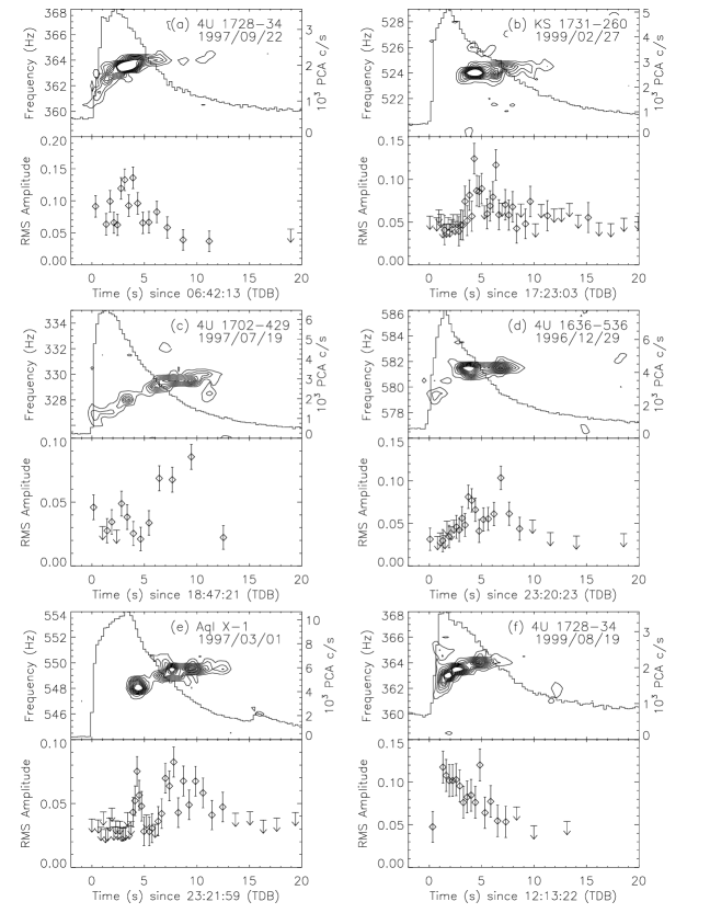
Figure 1: Six examples of oscillations during X-ray bursts. Top Panels: Contours represent the Fourier power as a function of time and frequency, computed from the power spectra of 2 s intervals of data every 0.25 s throughout the burst. A Welch function was used to taper the data to reduce sidebands in the power spectrum due to its finite length (Press et al., 1992). The contour levels are at powers of $0.02$ in single-trial probability starting at a chance occurrence of $0.02$. The PCA count rate (2–60 keV) is also plotted, referenced to the right axis. Bottom Panels: The fractional rms amplitude of the oscillations as a function of time during the burst. The data were folded in intervals that contained a constant count rate, such that each interval is sensitive to oscillations of a constant fractional amplitude (between 4–10%). The amplitudes of the oscillations do not appear to be correlated with the amount of flux from the underlying burst.

and a statistical measure of how well the model reproduces the data (see Muno et al., 2002, for a further description). We folded the 59 continuous oscillation trains about the best-fit frequency models of Muno et al. (2002).

We measured the amplitudes of the oscillations and their harmonics by computing a Fourier power spectrum of the folded profiles. If we normalize the power according to Leahy et al. (1983), the fractional rms amplitude at any multiple of the oscillation frequency is

$$A_{n}=\left({{P_{n}}\over{I_{\gamma}}}\right)^{1/2}{{I_{\gamma}}\over{I_{\gamma}-B_{\gamma}}},$$ (1)

where $P_{n}$ is the power at the $n$th bin of the Fourier spectrum, $I_{\gamma}$ is the total number of counts in the profile, and $B_{\gamma}$ is the estimated number of background counts in the profile. This equation is valid so long as the phase and frequency of the oscillation is known, as it is by design for our folded profiles. Uncertainties and upper limits on the amplitudes are computed taking into account the distribution of powers from Poisson noise in the spectrum, using the algorithm in the Appendix of Vaughan et al. (1994).

The models used were low-order polynomials or exponential functions that reproduced the phase evolution well in 70% of the oscillations. In the remainder of the oscillation trains, there was evidence both for discrete phase jumps and for phase evolution that was only piecewise smooth. Additional power in principle could be recovered from these oscillations with more complicated frequency models, but we believe that the advantage would be small. For instance, we compared the powers we detected at the fundamental frequency to those obtained by Strohmayer & Markwardt (1999) for two oscillations that are common to both samples (bursts on 1997 July 26 and 30 from 4U 1702$-$429). Strohmayer & Markwardt (1999) used a $Z^{2}$ technique to determine the exponential frequency models that recovered the most power in the oscillations, while our technique determined that polynomial models best reproduced the phases of the oscillations. Nonetheless, we find that the values for the amplitudes of the oscillations are consistent within 1% fractional rms (see Figures 1 and 2 in Strohmayer & Markwardt, 1999). This is similar to the uncertainty in the oscillation power that is introduced by Poisson counting noise (Vaughan et al., 1994), indicating that slight modifications to the frequency models introduce only minor differences in the amplitudes derived for the oscillations.

We also used data with at least 16 energy channels between 2–60 keV in order to produce spectra for 0.25 s intervals during each observation. We estimated the background to the burst emission to be the average persistent flux during the 16 s prior to the burst (e.g., Kuulkers et al., 2002). The detector response was estimated using PCARSP in FTOOLS version 5.1. Each spectrum was fit with a blackbody modified at low energies by a constant interstellar absorption. The color temperatures ($T_{\rm col}$) from these spectral fits were used when computing theoretical lightcurves (Section 3).

2.1 Amplitude Evolution of the Oscillations

In order to examine how the amplitudes of the oscillations evolve as a function of time during each burst, we folded short intervals of data using the frequency models of Muno et al. (2002). Each interval contained a constant total number of counts from the burst emission, and therefore had a constant sensitivity to oscillations of a given fractional amplitude. In order to place upper limits on the amplitudes in those intervals when oscillations were not detected or were not part of the continuous portion of the train, we assumed that the frequency remained constant at the value we derived for the detection nearest in time. We note that the technique we have used is most effective for analyzing long oscillation trains during the decaying portions of bursts. We are unable to measure the very large amplitudes that are sometimes observed during the rises of bursts (e.g. Strohmayer et al., 1997b). The small count rates during these periods required us to use longer time bins from which we only can measure the average amplitude of a rapidly declining signal. The amplitude evolution of oscillations during the rises of bursts have been studied by, for example, Strohmayer et al. (1997b) and Nath et al. (2002).

Of the 59 oscillation trains with long ($>1$ s) continuous portions, 34 exhibited significant variations in their amplitudes that could be measured when folding the data in bins with constant count rate. The amplitudes of the rest of the oscillations did not vary significantly, and always remained just above the detection threshold (4–10% rms). Figure 1 displays six examples of oscillations (top panels) and their associated amplitude evolution (bottom panels) that are representative of our sample as a whole. In most cases, local maxima in the fractional amplitudes occur as the flux from the burst decays. Figures 1a and b illustrate two bursts in which the largest amplitudes are observed 1–2 s after the flux from the burst begins to decline. This behavior is observed in 13 of the oscillation trains from our sample. In Figure 1c the largest fractional amplitude is observed much later in the burst, 8 s after the flux from the burst starts to decay. In 10 of the oscillations, peaks in the amplitudes are observed several seconds into the decays of the bursts. The oscillations in Figures 1d and 1e exhibit two separate and significant maxima in their amplitudes during the burst decays. In total, 3 oscillations exhibit this behavior; less significant secondary maxima may also be present in Figures 1b and 1f.

Strong oscillations are also observed in the peaks of X-ray bursts, although less often. In Figure 1f, the amplitude of the oscillation is largest when the flux from the burst is highest, and declines steadily as the burst decays. Maxima are observed during the peaks of bursts in only 5 cases. This behavior is to be distinguished from instances where the amplitude declines as the burst flux is rising (e.g., Strohmayer et al., 1997b).

In all of the examples in Figure 1, the fractional amplitudes of the oscillations drop suddenly below our detection threshold by 15 s into the burst. Their disappearance is due to a genuine decrease in their amplitudes, as opposed to a lack of sensitivity when the flux from a burst is low. Besides this general trend, the amplitudes of the oscillations are not correlated with the underlying flux from the bursts.

We also measured the temperature, $T_{\rm col}$, of each burst as a function of time, and interpolated it onto the times of each interval with a constant total number of counts. The amplitudes of the oscillations are not correlated with the temperatures of the burst emission (not shown). The majority of oscillations appear when the burst emission has color temperatures of $T_{\rm col}\sim 2-3$ keV. We shall use these as fiducial values when we simulate the emission from a hot region on a neutron star in Section 3.

2.2 The Profiles of the Burst Oscillations

We examined the profiles of each oscillation train by folding the data about the best-fit phase model of Muno et al. (2002). To allow for the possibility that the strongest signal is observed at $2\times\nu_{\rm spin}$, in practice we folded the data with a frequency one-half that predicted by the phase

Figure 2: Upper limits (95% confidence) on the fractional amplitude of signals present at integer and half-integer multiples of the strongest signal ($A_{1}$), from combined pulse profiles using all of the oscillations in each source.

model. A typical oscillation train contains 68,000 photons. Since we modeled the phase evolution of each burst directly, the relative phases of each oscillation train were known, so we also produced summed profiles for each source. In searching for half-frequency signals, there is an uncertainty of one-half cycle between oscillations from different bursts, so we coherently added $n$ oscillations in $2^{n-1}$ combinations to account for our lack of knowledge of the true phase. For 4U 1636$-$536 and 4U 1728$-$34, we only summed those profiles with more than $5\times 10^{4}$ total counts. This reduces the number of trials we needed to search while only slightly reducing the signal-to-noise in the profile, so that we obtain the strictest limits on the harmonic content.

We then computed the Fourier transform of (i) each of the 59 profiles individually and (ii) the sum of all profiles from each source, and searched for possible signals at 0.5, 1.0, 1.5, 2.0, 2.5 or 3.0 times the main oscillation frequencies. We considered a signal that had less than a 32% chance of occurring randomly in our entire search as a detection.

We find that the typical oscillation train has an rms amplitude of 5%. The most significant oscillation has a power (normalized according to the criteria of Leahy et al. 1983) of 615 in 100,000 counts from a burst from 4U 1636$-$536 on 2000 June 15, which translates to an 8% oscillation amplitude. Oscillations from the eclipsing source MXB 1659$-$298 have amplitudes of 10%, although the bursts are faint (10,000 photons in a typical folded profile). The amplitudes from the summed profiles are listed in Table 1. The most significant signals are from 4U 1636$-$536 and 4U 1728$-$34, since we modeled 17 oscillation trains from 4U 1636$-$536 and 24 from 4U 1728$-$34. The summed waveform from 4U 1636$-$536 contains $1\times 10^{6}$ photons and has a Leahy-normalized power of 2580. The profile from 4U 1728$-$34 contains $1.5\times 10^{6}$ photons with a power of 2430.

We find no evidence for signals at half-integer or integer multiples of the oscillation frequencies. Typical individual oscillations provide upper limits on the fractional rms amplitudes of harmonic signals ($A_{n}$) of 1.6% (95% confidence), but they can be as low as 0.7% in the brightest bursts from Aql X-1. These values are consistent with those reported by Strohmayer & Markwardt (1999) and Muno et al. (2000). Upper limits from the summed profiles range from 2.5% in MXB 1659$-$298, for which we examined oscillations in only three weak bursts, to 0.3–0.6% for 4U 1636$-$536 and 4U 1728$-$34, for which we combined oscillations from many bright bursts (Table 1). In Figure 2 we display the ratio of the upper limits on the amplitudes $A_{n}$ to the amplitude of the largest signal $A_{1}$. The strongest constraints are again obtained for 4U 1728$-$34 and 4U 1636$-$536, for which any integer harmonic signal must be less than 5% of the amplitude of the detected signal, and any half-integer multiple of the main frequency must be less than 10% of the amplitude of the main signal.

We took care to establish that the harmonic content would not be reduced when producing a mean profile. We Figure 3: The predicted amplitudes of the oscillations as a function of the compactness $p$ of the neutron star, for a few values of the spin frequency $\Omega$. One hot region of size $\rho=60^{\circ}$ and of uniform temperature $T_{\rm col}=3.0$ keV (at the neutron star) is located on the rotational equator ($\alpha=90^{\circ}$), with the observer also viewing along the equator ($\beta=90^{\circ}$). Increasing the radius (higher $p$) or the spin frequency ($\Omega$) of the star generally increases the amplitudes $A_{1}$ and $A_{2}$. The amplitudes $A_{1}$ from two bright regions at $\alpha=\beta=90^{\circ}$ will be the same as $A_{2}$ in this figure.

searched power spectra of short ($<2$ s) intervals of data, and did not find evidence for signals at any multiples of the oscillation frequencies with amplitudes greater than 5–15%. We also examined the folded profiles of the short intervals of data used in Section 2.1, and they are all consistent with sinusoidal signals to 5–10%. We concluded that there are no gross changes in the pulse profiles with time. From the theoretical standpoint, we used the simulations described in Section 3 to confirm that the relative phases of the fundamental and harmonic signals do not vary as we change the parameters of a bright region on the neutron star surface (such as its location, temperature, and size). Although the amplitudes of harmonic signals may change, they can not add destructively, except in the special case where the region covers on average half of the neutron star. Therefore, the average profiles we measured accurately reflect the mean harmonic content of the oscillations, if they originate from a brightness asymmetry on a rotating neutron star.

3 Models

In order to interpret our observational results and to place constraints on theoretical models of burst oscillations, we calculated lightcurves from an anisotropic temperature distribution on the surface of a rapidly rotating neutron star using the techniques outlined by Pechenick, Ftaclas, & Cohen (1983), Braje et al. (2000), and Weinberg et al. (2001). We considered single and antipodal circular regions to describe the temperature patterns on the stellar surface. We denoted the angular radius of the circular hot region(s) by $\rho$, and its (their) location by an angle $\alpha$ from the rotational axis of the neutron star. The angle between the line-of-sight of the observer and the spin axis of the neutron star was defined as $\beta$.

We assumed that the bright regions emit as blackbodies of a uniform temperature $T_{\rm col}$, and that the rest of the neutron star is dark. The latter choice will produce the largest amplitude oscillations; we confirmed that assuming the rest of the neutron star is warm decreases the amplitude of oscillations, but does not change the relative amplitude of the harmonics. The choice of a blackbody spectrum is reasonable for our purposes because the burst spectra can be adequately modeled as such in the PCA bandpass. In reality, however, both the spectra and the angular distribution of surface emission are affected by the neutron star atmosphere (e.g., London, Taam, & Howard 1984; Madej 1991). To roughly account for these effects, we adopted the Hopf function (Chandrasekhar, 1960, pp. 76–79) to describe the beaming of radiation emerging from the surface, because the atmosphere is scattering-dominated during a burst.

Photons were propagated from the neutron star to the observer through a Schwarzschild metric for an object with a compactness $p=Rc^{2}/2GM$. Time delay and Doppler effects were computed assuming a neutron star spin frequency of $\Omega$. Although the Schwarzschild metric is not strictly correct for the spacetime exterior to a rotating neutron star, we utilized it because the exact metric for a neutron star depends on its unknown structure. The correction introduced by considering a Kerr metric instead, for example, is of order of a few percent (Braje et al., 2000). We neglected this effect in our calculations, since both the corrections from a metric appropriate for a rapidly-rotating neutron star and the measurement uncertainties in the observed waveforms are of the same magnitude.

For each set of parameters, we produced light curves in 40 phase bins, and in 64 energy bins logarithmically spaced between 0.01–25 keV. The observed spectrum is simply a sum of blackbodies whose temperatures are multiplied by Doppler factors; therefore, the signal from a bright region of arbitrary temperature could be obtained by rescaling from a calculation with $T=1$ keV. For each phase, the resulting spectra were folded through a fiducial PCA response matrix, which we generated for Proportional Counter Unit 2 during December 1999 (gain epoch 3), in order to obtain predicted lightcurves that can be compared directly to the observations. To analyze these theoretical PCA lightcurves, we used the same Fourier technique that we applied to the observational data to measure the amplitude of the oscillation and its harmonics (Section 2).

3.1 The Amplitude of the Oscillations

In total, our simulations included eight parameters that can affect the amplitudes of the oscillations and their harmonics: the compactness and the spin frequency of the neutron star; the number, size, position, and temperature of the hot regions; the angular distribution of the emission from the hot region; and the viewing angle of the observer.

Figure 4: The predicted amplitudes of oscillations and their harmonics from one or two circular bright regions, with temperature $T_{\rm col}=2.3$ keV (at the observer) as a function of their of size $\rho$ and of the spin frequency $\Omega$. Here, $\alpha=\beta=90^{\circ}$. Left Panels: Amplitudes from one bright region, where $A_{1}$ occurs at the spin frequency. Right Panels: Amplitudes from two bright regions, where no signal appears at the spin frequency, and the strongest signal $A_{1}$ occurs at twice the spin frequency. In all cases the amplitudes of the oscillations increase with larger $\Omega$, and generally decrease with increasing $\rho$.

We will focus on the compactness of the star, the geometric parameters of the hot spot, and the observer’s line of sight in this section. We will briefly summarize the results for the other parameters. Similar studies have been carried out previously (Miller & Lamb, 1998; Weinberg et al., 2001; Özel, 2002). In the present work, we also take into account the response of the PCA, which allows us to compare the theoretical light curves directly to the properties of the oscillations. Including the PCA response increases the amplitude of the oscillations and their harmonics by a few percent (compare Miller & Lamb, 1998).

In Figure 2.2 we illustrate the effects of varying the compactness of the star $p$ for a few values of the neutron star spin frequency, $\Omega$. We have assumed that there is a single bright region with a temperature $T_{\rm col}=3.0$ keV (at the surface), size $\rho=60^{\circ}$, is located at the equator ($\alpha=90^{\circ}$), and is viewed along the equator ($\beta=90^{\circ}$). As the compactness of the neutron star increases, the amplitude of the strongest signal $A_{1}$ decreases monotonically, because the curved photon trajectories allow the observer to see the bright region even when it is behind the limb of the neutron star. However, the amplitude of the harmonic signal $A_{2}$ reaches a minimum at $p=1.7$, and increases for smaller values of $p$ because the neutron star lenses the bright region when it is on the opposite side of the star from the observer (Pechenick et al., 1983; Miller & Lamb, 1998). The signal at $2\times\nu_{\rm spin}$ from two antipodal bright regions with $\rho=60^{\circ}$ located at $\alpha=\beta=90^{\circ}$ is identical to $A_{2}$ in Figure 2.2 (see below and Weinberg et al., 2001).

In all cases, increasing the spin frequency increases the amplitude of the harmonic more than that of the fundamental. Moreover, the minimum in the amplitude of the harmonic at $p=1.7$ disappears when the neutron star is spinning rapidly. This is because the light travel time of the photons becomes comparable to the rotational period of the star, which delays the arrival of the harmonic peak formed by strong lensing. Thus, the power in $A_{2}$ is transferred to higher harmonics for a rapidly spinning neutron star.

We adopted a fiducial value of $p=2.5$ for the rest of the calculations, corresponding to a neutron star of mass 1.4 $M_{\odot}$ and radius 10 km. If instead we choose $p=2.0$, the amplitudes of the fundamental signals decrease by a factor of 1.2 in the following figures, and the amplitudes of the harmonic signals decrease by a factor of 1.5–2.0 (Figure 2.2). This decrease in the amplitude would not change qualitatively the results that we describe in Section 4.

We then explored the effects of changing the temperature and angular dependence of the emission from the hot region, in order to select fiducial values for the rest of our study. Miller & Lamb (1998) have shown that varying the temperature of the emitting region only changes the amplitudes of oscillations when the peak of the X-ray spectrum lies at energies lower than the response of the detector. For the temperature ranges of the observed bursts, $T_{\rm col}\sim 2-3$ keV, we find that the amplitudes are essentially constant as a function of $T_{\rm col}$, since most of the bolometric flux is emitted in the 2–60 keV PCA bandpass.

Figure 5: The predicted amplitudes of oscillations and their harmonics from one (left panels) and two (right panels) hot regions, located at various angles $\alpha$ and viewed from lines of sight $15^{\circ}<\beta<165^{\circ}$. Here, $\rho=60^{\circ}$ and $\Omega=300$ Hz. For the case of one bright region, the amplitude of both the fundamental ($A_{1}$) and the harmonic ($A_{2}$) decrease when $\alpha$ or $\beta$ moves away from the equator ($90^{\circ}$). For two regions, power is transferred from $A_{1}$ at $2\times\nu_{\rm spin}$ to $A_{1/2}$ at $\nu_{\rm spin}$ with decreasing $\alpha$ or $\beta$.

We use $T_{\rm col}=2.3$ keV (as observed at infinity) in all of the following simulations.

As the emission is peaked more strongly about the normal to the surface, the amplitude of the oscillation and its harmonics can be increased arbitrarily (Weinberg et al., 2001; Özel, 2002). The amplitudes at small compactness ($p<2$) are particularly sensitive to the assumed beaming (Özel, 2002). For instance, if the emission is assumed to be isotropic and the star is not spinning, the harmonic signal disappears near $p=2.0$ (Miller & Lamb, 1998), but reappears for $p<1.75$ when the spot is strongly lensed by the neutron star (compare Figure 2.2 and Pechenick et al., 1983). The difference is less stark when the star is spinning; only the minimum at $p=1.75$ is evident, and the harmonic does not disappear (not shown). Here, we restrict ourselves to beaming that is described by the Hopf function, which is probably most relevant for these scattering-dominated atmospheres (compare Madej, 1991). The Hopf function is slightly more radially peaked than isotropic emission.

We now examine in detail the effects of changing the parameters directly related to the geometry of the hot regions, $\alpha$, $\beta$, and $\rho$. We first restrict both the position of the emission region and the observer’s line of sight to the neutron star’s rotational equator ($\alpha=\beta=90^{\circ}$). In Figure 4, we plot the fractional rms amplitude of the oscillations and their harmonics as a function of the size of the hot region ($\rho$) for several values of the rotational frequency as observed at infinity. For a single hot region, larger areas produce lower-amplitude oscillations at the fundamental frequency ($A_{1}$), since the hot region is visible to the observer for a greater fraction of the rotational period. In contrast, the signal at the harmonic ($A_{2}$) disappears when the bright region covers exactly half of the neutron star, and then increases again as $\rho$ exceeds $90^{\circ}$.

For two identical, antipodal emitting regions with $\alpha=\beta=90^{\circ}$, no signal is seen at the neutron star’s spin frequency because of symmetry. Therefore, for two bright regions we take $A_{1}$ to be the amplitude of the strongest observed signal (consistent with the definition in Figure 2), which occurs at twice the spin frequency of the neutron star (see also Miller, 1999). For the particular case of $\alpha=90^{\circ}$ or $\beta=90^{\circ}$, the amplitude at $2\times\nu_{\rm spin}$ for two bright regions with size $\rho$ is exactly the same as that at $2\times\nu_{\rm spin}$ for one bright region of the same size (see also Figure 5). The lower right panel of Figure 4 demonstrates that the signal at four times the spin frequency ($A_{2}$) is always less than 5% rms amplitude. Since the rotational frequencies of the neutron stars we are studying must be of order 300 Hz or less if two hot regions are responsible for the oscillations, we would only expect to see harmonics with $A_{2}<2\%$ amplitude, or 6% of the amplitude of the main signal ($A_{1}$). This is similar to our best upper limits on the amplitude of such a signal in Figure 2, indicating that we do not have the sensitivity to detect a signal at $A_{2}$ from antipodal bright regions. Therefore, we do not consider this signal further.

In Figure 5, we consider the effect of changing the position of the hot region ($\alpha$) and the viewing angle ($\beta$) on Figure 6: Same as Figure 1, for a burst from 4U 1636$-$536. We have indicated the range of $\rho$, $\alpha$, and $\beta$ that are consistent with the amplitudes indicated. Amplitude variations during the burst can be explained by changes in the location or size of the bright region, but there are clearly degeneracies in these parameters that prevent us from determining them from the amplitudes alone.

the amplitude of the oscillations and their harmonics. We display the amplitudes of signals from one or two bright regions with fixed size $\rho=60^{\circ}$. For one region, the amplitude of the oscillations at both the fundamental ($A_{1}$) and harmonic ($A_{2}$) decrease as either the observer’s line-of-sight or the center of the hot region is moved away from the rotational equator. Note also that the amplitude of the harmonic decreases more quickly with decreasing angles than that of the fundamental. However, for $\alpha<90^{\circ}$, the largest amplitude oscillation occurs when the observer is near the opposite pole, i.e., $\beta=180^{\circ}-\alpha$.

For two regions, one observes a signal at the spin frequency of the neutron star whenever both the emitting regions and the observer’s line-of-sight are away from the equator ($\alpha<90^{\circ}$, $\beta\neq 90^{\circ}$ in Figure 5). We refer to this signal as $A_{1/2}$, consistent with the assumption that several observed signals may occur at $2\times\nu_{\rm spin}$ from two antipodal hot spots (Miller, 1999). However, it is clear from Figure 5 that as the viewing angle decreases ($\beta<90^{\circ}$), the amplitude of the signal at twice the spin frequency ($A_{1}$ here) decreases monotonically, while that at the spin frequency ($A_{1/2}$) reaches a maximum at $\beta=45^{\circ}$. In fact, $A_{1/2}$ is larger than $A_{1}$ for most combinations of $\alpha$ and $\beta$.

4 Discussion

In this section, we compare the observed properties of the burst oscillations with the model profiles presented in Section 3. We first determine the range of sizes and locations of the hot regions that are consistent with the evolution of the amplitude of the oscillations as a function of time (Section 4.1). We then examine the constraints that the lack of harmonic signals place on the emission geometry (Section 4.2).

4.1 Amplitude Changes in the Oscillations

Figure 3.1 shows the amplitude evolution of an oscillation from 4U 1636$-$536. Superimposed are theoretical amplitudes expected from several combinations of the size ($\rho$) and location ($\alpha$) of the hot region, and of the viewing angle ($\beta$).

It is evident that several different combinations of these parameters can produce identical fractional amplitudes, because a smaller hot region located near the pole of the neutron star will on average cover the same fraction of the observer’s view of the neutron star as will a larger region on the equator, which is obscured as it passes behind the neutron star (Figures 4, 5, and 3.1). Moreover, it is also possible to produce smaller oscillations with small hot regions if the rest of the neutron star is emitting flux within the PCA bandpass. Thus, the amplitudes of the oscillations do not provide interesting constraints on the parameters of a brightness asymmetry, unless the amplitudes are very large (Miller & Lamb, 1998; Nath et al., 2002).

Changes in the amplitude of the oscillation throughout the burst can be caused by variations in the size ($\rho$) or position ($\alpha$) of the bright region, and by changes in the magnitude of the brightness contrast. Oddly enough, the amplitude variations are not correlated with any particular feature of the burst (Figures 1 and 3.1). If the oscillations are due to brightness patterns on the neutron star surface, then the properties of the asymmetry must vary independent of the amount of flux emitted from the photosphere.

We also computed the mean PCA flux we would expect from the same range of $\alpha$, $\beta$, $\rho$. The predicted count rates are consistent with those observed, given $T_{\rm col}\approx 2-3$  keV, but neglecting scattering effects that can greatly modify the spectrum (London et al., 1984; Madej, 1991). Thus, thermal emission from hot regions on a neutron star can explain both the mean fluxes during thermonuclear X-ray bursts and the amplitudes of the oscillations.

4.2 Harmonic Structure of the Oscillation Profiles

The lack of harmonic structure in the oscillation profiles (Figure 2 and Table 1) provides interesting and stringent constraints on the emission geometry. Since the amplitudes of the oscillations vary significantly (Figures 1 and 3.1), the best means of using the harmonic amplitudes as a constraint is to examine the ratios of the upper limits on their amplitudes ($A_{n}$) to that of the largest signal ($A_{1}$; Figure 2).

For the case of a single circular bright region, the largest harmonic signal occurs at twice the spin frequency of the neutron star. There are three ways to suppress such a signal by varying the parameters of the hot region, as we show below: requiring $\rho\approx 90^{\circ}$, $\alpha\lesssim 20^{\circ}$, or $\beta\lesssim 30^{\circ}$. Results are displayed for $p=2.5$, but are not greatly sensitive to the compactness. For instance, assuming $p=2.0$ decreases the relative amplitude of the harmonic signals by about a factor of 1.4 (Figure 3).

In Figure 4.2, we plot for a few values of the spin frequency ($\Omega$) the ratios of the amplitudes at the first harmonic to that at the spin frequency ($A_{2}/A_{1}$) as a function of the Figure 7: The ratio of the amplitude of the harmonic signal to that of the fundamental, as a function of size ($\rho$) and spin period ($\Omega$), for the one bright region at $\alpha=\beta=90^{\circ}$. The hatched region indicates those values of $A_{1}/A_{2}$ consistent with the upper limits from 4U 1728$-$34 in Figure 2, and demonstrates that a circular bright region located on the equator must have an angular radius of $\rho=90^{\circ}\pm 10^{\circ}$ in order to suppress the harmonic content of the oscillations.

size of the emitting region ($\rho$), assuming that the bright region and viewing angle are centered about the equator ($\alpha=\beta=90^{\circ}$; compare Figure 4). The shaded region represents the range of $A_{2}/A_{1}$ consistent with the upper limits from 4U 1636$-$536 and 4U 1728$-$34 in Figure 2. Clearly, any single bright region at $\alpha=\beta=90^{\circ}$ must cover almost exactly half the neutron star ($80^{\circ}\lesssim\rho\lesssim 100^{\circ}$).

As indicated in the top panel of Figure 5, $A_{2}$ from a single bright region also decreases relative to $A_{1}$ if the observer or the bright region are moved away from the equator. We have plotted $A_{2}/A_{1}$ as a function of these angles in the top panel of Figure 4.2, for a $\rho=60^{\circ}$ hot region. The shaded region once again indicates the range of angles consistent with the upper limits in Figure 2. The harmonic components can be suppressed if the observer’s line-of-sight is nearly aligned with the spin axis ($\beta<30^{\circ}$) or if the bright region is centered near the pole ($\alpha<20^{\circ}$). It is unlikely that all of these systems are viewed along their rotational axis. The eclipses from MXB 1659$-$298 indicate that it is in fact viewed near its orbital plane (Cominsky & Wood, 1984), which presumably is aligned with the rotational equator. Therefore, it appears that a single bright region must either (i) form near the rotational pole, or (ii) be symmetric on the neutron star surface, with an opening angle of $\rho\approx 90^{\circ}$.

For two bright regions, the lack of a signal at the half-frequency ($A_{1/2}$) provides the most interesting constraints (compare Figure 4 and 5). It has already been demonstrated that the lack of such a signal implies that the two bright regions must be nearly perfectly antipodal and have almost exactly the same brightness (Weinberg et al., 2001). We estimate that the signal at the spin frequency will have an amplitude less than 10% that at $2\times\nu_{\rm spin}$ only if the hot regions are antipodal to within $2^{\circ}$, and have no more than 2% difference in their relative brightness.

In the bottom panel of Figure 4.2, we show the ratio of the expected signals at the spin frequency of the neutron star to those at twice the spin frequency ($A_{1/2}/A_{1}$) as a function of the angles $\alpha$ and $\beta$ for two circular hot Figure 8: The ratio of harmonic signals to the main signals as a function of the viewing angle ($\beta$) and the location ($\alpha$) of the bright region. Here, $\rho=60^{\circ}$ and $\Omega=300$ Hz. The hatched regions indicate the ranges of angles consistent with the upper limits in Figure 2. Top Panel: For one bright region, the harmonic content is suppressed if the bright region is located at the pole ($\alpha<20^{\circ}$) or the oscillation is viewed from along the pole ($\beta<30^{\circ}$). Bottom Panel: For two bright regions, one would observe signals at both $\nu_{\rm spin}$ and $2\times\nu_{\rm spin}$ unless either the bright regions are centered about the equator ($\alpha=90^{\circ}$) or the observer’s line of sight is along the equator ($\beta=90^{\circ}$).

regions. Assuming that the strongest observed signal occurs at $2\times\nu_{\rm spin}$, we have indicated with a shaded region those angles for which the relative amplitudes of the $A_{1/2}/A_{1}$ signals are consistent with the upper limits in Figure 2. This shows that if two bright regions are present, either (i) the observer’s line of sight must be within a few degrees of the equator ($\beta=90^{\circ}$) or (ii) the hot regions must be centered on the equator ($\alpha=90^{\circ}$), in order for the two regions to appear symmetric to the observer. Regarding the first possibility, if this model is to be applied to all of the sources with oscillations near 600 Hz (Miller et al., 1998; Miller, 1999, see also Table 1), it seems unlikely that 4 of the 6 systems in Figure 2 are observed along the rotational equator ($\alpha=90^{\circ}$). Although the X-ray eclipses from MXB 1659$-$298 suggest it is observed nearly edge-on, there is no reason to believe that Aql X-1, 4U 1636$-$536, and KS 1731$-$260 are. If two hot regions are giving rise to the burst oscillations, the second possibility is the only likely one, i.e. some mechanism must force them to form on the rotational equator.

In addition, we can also examine the possibility that all of the sources form two bright regions on their surface during bursts, but that we do not observe a signal at $2\times\nu_{\rm spin}$ in a subset of the sources. By extending the bottom panel of Figure 4.2 to examine $A_{1/2}/A_{1}>15$ (not shown), we find that the observer sees only one of the two hot regions if they are located near the poles, and if they are viewed along the poles. This is precisely the opposite of the case that would allow us to see only the signal at $2\times\nu_{\rm burst}$. Therefore, if two hot spots are present in all of these systems, the two hot regions must form only at the equator or near the poles.

We have not explored how shadowing and scattering by the accretion flow modifies the pulse profiles, because the integration technique that we used to compute the general relativistic photon trajectories does not allow us to check whether a photon is intercepted along its path toward the observer. We believe that shadowing by the accretion disk is not likely to affect the relative amplitudes of the harmonics. The disk would probably lie along the rotational equator of the neutron star, since the accreted material exerts significant torques on the star over the lifetime of the system. Therefore, the constant fraction of the emitting region that is below the equator will be obscured at every rotational phase, which will suppress all of the harmonics equally (e.g., Sazonov & Sunyaev, 2001). If the disk is for some reason mis-aligned with the rotational equator, the disk would occult the bright region. This would tend to narrow the pulse shape, increasing the relative amplitude of the harmonics. Thus, we find no reason to expect that shadowing by the accretion disk would serve to suppress the harmonic content of the oscillations, although more detailed simulations are warranted to test our hypotheses.

On the other hand, scattering in an accretion disk (Sazonov & Sunyaev, 2001) or in a spherical corona around the neutron star (e.g. Brainerd & Lamb, 1987; Bussard et al., 1988; Miller, 2000) could explain the lack of harmonic content in the oscillations. The scattering both damps the peak amplitude of the signal from the bright regions, and allows the observer to receive flux from the bright spots over a larger fraction of the neutron star’s rotational period. As a result, the fundamental and odd harmonics are suppressed, and the even harmonics are nearly completely removed from the pulse profile. Although these scattering effects can not be unambiguously identified in the current study, they could be revealed by future measurements of changes in the phase and profile of the oscillations as a function of energy.

5 Conclusions and Further Implications

We examined the amplitudes and profiles of a sample of 59 burst oscillations observed from 6 different neutron star LMXBs with the PCA aboard RXTE. We focus on the long oscillation trains observed during the declines of bursts. We find that these oscillations have rms amplitudes as high as 15%, but that by 15 s into the burst, the oscillations drop suddenly below our significance threshold. Other than this general trend, variations as large as a factor of two in the fractional amplitudes of the oscillations do not correspond to similar changes in the underlying flux from the bursts (Figure 1).

We computed pulse profiles for each oscillation. On average, the rms amplitudes of the oscillations are 2–10%, and the typical folded profile contains $7\times 10^{4}$ photons. The most significant individual oscillation has a Leahy-normalized power of 615 in $1\times 10^{5}$ photons, for an amplitude of 8%. However, the eclipsing source MXB 1659$-$298 routinely produces 10% oscillations in weak bursts ($1\times 10^{4}$ photons). We also produced summed pulse profiles for each source. Those from 4U 1636$-$536 and 4U 1728$-$34 contained more than $1\times 10^{6}$ photons, which allowed us to place upper limits on the amplitudes of harmonic and half-frequency signals of less than 0.3% and 0.6% respectively (95% confidence). These upper limits are 6% and 10% of the amplitudes of the strongest signals (Figure 2 and Table 1). Thus, the profiles of the oscillations are remarkably sinusoidal.

We then derived theoretical lightcurves of pulsations from one or two circular bright regions on the surface of a rapidly rotating star. Comparing the observed and theoretical light curves, we find that the lack of harmonic content in the oscillations can be explained for a single bright region if it either lies near the rotational pole (Figure 4.2, top) or covers nearly half the neutron star (Figure 4.2). This result is fairly insensitive to the compactness of the neutron stars (Figure 2.2).

If two antipodal hot regions give rise to the flux oscillations, the situation is even more restricted (Figure 4.2, bottom). The bright regions would have to be located either (i) near the poles such that only the signal at $\nu_{\rm spin}$ is visible, or (ii) on the equator, so that only the signal at $2\times\nu_{\rm spin}$ is visible. A mechanism would have to be invoked that prevents bright regions from being formed at intermediate latitudes. Furthermore, the flux difference between the two hot regions would need to be less than $2\%$ to be consistent with the lack of harmonic signals.

The geometric constraints implied by the sinusoidal pulse shapes present a challenge for theoretical models for producing brightness patterns on the neutron star’s surface. Models that invoke uneven heating or cooling (Strohmayer et al., 1997a) or hydrodynamical instabilities in a geostrophic flow (Spitkovsky et al., 2002) do not propose natural mechanisms for constraining the size and location of brightness asymmetries (Figures 4.2 and 4.2).

The most promising mechanism for producing symmetric anisotropies with restricted geometries is the excitation of global modes that propagate in the neutron star ocean, with an azimuthal dependence of the form $e^{im\phi}$ (e.g., Heyl 2002). The density fluctuations of an $m=1$ oscillation would divide the neutron star into symmetric halves, while an $m=2$ mode would naturally form on the equator, its symmetry ensured by the Coriolis forces at higher latitudes. However, no physical mechanism to convert density fluctuations on the stellar surface to flux oscillations has been proposed. Furthermore, the surface velocities of the global excitations, and hence their observed frequencies, depend sensitively on the vertical structure of the neutron star atmosphere (e.g., McDermott & Taam, 1987; Bildsten & Cutler, 1995; Strohmayer & Lee, 1996). Therefore, it is important to model the outer layers of a neutron star during thermonuclear burning and subsequent cooling in order to establish whether the frequencies of these modes are similar to those required to explain the frequency drift of the burst oscillations.

On the other hand, the harmonic content of the pulsations can also be suppressed if the signal from the neutron star scatters in the accretion flow before it reaches the observer (Sazonov & Sunyaev, 2001; Brainerd & Lamb, 1987; Bussard et al., 1988; Miller, 2000). Further signatures of scattering should be sought in the energy dependence of the profiles of burst oscillations.

Table 1: Harmonic Amplitudes of Burst Oscillations

(1)	(2)	(3)	(4)	(5)	(6)	(7)	(8)	(9)
Source	$\nu_{1}$	No. Osc.	Counts	Background	$A_{1/2}$	$A_{1}$	$A_{3/2}$	$A_{2}$
4U 1636$-$536	581	17	$1.1\times 10^{6}$	$1.3\times 10^{5}$	$<0.6$	5.4(3)	$<0.5$	$<0.3$
MXB 1659$-$298	567	3	$2.8\times 10^{4}$	$6.1\times 10^{3}$	$<2.7$	9.3(8)	$<2.8$	$<2.7$
Aql X-1	549	3	$4.2\times 10^{5}$	$2.0\times 10^{4}$	$<0.6$	3.3(1)	$<0.5$	$<0.5$
KS 1731$-$260	524	4	$2.5\times 10^{5}$	$4.5\times 10^{4}$	$<1.2$	4.7(2)	$<0.9$	$<0.6$
4U 1728$-$34	363	24	$1.6\times 10^{6}$	$2.3\times 10^{5}$	$<0.6$	5.5(1)	$<0.6$	$<0.3$
4U 1702$-$429	329	8	$6.1\times 10^{5}$	$5.6\times 10^{4}$	$<0.6$	4.6(2)	$<0.7$	$<0.7$

Note. — Columns are as follows: (1) Source name. (2) The approximate frequency of the observed oscillations. (3) Number of bursts with oscillations used to make a combined profile. (4) Total number of counts in the profile, including background. (5) Estimated background counts in the profile. (6-9) Percent fractional rms amplitudes, or 95% upper limits on amplitudes at $n=$0.5,1,1.5, and 2 times the main frequency ($\nu_{1}$).

References

- Alpar et al. (1982) Alpar, M. A., Cheng, A. F., Ruderman, M. A., & Shaham, J. 1982, Nature, 300, 728
- Bildsten (1995) Bildsten, L. 1995, ApJ, 438, 852
- Bildsten (1998) Bildsten, L. 1998, ApJ, 501, L89
- Bildsten & Cutler (1995) Bildsten, L. & Cutler, C. 1995, ApJ, 449, 800
- Brainerd & Lamb (1987) Brainerd, J. & Lamb, F. K. 1987, ApJ, 317, L33
- Braje et al. (2000) Braje, T. M., Romani, R. W., & Rauch, K. P. 2000, ApJ, 531, 447
- Bussard et al. (1988) Bussard, R. W., Weisskopf, M. C., Elsner, R. F., & Shibazaki, N. 1988, ApJ, 327, 284
- Chandrasekhar (1960) Chandrasekhar, S. 1960, Radiative Transfer (Dover)
- Cominsky & Wood (1984) Cominsky, L. R. & Wood, K. S. 1984, ApJ, 283, 765
- Cumming & Bildsten (2000) Cumming, A. & Bildsten, L. 2000, ApJ, 544, 453
- Cumming et al. (2002) Cumming, A., Morsink, S. M., Bildsten, L., Friedman, J. L., & Holz, D. E. 2002, ApJ, 564, 343
- Giles et al. (2002) Giles, A. B., Hill, K. M., Strohmayer, T. E., & Cummings, N. 2002, ApJ, 568, 279
- Heyl (2002) Heyl, J. S. 2002, MNRAS, submitted, astro-ph/0108450
- Jahoda et al. (1996) Jahoda, K., Swank, J. H., Giles, A. B., Stark, M. J., Strohmayer, T., Zhang, W., & Morgan, E. H. 1996, SPIE, 2808, 59
- Kuulkers et al. (2002) Kuulkers, E., Homan, J., van der Klis, M., Lewin, W. H. G., & Méndez, M. 2002, A&A, 382, 947
- Leahy et al. (1983) Leahy, D. A., Darbro, W., Elsner, R. F., Weisskopf, M. C., Sutherland, P. G., Kahn, S., & Grindlay, J. E. 1983, ApJ, 266, 160
- Lewin et al. (1993) Lewin, W. H. G., van Paradijs, J., & Taam, R. E. 1993, Space Sci. Rev., 62, 223
- London et al. (1984) London, R. A., Taam, R. E., & Howard, W. M. 1984, ApJ, 287, L27
- Madej (1991) Madej, J. 1991, ApJ, 376, 161
- Manchester & Taylor (1977) Manchester, R. N., & Taylor, J. H. 1977, Pulsars(San Francisco: W. H. Freeman and Co.)
- McDermott & Taam (1987) McDermott, P. N., & Taam, R. E. 1987, ApJ, 318, 278
- Miller (1999) Miller, M. C. 1999, ApJ, 515, L77
- Miller (2000) Miller, M. C. 2000, ApJ, 537, 342
- Miller & Lamb (1998) Miller, M. C. & Lamb, F. K. 1998, ApJ, 499, L37
- Miller et al. (1998) Miller, M. C., Lamb, F. K., & Psaltis, D. 1998, ApJ, 508, 791
- Muno et al. (2001) Muno, M. P., Chakrabarty, D., Galloway, D. K., & Savov, P. 2001, ApJ, 553, L157
- Muno et al. (2000) Muno, M. P., Fox, D. W., Morgan, E. H., & Bildsten, L. 2000, ApJ, 542, 1016
- Muno et al. (2002) Muno, M. P., Galloway, D. K. Chakrabarty, D., & Psaltis, D. 2002, ApJ, to appear in 580, No. 2, astro-ph/0204320
- Nath et al. (2002) Nath, N. R., Strohmayer, T. E., & Swank, J. H. 2002, ApJ, 564, 353
- Özel (2002) Özel, F. 2002, ApJ, in press, astro-ph/021158
- Pechenick et al. (1983) Pechenick, K. R., Ftaclas, C., & Cohen, J. M. 1983, ApJ, 274, 846
- Press et al. (1992) Press, W. H., Teukolsky, S. A., Vetterling, W. T. & Flannery, B. P. 1992, Numerical Recipes in C, 2nd Ed. (Cambridge: Cambridge University Press)
- Radhakrishnan & Srinivasan (1982) Radhakrishnan, V. & Srinivasan, G. 1982, Curr. Sci., 51, 1096
- Sazonov & Sunyaev (2001) Sazonov, S. Y. & Sunyaev, R. A. 2001, A&A, 373, 241
- Schoelkopf & Kelley (1991) Schoelkopf, R. J. & Kelley, R. L. 1991, ApJ, 375, 696
- Spitkovsky et al. (2002) Spitkovsky, A., Levin, Y., & Ushomirsky, G. 2002, ApJ, 566, 1018
- Standish et al. (1992) Standish, E. M., Newhall, X. X., Williams, J. G., & Yeomans, D. K. 1992, in Explanatory Supplement to the Astronomical Almanac, ed. P. K. Seidelmann (Mill Valley: University Science), 279
- Strohmayer (2001) Strohmayer, T. E. 2001, Adv. Space. Res., 28, 511
- Strohmayer et al. (1997a) Strohmayer, T. E., Jahoda, K., Giles, A. B., & Lee, U. 1997, ApJ, 486, 355
- Strohmayer & Lee (1996) Strohmayer, T. E. & Lee, U. 1996, ApJ, 467, 773
- Strohmayer & Markwardt (1999) Strohmayer, T. E. & Markwardt, C. B. 1999, ApJ, 516, L81
- Strohmayer & Markwardt (2002) Strohmayer, T. E. & Markwardt, C. B. 2002, ApJ, submitted
- Strohmayer et al. (1997b) Strohmayer, T. E., Zhang, W., & Swank, J. H. 1997, ApJ, 487, L77
- Strohmayer et al. (1996) Strohmayer, T. E., Zhang, W., Swank, J. H., Smale, A., Titarchuk, L., Day, C., & Lee, U. 1996, ApJ, 469, L9
- van der Klis (2000) van der Klis, M. 2000, ARA&A, 38, 717
- Vaughan et al. (1994) Vaughan, B. A. et al. 1994, ApJ, 435, 362
- Weinberg et al. (2001) Weinberg, N., Miller, M. C., & Lamb, D. Q. 2001, ApJ, 546, 1098
- White & Zhang (1997) White, N. E. & Zhang, W. 1997, ApJ, 490, L87